Extension of the Dupuit–Forchheimer Model for Non-Hydrostatic Flows in Unconfined Aquifers

Abstract

The classical Dupuit–Forchheimer approach, commonly used in analysing unconfined groundwater-flow systems, relies on the assumption of a negligible vertical component of the flow. This approximation is valid only when the convergence of streamlines is very limited and the drawdown of the phreatic surface is small, or the thickness of the horizontal layer of the heterogeneous aquifers is sufficiently small. In this study, a higher-order one-dimensional model is proposed for groundwater-flow problems with significant inclination and curvature of the phreatic surface. The model incorporates non-hydrostatic terms that take into account the effects of the vertical velocity of the flow, and was solved with an implicit finite-difference scheme. The accuracy of the proposed model was demonstrated by simulating various unconfined seepage- and groundwater-flow problems with moderate curvilinear effects. The computational results for steady-state flows were compared with the results of the full two-dimensional potential-flow methods and experimental data, resulting in a reasonably good agreement. In general, the comparison results exhibited the efficiency and validity of the model in simulating complex unconfined flows over curved bedrock and curvilinear flows over planar bedrock with a steep slope.

1. Introduction

Groundwater, being a vital part of the water resources system, has attracted the attention of researchers and practising engineers during recent years. Previous investigation results have shown that a large amount of fresh water supply for domestic and industrial uses is stored in aquifers. When this fact is considered together with the increasing emphasis on the proper management of underground resources, it is clear that analytical and numerical models play a crucial role in assessing the quality and quantity of groundwater, including its dynamic characteristics. Moreover, numerical modelling of the dynamics of groundwater flow can find a wide range of practical applications in areas such as farm-land drainage, stability of earth-fill dams, analysis of land slides, and prediction of phreatic-surface positions near ditches and wells.

The analyses of the unconfined seepage- and groundwater-flow problems are complex due to the variation of the position of the phreatic surface (free surface) in space and time, and also by the fact that the geometry of this surface is an unknown of the problem. The earliest mathematical modelling approach, which neglects the presence of streamline vertical curvature, is based on the Dupuit–Forchheimer (DF) hypotheses. The DF theory assumes that for small inclinations of the phreatic surface of a gravity-flow system, the streamlines can be taken as horizontal so that the hydraulic gradient, which is given by the slope of the phreatic surface, is independent of the flow depth [1]. This approximation clearly contravenes the boundary conditions at the phreatic surface, which has a downward vertical component of the flow stemmed from infiltration and seepage, or the changing flow geometries resulting from geologic formations or open channels. As described by Zijl and Nawalany [2] (pp. 82–83), the DF approximation of negligible vertical velocity is justified when dealing with perfectly layered thin heterogeneous aquifers. Further comprehensive discussions on the validity and limitations of the DF approach were presented by Bouwer [3], DeWiest [4], Glover [5] and van Schilfgaarde [6]. Nonetheless, the classical DF approach has remained popular, mainly because of its simplicity and reasonable approximation to more rigorous solutions of complex flow problems. To deal with the problem of steep flow, Boussinesq [7] relaxed the assumption of horizontal impermeable bedrock and developed an equation for groundwater flow over planar bedrock with a steep slope. His approach, which was based on the assumption of nearly parallel-streamline flow over the sloping bedrock, led to the following one-dimensional equation:

$$q=-KN\left(\frac{\partial N}{\partial s}\cos \theta -\sin \theta \right),$$

(1)

where $q$ is the discharge per unit width; $K$ is the saturated hydraulic conductivity; $s$ is a coordinate tangent to the planar bedrock; $N$ is the depth of flow normal to the bedrock; and $\theta$ is the slope of the planar bedrock. Utilising Boussinesq’s assumption, Hilberts et al. [8] extended Equation (1) by allowing the curvature of the bedrock profile and the effects of the geometry of the hillslope in the transverse direction.

Higher-order modelling approaches, which take into account the effects of the vertical component of the flow, have been proposed by many investigators for the problem of groundwater flow with a phreatic surface. A method, based on the numerical integration of Laplace’s equation by linearising the boundary condition of the phreatic surface, was employed to analyse the problem of two-dimensional (2D) plane flow (see, e.g., [9,10]). In similar studies, DeWiest [11] and Dagan [12] systematically extended the linearising technique by applying the perturbation method. Based on the assumption of a parabolic distribution of piezometric head across a vertical section, Knight [13] overcame the DF approximation, but did not yet extend his solution to sloping bedrock. A further alternative method, which accounted for the effects of the curvature of the impermeable bedrock, was presented by Chapman and Dressler [14]. They formulated the equations in a bed-fitted curvilinear coordinate system by using a shallow-flow expansion, valid for when variation in the streamwise direction is much slower than in the vertical. Fenton [15] examined the Chapman and Dressler approach and presented a method to derive relatively simple equations having the same order of accuracy as the Chapman and Dressler equations. Similarly, Chapman and Ong [16] applied a simplified procedure, based on the assumption of small bedrock curvature, to obtain a governing equation for a non-hydrostatic shallow groundwater flow. Nonetheless, their equation and the Hilberts et al. [8] equation for a unit-width aquifer are structurally identical to Fenton’s Equation (22). It appears that these studies present models which do not account for the phreatic-surface curvature being different from the bedrock curvature and are simplified to the DF model for groundwater flow over flat impermeable bedrock. By coupling Fawer’s [17] theory with Darcy’s law, Castro-Orgaz [18] proposed a higher-order flow equation. The equation was derived by taking the flow depth as the vertical projection of an equipotential curve, rather than a true vertical distance between the phreatic surface and the curved bedrock. For the case of phreatic flow over sharply-curved bedrock, the equation does not readily lend itself to numerical solutions unless the complex geometry of the flow curvature is considerably simplified. Using the Boussinesq [19] theory and Darcy’s law, Di Nucci [20] developed a second-order differential equation for curved seepage flows over horizontal impermeable bedrock. Furthermore, the approximate analytical solutions of this equation [20,21] for 2D flow across earth-fill dams were investigated, and the results for the profile of the seepage surface showed satisfactory agreement with the numerical test data. Recently, Longo and Di Federico [22] presented an approach based on the first-order expansion of the velocity potential for analysing the axisymmetric propagation of single-phase gravity currents in porous media. Their method allowed for a nonzero vertical velocity, overcoming the drawback of the DF approach.

It may be noted from the above review that the existing higher-order approaches yielded a number of promising solutions to the problems of groundwater flow with a phreatic surface. Nonetheless, little effort has been made to develop a general-purpose model which is capable of describing the 2D structure of the flow by taking into consideration the effects of the phreatic-surface and the impermeable bedrock curvatures separately. This study applies a sound theoretical basis to develop a higher-order flow model which is able to simulate the unconfined groundwater flow over curved and sloped bedrock. The proposed model is an extension of the DF approach and incorporates non-hydrostatic terms that account for the effects of streamline vertical curvature and slope. Depending upon the nature of the plane flow problems, simplifications may be introduced to the model by either considering a constant bedrock slope or by applying a small-slope approximation that produce the simplified version of the model. The simplified model is capable of simulating the actual flow situations accurately and avoids the application of the full model equation. Since groundwater flow with a phreatic surface is a special case of flow in open channels, relevant ideas from the theory of open-channel hydrodynamics are applied to develop the mathematical and numerical models (see, e.g., [23] (p. 400)).

The objectives of this study are, thus, to (i) develop a general-purpose model for phreatic flow that accounts for the complexity of the streamwise bedrock geometry; (ii) assess the effects of streamline curvature and/or a steep bedrock slope on the performance of the model; and (iii) verify the validity of the numerical model by comparing its solutions for steady-flow problems with the results of the full 2D potential-flow methods and experimental data. The proposed higher-order one-dimensional model is rather more convenient for developing methods of solution, thereby enabling us to carry out a very accurate assessment of the effects of the streamwise geometric shape and slope of the impermeable bedrock. The approach proposed hereafter is of practical importance as it is applicable to many problems of seepage and groundwater flows with phreatic surfaces. Nonetheless, this approach is not suitable to analyse such types of flows in heterogeneous aquifers made of layers with spatially different conductivities. For these types of aquifers, the application of the upscaling procedures to compute the equivalent hydraulic conductivities from point-scale conductivity distributions can result in an upscaled conductivity tensor [24]. Consequently, the mathematical development of the model equations becomes more difficult and cumbersome. It is also important to note that capillary fringe effects are not considered in this study.

The paper is structured as follows: Section 2 presents the theoretical development of the one-dimensional curvilinear flow model, while Section 3 describes the spatial discretisation of the model equations, including the numerical solution procedures for the discretised nonlinear equations. A brief discussion on the validation results of the unconfined seepage-flow problems is also presented. In Section 4 and Section 5, the model results for the problems of groundwater flow with a phreatic surface are verified by using the solutions of the full 2D numerical models and laboratory experiments. Throughout the analysis, a quantitative assessment of the performance of the proposed model is presented. A set of conclusions closes the paper in Section 6.

2. Governing Equations

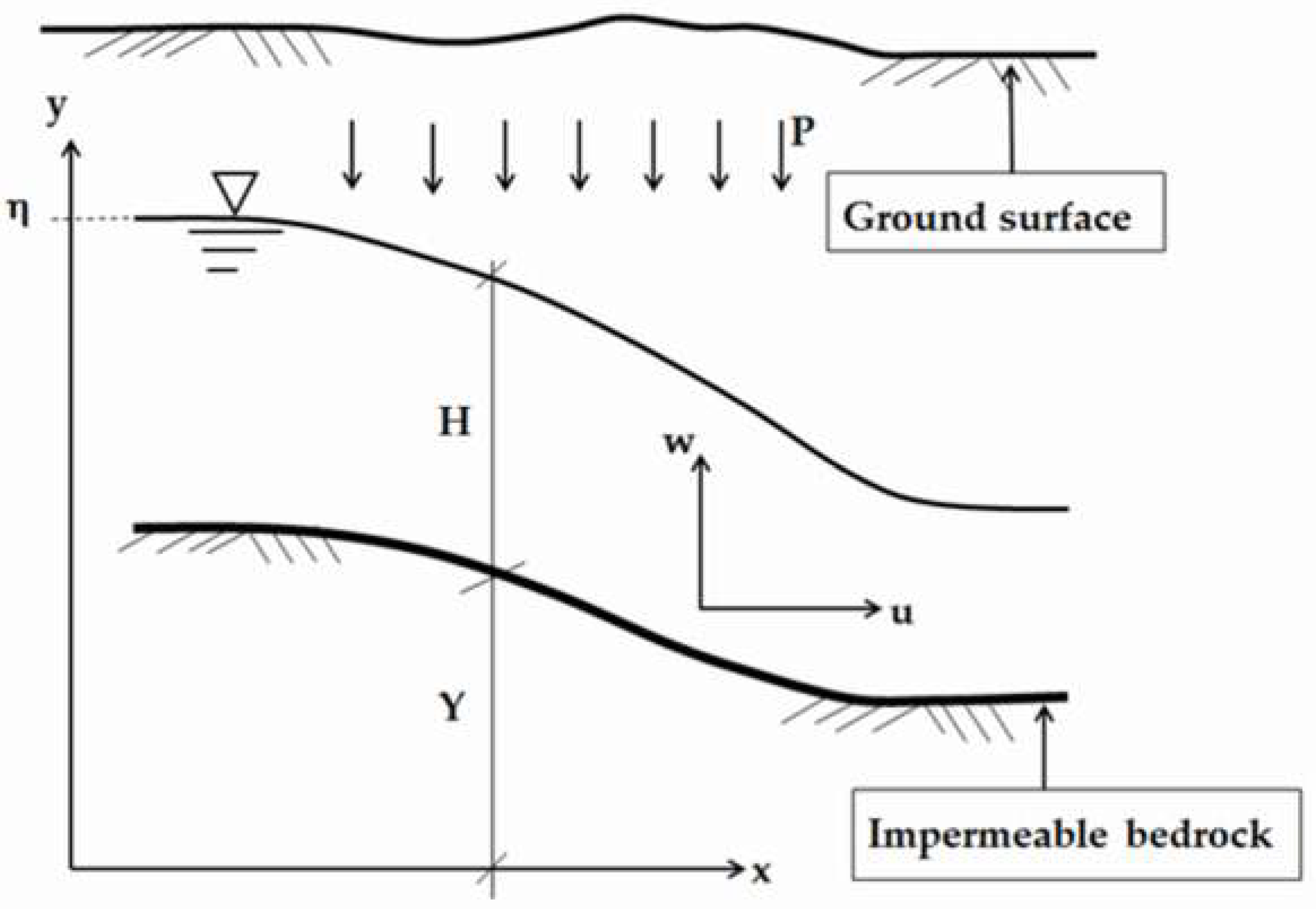
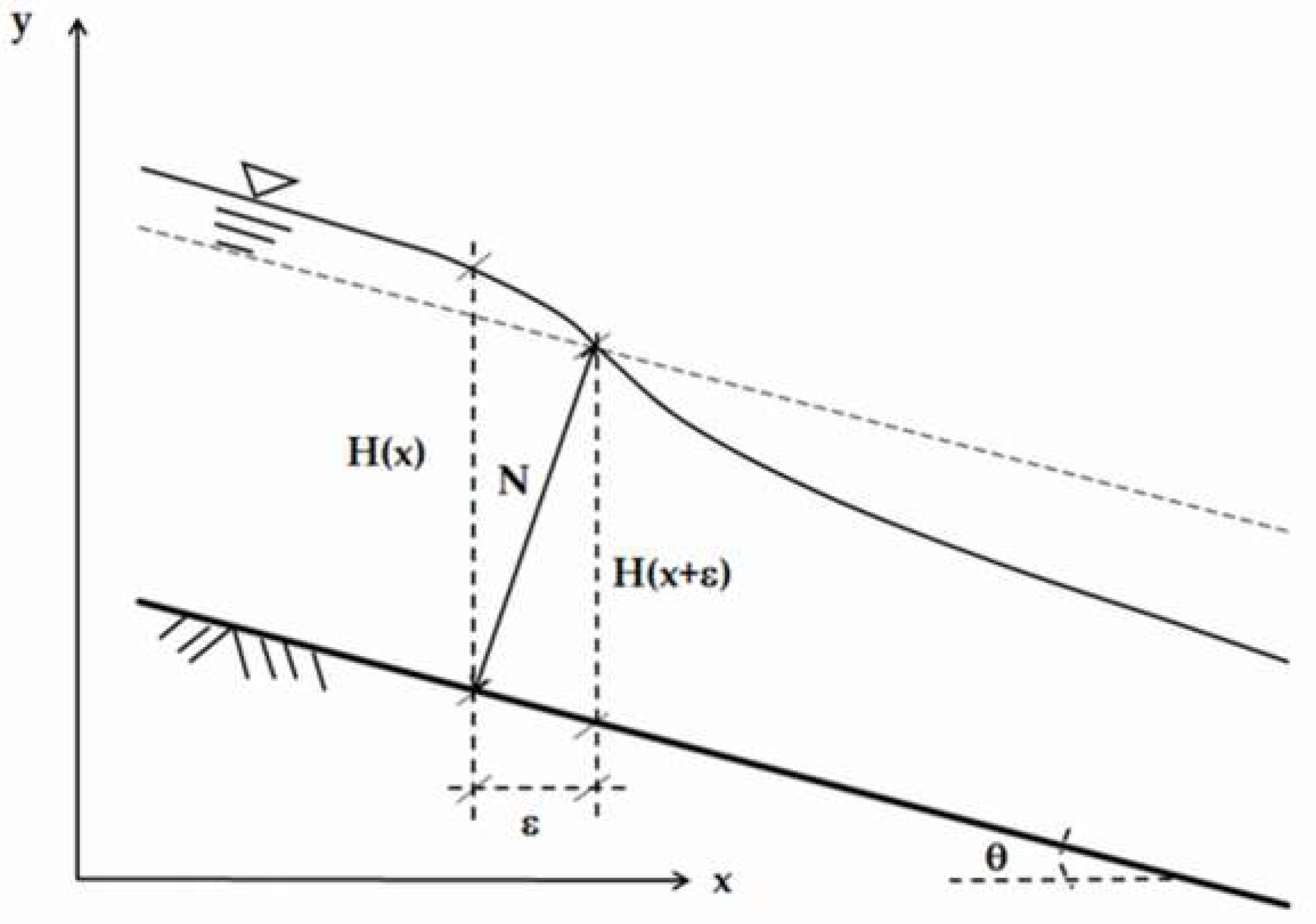
Consider a non-hydrostatic groundwater flow with a phreatic surface over steeply sloped and curved impermeable bedrock, as shown in Figure 1. A Cartesian coordinate system is chosen such that $x$ is horizontal in the streamwise direction, $y$ is vertically upward, and $z$ is horizontal in the transverse direction. For simplicity, a homogeneous and isotropic aquifer is considered here. The governing equations are derived based on a stepwise iterative approach where the first approximation corresponds to the lowest-order equation of motion for unconfined groundwater flow in a sloping aquifer. For such a gradually-varied flow situation, the expression for the piezometric or hydraulic head can be written as

$$H_p=\frac{\left(\eta -y\right)}{{\omega }_1}+\frac{\left(y-Y\right)}{{\omega }_1}+Y,$$

(2)

where $\eta$ refers to the phreatic-surface elevation; $y$ is the elevation of a point in the flow field; $Y$ is the bedrock elevation; $H_p\left(=y+p/\gamma \right)$ is the piezometric head; $p$ is the pressure; $\gamma$ is the unit weight of the fluid; and ${\omega }_1=1+{\left(Y_x\right)}^2+H_x{Y}_x$. Appendix A outlines the proof of Equation (2). Applying Darcy’s law leads to

$$u=-K\frac{\partial H_p}{\partial x}=-K\left(\frac{H_x}{{\omega }_1}+Y_x\right),$$

(3)

where $u$ is the velocity in the streamwise $x$-direction; and $H$ is the depth of flow measured vertically. In the above equation, the subscript $x$ denotes partial differentiation with respect to the horizontal axis. Subsequent approximations are applied to Equation (3) using the continuity equation and Darcy’s law, as described below. The first-order approximation for the vertical velocity component can be deduced from the integration of the 2D continuity equation as follows:

$${\displaystyle \underset{Y}{\overset{y}{\int }}\frac{\partial u}{\partial x}}dy+{\displaystyle \underset{Y}{\overset{y}{\int }}\frac{\partial w}{\partial y}}dy=\frac{\partial }{\partial x}\left({\displaystyle \underset{Y}{\overset{y}{\int }}u\left(y\right)dy}\right)+u\left(Y\right)Y_x-u\left(y\right)y_x+w-w_b=0,$$

(4)

where $w$ is the velocity in the $y$-direction.

Inserting Equation (3) into Equation (4) and applying the kinematic boundary condition at the bottom boundary, $w_b=Y_x{u}_b$, results for the vertical velocity distribution in

$$w=KH\left(\frac{H_{xx}}{{\omega }_1}+Y_{xx}\right)\xi -K{Y}_x\left(\frac{H_x}{{\omega }_1}+Y_x\right),$$

(5)

$$\xi =\frac{y-Y}{\eta -Y},$$

(6)

where $u_b$ and $w_b$ are the horizontal and vertical velocity components, respectively, at the bottom boundary; and $\xi$ is a non-dimensional vertical coordinate.

A higher-order approximation for the vertical profile of the piezometric head is deduced from the Darcy equation for the vertical velocity as

$$K{H}_p={\displaystyle \underset{y}{\overset{\eta }{\int }}w\left(y\right)\hspace{0.17em}dy}+K\left(\frac{H}{{\omega }_1}+Y\right),$$

(7)

where $\left(H/{\omega }_1+Y\right)$ is the piezometric head at the phreatic surface.

Inserting Equation (5) into Equation (7) and then integrating the resulting equation vertically yields the following higher-order expression that describes a quadratic variation of the piezometric head across a vertical section:

$$H_p=H^2\left(\frac{H_{xx}}{{\omega }_1}+Y_{xx}\right)\left(\frac{1-{\xi }^2}{2}\right)-Y_{x}H\left(\frac{H_x}{{\omega }_1}+Y_x\right)\left(1-\xi \right)+\left(\frac{H}{{\omega }_1}+Y\right).$$

(8)

Equation (8) implies that the deviation from the hydrostatic pressure distribution is due to the combined effects of the vertical velocity of the groundwater flow and the appreciable slopes of the phreatic surface and the bedrock. If the first and second terms on the right-hand side of this equation are neglected, then the piezometric head corresponding to a hydrostatic pressure distribution is recovered after setting ${\omega }_1=1.0$.

By making use of Equation (8) and Darcy’s law, a higher-order approximation for the distribution of the horizontal velocity is obtained as follows:

$$\begin{array}{ll}u=& -K{H}^2\left(\frac{H_{xxx}}{{\omega }_1}+Y_{xxx}\right)\left(\frac{1-{\xi }^2}{2}\right)-KH\left(\frac{H_{xx}}{{\omega }_1}+Y_{xx}\right)\left({\eta }_x-Y_x\left(1-\xi \right)\right)+K{Y}_{xx}H\left(\frac{H_x}{{\omega }_1}+Y_x\right)\left(1-\xi \right)\\ & +K{Y}_{x}H\left(\left(\frac{H_{xx}}{{\omega }_1}+Y_{xx}\right)\left(1-\xi \right)\right)-K\left(\frac{H_x}{{\omega }_1}+Y_x\right).\end{array}$$

(9)

In contrast to the DF approach, the nature of the higher-order approximations can be clearly identified in Equations (5), (8), and (9). For 2D unconfined groundwater flow in the vertical plane, the depth-averaged mass-conservation equation reads as [15]

$$\lambda \frac{\partial H}{\partial t}+\frac{\partial }{\partial x}\left({\displaystyle \underset{Y}{\overset{\eta }{\int }}u}dy\right)=\lambda \frac{\partial H}{\partial t}+\frac{\partial q}{\partial x}=P,$$

(10)

where $\lambda$ is the effective porosity of the aquifer; $t$ is the time; and $P$ is the rate of vertical recharge.

The variation of the phreatic-surface elevation for a non-hydrostatic groundwater-flow problem can be described by combining the above depth-averaged continuity equation with Equation (9), i.e.,

$$\begin{array}{ll}\frac{\lambda }{K}\frac{\partial H}{\partial t}=& \frac{\partial }{\partial x}\left(\frac{H}{{\omega }_1}{H}_x+\frac{H^2{H}_x}{{\omega }_1}{H}_{xx}+\frac{H^3}{3{\omega }_1}{H}_{xxx}+H{Y}_x\right)\\ & +\frac{\partial }{\partial x}\left(\left(H^2{H}_x-\frac{H^2}{2{\omega }_1}{H}_x-\frac{H^2}{2}{Y}_x\right)Y_{xx}+\frac{H^3}{3}{Y}_{xxx}\right)+\frac{P}{K}.\end{array}$$

(11)

The above equation implicitly incorporates the effects of nonuniform velocity and of non-hydrostatic pressure distributions for modelling the problems of phreatic flow accurately. For the case of 2D groundwater flow with an appreciable streamline curvature and slope over horizontal bedrock ($Y_x=Y_{xx}=Y_{xxx}=0$ and ${\omega }_1=1.0$), Equation (11) simplifies to that given by Dagan [25]. Thus,

$$\frac{\lambda }{K}\frac{\partial H}{\partial t}=\frac{\partial }{\partial x}\left(\frac{H}{{\omega }_1}{H}_x+\frac{H^2{H}_x}{{\omega }_1}{H}_{xx}+\frac{H^3}{3{\omega }_1}{H}_{xxx}\right)+\frac{P}{K}.$$

(12)

Equation (12) implies that, in contrast to the Chapman and Dressler [14] and Chapman and Ong [16] equations, the proposed model includes a higher-order correction term that takes into account the effects of the phreatic-surface and the bedrock curvatures separately. Nielsen et al. [26] investigated the applicability of this equation to oscillatory plane flow in coastal aquifers of intermediate depths. For the case of unconfined groundwater flows with negligible vertical curvature of the streamline over sloping planar bedrock, Equation (11) degenerates to a Boussinesq-type equation, structurally analogous to Childs’ [27] equation,

$$\frac{\lambda }{K}\frac{\partial H}{\partial t}=\frac{\partial }{\partial x}\left(\frac{H}{{\omega }_1}{H}_x+H{Y}_x\right)+\frac{P}{K},$$

(13)

which was adapted by Chapman [28] for analysing the phreatic-surface profile of such flows. In the case where the impermeable bedrock is horizontal ($Y_x=0$ and ${\omega }_1=1.0$), this equation becomes

$$\frac{\lambda }{K}\frac{\partial H}{\partial t}=\frac{\partial }{\partial x}\left(H{H}_x\right)+\frac{P}{K}.$$

(14)

Equation (14) corresponds to the one-dimensional DF equation for hydrostatic flows. The above analysis reveals that the proposed model is different from earlier models and incorporates a correction factor for the effects of the vertical component of the gravity-flow system. Consequently, it is a one-dimensional non-hydrostatic model for analysing the salient features of the curvilinear groundwater-flow problems. The nonlinearity of the model equations imposes difficulty to obtain a closed-form solution unless a simplifying or linearising method is applied. A numerical approach, based on the finite-difference approximation of the derivative terms, is employed here to solve the equation. This approach has been successfully applied to non-hydrostatic open-channel flow problems with the implementation of the Newton–Raphson iteration method [29,30] and of the standard optimisation method [31] as efficient solvers. Using such a numerical solution technique, the applicability of the proposed model will be systematically examined for the test cases of 2D groundwater flow with a phreatic surface, where the effect of the vertical velocity plays a significant role.

3. Seepage Flows with a Phreatic Surface

For steady accretion-free flow in an earth-fill dam resting on horizontal impermeable bedrock, Equation (11) may be written in the form

$$\frac{\partial }{\partial x}\left(\frac{\partial }{\partial x}\left(\frac{H^2}{2{\omega }_1}+\frac{H^3}{3{\omega }_1}{H}_{xx}\right)\right)=0.$$

(15)

Using Equation (8) and a little manipulation based on the relationship between discharge and velocity, the following result is obtained as in Fenton [15]:

$$\frac{\partial }{\partial x}\left({\displaystyle \underset{Y}{\overset{\eta }{\int }}{H}_p}(y)dy\right)+H_p\left(Y\right)Y_x-H_p\left(\eta \right){\eta }_x=\frac{\partial }{\partial x}\left(\frac{H^2}{2{\omega }_1}+\frac{H^3}{3{\omega }_1}{H}_{xx}\right)=-\frac{q}{K},$$

(16)

where $H_p\left(y\right)$ is the value of the piezometric head at a height $y$ above the datum. Combining Equations (15) and (16) and integrating the resulting expression twice with respect to $x$ gives

$$\frac{H^3}{3{\omega }_1}{H}_{xx}+\frac{H^2}{2{\omega }_1}=-\frac{q}{K}x+{\omega }_3,$$

(17)

where ${\omega }_3$ is an integration constant and can be determined from the known flow depth, which is specified as a boundary condition at the inflow section ($j=0$), as follows:

$${\omega }_3=\frac{H_0^3}{3{\omega }_{1,0}}{H}_{xx,0}+\frac{H_0^2}{2{\omega }_{1,0}}.$$

(18)

In the above equation, the subscript $0$ indicates that the parameters are evaluated at the inflow section. As described before, a numerical technique is the only means of attaining a solution to Equation (17) for such a steady-state potential-flow problem. Thus, the spatial derivative term in this equation is discretised by using the four-point finite-difference equation as [32] (p. 877)

$$H_{xx,j}=\frac{1}{{\left(\Delta x\right)}^2}\left(H_{j-1}-2H_j+H_{j+1}\right),$$

(19)

where $\Delta x$ is the size of the step. In order to minimise numerical error due to spatial discretisation, the size of the step was kept between 2% and 4% of the horizontal length of the model domain. The application of the discretised equation at the downstream end introduces unknown nodal values external to the computational domain. This problem is avoided by using three-point backward finite-difference approximation to the derivative term at this node. The resulting implicit set of nonlinear algebraic equations is linearised using the Newton–Raphson method with a numerical Jacobian matrix and then solved by the lower-upper (LU) decomposition method. The convergence of the numerical solutions is assessed based on the relative change in solution criterion with a convergence tolerance of ${10}^{-6}$. In the following sections, the numerical scheme will be applied to analyse the flow pattern of a gravity-flow system in rectangular and trapezoidal dams. This will include the determination of the location of the phreatic surface, the height of the discharge face, and the rate of seepage flow.

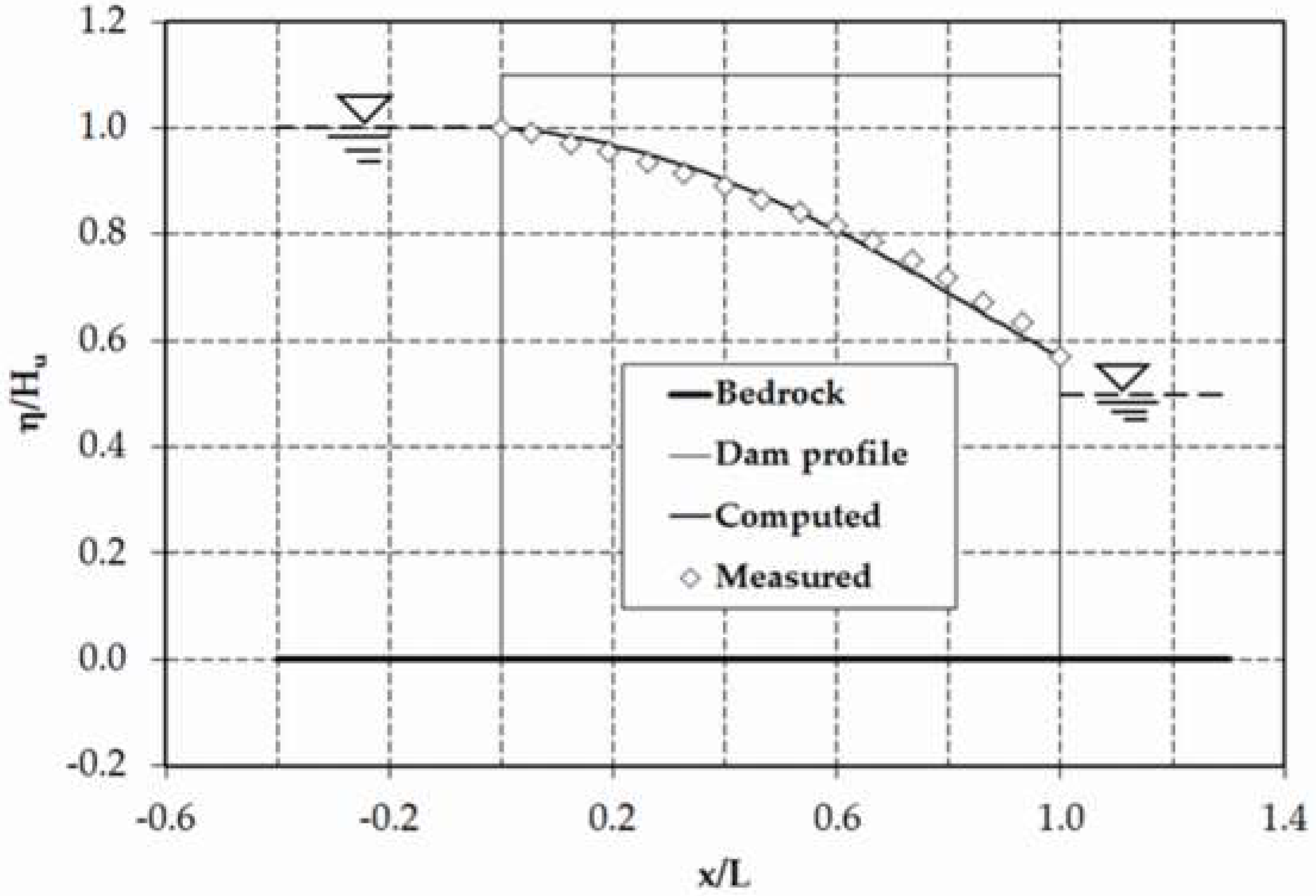
3.1. Rectangular Profile Dam

Figure 2 illustrates the steady-state seepage-flow problem involving a rectangular profile dam having an impervious foundation and different free-surface levels across its width. Since the upstream and downstream faces of the dam are subjected to hydrostatic pressure, the boundary conditions for the problem are: (i) $H=H_u$ and $H_x=0$ at $j=0$; and (ii) $H=H_d$ at $j=m$. For this unconfined flow problem, the phreatic-surface position is the only unknown and must be determined iteratively from its initial position by using a numerical solution method. Initially, it is assumed that the phreatic surface is horizontal throughout the computational domain with a height equal to the flow depth at the inflow section ($\eta /H_u=1$).

Using Darcy’s law, the general expression for the rate of seepage flow across an earth-fill dam can be obtained as follows:

$$q={\displaystyle \underset{Y}{\overset{\eta }{\int }}u\left(y\right)\hspace{0.17em}dy}=-K{\displaystyle \underset{Y}{\overset{\eta }{\int }}\frac{\partial H_p}{\partial x}dy=-K\frac{\partial }{\partial x}\left({\displaystyle \underset{Y}{\overset{\eta }{\int }}{H}_p\left(y\right)}\hspace{0.17em}dy-\frac{H^2}{2{\omega }_1}\right)}.$$

(20)

For a rectangular profile dam, integration of Equation (20) with respect to $x$ between the vertical upstream and downstream end faces yields the following equation after applying the boundary conditions at $j=0$ and $j=m$:

$$q=K\left(\frac{H_u^2-H_d^2}{2L}\right),$$

(21)

where $H_u$ and $H_d$ are the headwater and tailwater depths, respectively; $h_s$ is the height of the seepage surface; and $L$ is the bottom width of the dam in the streamwise direction or the horizontal length of the aquifer. The DF theory also gives a result similar to Equation (21). It was shown by Charnyi [33] that the value of the seepage flux given by the result of this theory is exact [34] (p. 281). For the prescribed boundary conditions at the inflow section, this equation and Equation (17) are numerically coupled to simulate the profile of the phreatic surface. In this study, all computational results are presented graphically and are expressed in non-dimensional forms such as $x/L$ or $x/H_u$, $\eta /L$ or $\eta /H_u$, and $H_p/H$.

The experimental data, consisting of phreatic-surface elevation and seepage surface height for this test problem, were obtained from Billstein [35]. The experiments were performed using the Hele-Shaw model based on the analogy between a viscous flow and flow through a porous media. He constructed a vertical model made of two parallel transparent plates with a horizontal impervious boundary at the bottom end. The plates had a length of 300 mm and an interspace width ranging from 2 mm to 16 mm. Glycerine was used as the model fluid.

The computation of the phreatic-surface elevation requires a prior knowledge of the hydraulic conductivity of the Hele-Shaw model. The magnitude of this conductivity parameter was determined by using the following equation [36] (p. 366):

$$K=\frac{b^{2}g}{12\nu },$$

(22)

where $b$ is the width of the interspace; $g$ is acceleration due to gravity; and $\nu$ is the kinematic viscosity of the fluid. Figure 3 depicts the comparison of the numerical result with experimental data for $q/K{H}_u=0.36$. It can be seen from this figure that the computed result for the phreatic-surface level showed a good correlation to the experimental data.

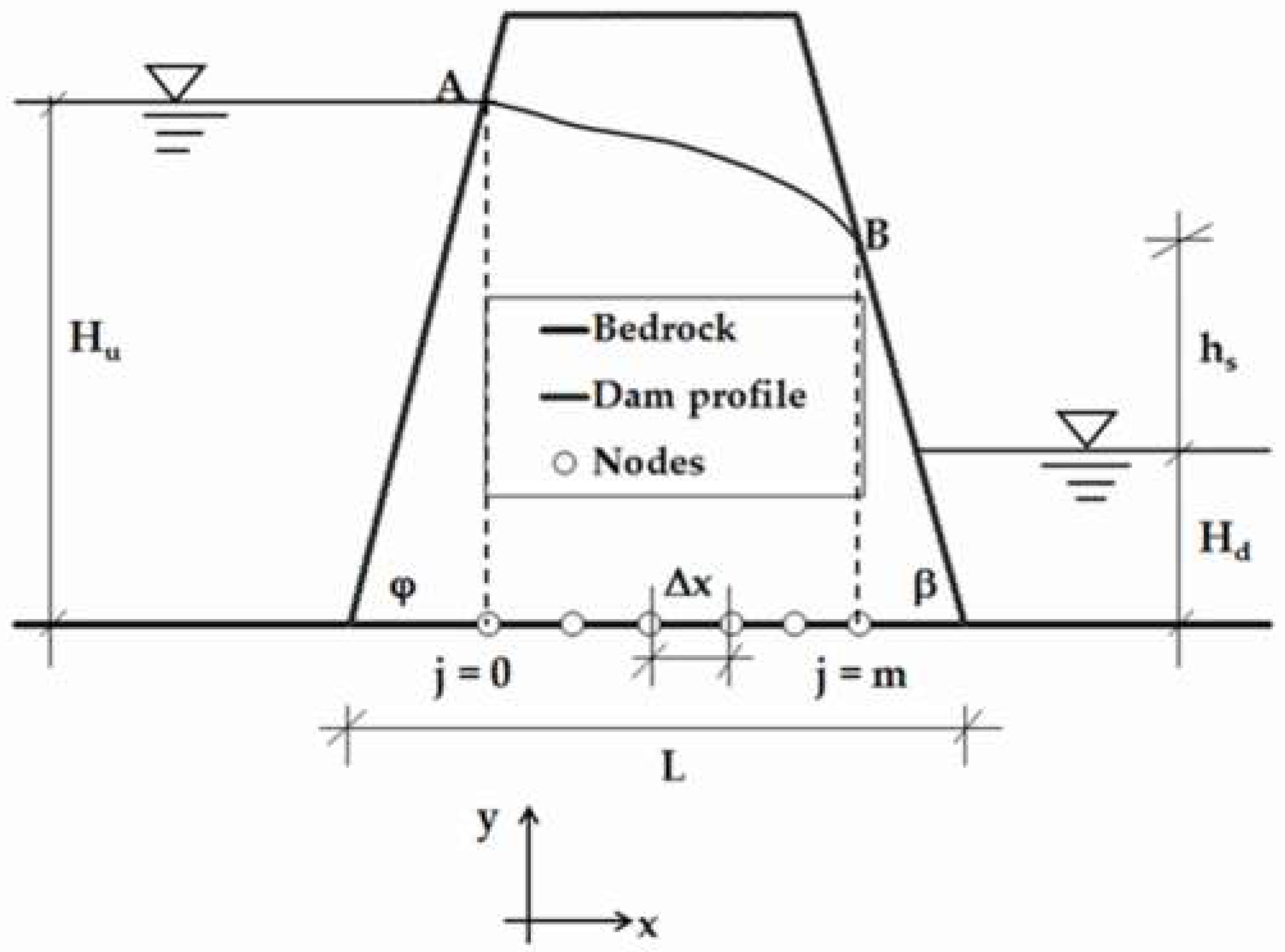
3.2. Trapezoidal Profile Dam

The preceding seepage flow analysis of the rectangular profile dam took no account of the effects of either the upstream or downstream side slope on the position of the seepage phreatic surface. In this section, seepage flow through a trapezoidal profile dam is simulated to take the side slope factor into account. For this test case, both the phreatic-surface position and the seepage discharge are unknown and are determined iteratively during the numerical computation process. As an initial guess, the height of the seepage surface is estimated by using the following approximate equation:

$$h_s=2\left(\frac{H_u^2-H_d^2}{5L}\right).$$

(23)

Figure 4 displays a typical cross-section of a homogenous trapezoidal dam resting on impervious bedrock. The phreatic surface of the dam enters the porous media at right angles to the upstream face, and it meets the surface of seepage on the downstream face, tangentially at B [37] (p. 291). This qualitative characteristic of the profile of the unconfined flow was employed here to compute the horizontal component of the surface velocities at A and B using Darcy’s law. Using the resulting expressions of equating Equation (9) to these known velocity values, Equation (20) was integrated between the vertical sections at $j=0$ and $j=m$ to give an approximate expression for the seepage flux through the trapezoidal profile dam. This equation for the horizontal seepage discharge per unit width is given by

$$q=K\left(\frac{H_u^2{\mathsf{\Gamma }}_1-{\left(H_d+h_s\right)}^2{\mathsf{\Gamma }}_2}{2(L-H_u\cot \varphi -\left(H_d+h_s\right)\cot \beta )}\right),$$

(24)

$${\mathsf{\Gamma }}_1=\left(1-\frac{2}{3}{\cos }^2\varphi \right),$$

(25)

$${\mathsf{\Gamma }}_2=\left(1-\frac{2}{3}{\sin }^2\beta \right),$$

(26)

where $\varphi$ and $\beta$ are the slopes of the upstream and downstream faces of the dam, respectively. By analysing the hydrodynamic forces within the flow region, a similar result was also presented by Kashef [38]. The above equation was directly coupled with Equation (17) to give a numerical solution for the seepage-flow problem.

At the inflow section, the slope of the phreatic surface ($H_x=-\cot \varphi$) and the flow depth were prescribed as boundary conditions. The numerical technique applied to this test case was similar to that used for the solution of seepage flow through a rectangular cross-section dam. Unlike the previous test case, the seepage discharge was determined by using Equation (24) with an iterative solution procedure based on the estimated height of the seepage surface, $h_s$. If the difference between the $h_s$ used to compute $q$ and the computed $h_s$ was significant, the iteration steps were repeated until the difference became negligible (less than 5 mm).

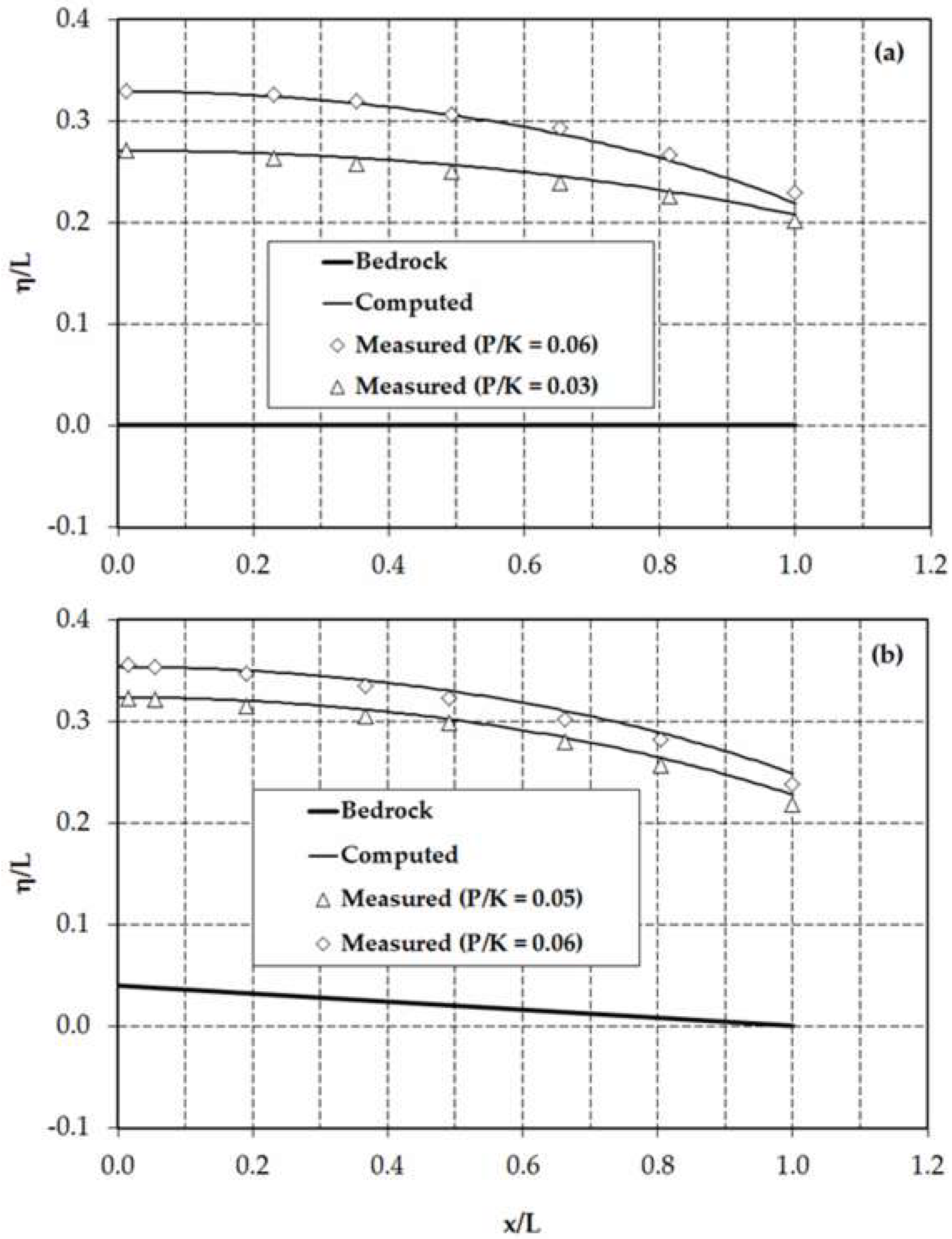
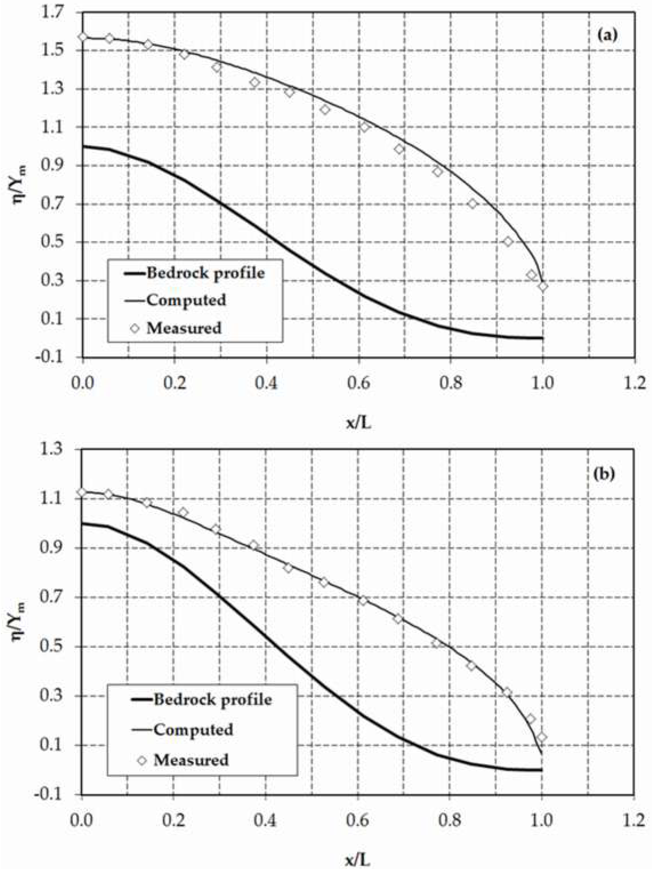
Figure 5a compares the computational result of the present method with the result of the finite-element numerical model obtained by Lacy and Prevost [39]. It is obvious from this figure that the computed result for the phreatic-surface level indicated a good agreement with the reported numerical result (mean relative error = 2.7%). The computational result was further compared in Figure 5b with the result of the electrical-model experiments [37] (p. 323), resulting in satisfactory agreement. The results for both test cases, i.e., rectangular and trapezoidal dams, revealed that the present model is capable of predicting the existence of a seepage surface on the downstream face of the dam. Nonetheless, the presence of such a surface is not recognised by the DF model [37] (p. 362). The overall qualities of the model results for both cases were satisfactory, with mean relative errors of 1.6% and 3.2% for rectangular and trapezoidal dams, respectively.

4. Recharge-Induced Curvilinear Groundwater Flows

In practice, it is common to have a phreatic-flow problem with vertical curvatures of the streamline, for instance, steady unconfined flow over a curved bedrock profile with a uniform accretion rate. For such a type of groundwater flow, Equation (11) becomes

$$\begin{array}{l}\frac{\partial }{\partial x}\left(\frac{H}{{\omega }_1}{H}_x+\frac{H^2{H}_x}{{\omega }_1}{H}_{xx}+\frac{H^3}{3{\omega }_1}{H}_{xxx}+H{Y}_x+\left(H^2{H}_x-\frac{H^2}{2{\omega }_1}{H}_x-\frac{H^2}{2}{Y}_x\right)Y_{xx}+\frac{H^3}{3}{Y}_{xxx}\right)\\ +\frac{P}{K}=0.\end{array}$$

(27)

Integrating Equation (27) with respect to $x$ and then simplifying the resulting expression using the no-flow boundary condition ($q=0$) at the hydraulic divide ($j=0$) results in a third-order nonlinear differential equation, i.e.,

$$\begin{array}{l}{H}_{xxx}+\frac{3H_x}{H}{H}_{xx}+\left(\frac{3}{H^2}+\frac{3{\omega }_1{Y}_{xx}}{H}-\frac{3Y_{xx}}{2H}\right)H_x+{\omega }_1{Y}_{xxx}-\frac{3{\omega }_1{Y}_x}{2H}{Y}_{xx}\\ +\frac{3{\omega }_1}{H^2}{Y}_x+\frac{3{\omega }_{1}P}{H^{3}K}\left(j\Delta x\right)=0.\end{array}$$

(28)

A numerical solution for the above equation was obtained by discretising the spatial derivative terms using Equation (19) and the following finite-difference approximations [32] (p. 877):

$$H_{x,j}=\frac{1}{6\Delta x}\left(-2H_{j-1}-3H_j+6H_{j+1}-H_{j+2}\right),$$

(29)

$$H_{xxx,j}=\frac{1}{{\left(\Delta x\right)}^3}\left(-H_{j-1}+3H_j-3H_{j+1}+H_{j+2}\right),$$

(30)

where $H_{x,j},\hspace{0.17em}\hspace{0.17em}{H}_{xx,j}$, and $H_{xxx,j}$ are the first, second, and third derivatives, respectively, evaluated at node $j$. For computational nodes near the downstream extreme section, these terms were estimated with the three-point backward finite differences. The discretised nonlinear equations, together with the prescribed boundary conditions at the upstream and downstream ends, were solved using the numerical method described in Section 3. Further discussion on the implementation of the boundary conditions with reference to the test problems will be presented in the following sections.

4.1. Unconfined Flow over Sloping Planar Bedrock

In this section, the feasibility of the proposed model was examined by considering a practical and challenging problem such as a recharge-induced subsurface flow over sloping planar bedrock ($Y_{xx}=Y_{xxx}=0$). For this test problem, a no-flow boundary condition at the upstream end ($H_x=-Y_x$) and atmospheric pressure at the downstream seepage surface (${\displaystyle \int p\hspace{0.17em}(y)}\hspace{0.17em}dy=0$) were imposed. Additionally, the flow depth at the upstream end ($j=0$) was specified as a boundary condition and was used to approximate the initial position of the phreatic surface. The numerical results for the profile of the phreatic surface were validated using the steady-state experimental data of Saha [40]. He performed the experiments under laminar flow conditions using a specially designed flow tank apparatus (2.5 × 60 × 115 cm) filled with uniform-size glass beads (mean diameter of 1.1 mm). An impermeable vertical wall was installed at the upstream end of the tank to mimic the drainage divide of a natural aquifer. Water was supplied from the constant head reservoir to the flow tank through a recharge generator. During the experiments, the porous media was recharged in such a way that there was no standing water in the tank. By using the Darcy column experiment, the hydraulic conductivity of the porous media was estimated ($K\cong 15$ mm/s).

Figure 6 shows the comparison of the numerical results with experimental data for the normalised phreatic-surface profiles. As can be seen from this figure, the numerical results correctly reproduced the phreatic-surface level throughout the computational domain, with a mean relative error of less than 2%. For this weakly non-hydrostatic flow over mild-slope planar bedrock, the effects of the vertical component of the flow are insignificant. As in the previous test problems, the results of the model showed the presence of seepage surface at the downstream end.

The predictions of the present model are also compared in Figure 7 with previous numerical results obtained by Youngs and Rushton [41] using the Laplace equation. The results of the present model agreed well with the 2D model results, and no appreciable differences were seen between the numerical results of the two models, except near the seepage surface at the downstream end. In this region, the maximum absolute difference did not exceed 4.5% of the horizontal length of the computational domain, $L$. For the considered ratios of rate of recharge to hydraulic conductivity, the overall performance of the current model was satisfactory for groundwater flow over planar bedrock with a moderate slope.

4.2. Unconfined Flow over Curved Bedrock

The results of the experiments conducted by Chapman and Ong [16] were selected to evaluate the performance of the model. These experiments were conducted using the Hele-Shaw viscous-flow model made of two parallel plates 13 mm thick, 127.5 cm long, and 60 cm high, separated by a gap of 1.5 mm. The bottom end of the plates was sealed by an acrylic sheet 1.5 mm thick, shaped to provide the required impermeable bedrock profile. The shape of the bedrock was designed to mimic the geometrical form of hillslope profiles. The designed bottom profile is defined by

$$\frac{Y}{Y_m}=\frac{{\alpha }_1}{Y_m}\left(\frac{{\left(L-x\right)}^{{\alpha }_2}}{{\alpha }_2{L}^{{\alpha }_2-1}}-\frac{{\left(L-x\right)}^{{\alpha }_3}}{{\alpha }_3{L}^{{\alpha }_3-1}}\right),$$

(31)

where ${\alpha }_1=3.7$; ${\alpha }_2=2.8$; ${\alpha }_3=3.3$; and $Y_m$ is the maximum height of the impermeable bedrock profile at $x=0$. The vertical recharge was simulated by the flow of glycerine from 16 hypodermic syringes connected to a manifold. The measurements of the phreatic-surface level under steady-state conditions were used to validate the numerical model results.

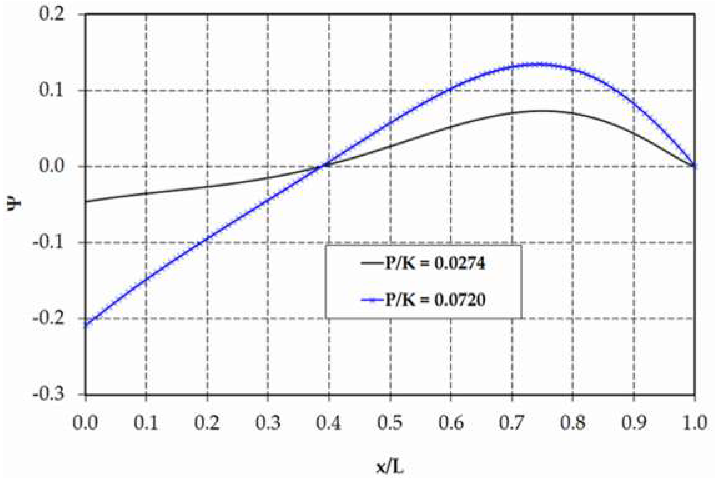
For this test problem, the profiles of the phreatic surface were simulated by specifying boundary conditions similar to the case of unconfined flow in a sloping aquifer. As shown in Figure 8, the numerical model results for the normalised phreatic-surface profile showed a good agreement with experimental data (maximum relative error less than 3%). The variation of the relative curvature of the bedrock profile, $\mathsf{\Psi }\hspace{0.17em}\left(=Y_{xx}H/{\omega }_2^{3/2},\hspace{0.17em}\hspace{0.17em}{\omega }_2=1+Y_x^2\right)$, in the streamwise horizontal direction, which was computed by using numerically simulated flow depths, is also depicted in Figure 9. It is clear from this figure that, for this moderately curved groundwater-flow problem, the effects of streamline vertical curvature are likely to be significant for the test scenario with $P/K=0.0740$. As expected, such effects play a minor role throughout the flow region, except near the outflow section ($x/L>0.8$) for the test case with a low rate of infiltration (see Figure 8b).

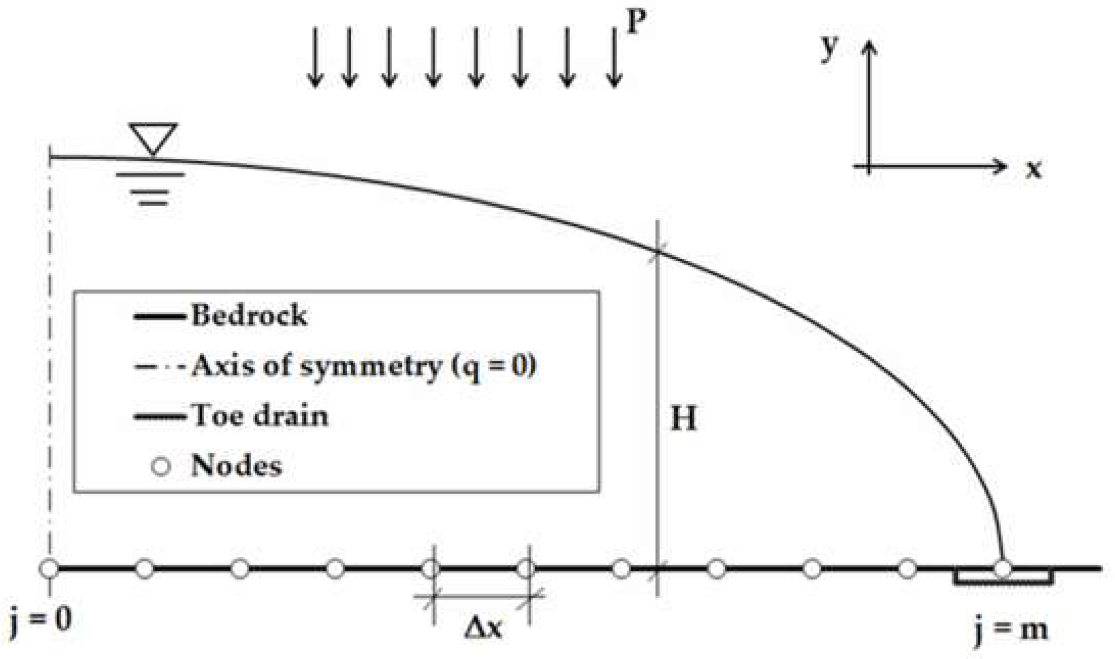
5. Unconfined Flow to Drains

Figure 10 illustrates a section of the saturated unconfined aquifer with a toe drain at the impermeable layer. For the flow problem considered here to be amenable to a 2D treatment, it is assumed that uniform flow conditions prevail along the direction parallel to the longitudinal axis of the drains. The problem is further simplified by assuming the drains to be equidistant, and steady flow conditions are reached. For this spatially-varied groundwater flow, Equation (11) may be rewritten in the form

$$\frac{\partial }{\partial x}\left(\frac{\partial }{\partial x}\left(\frac{H^2}{2{\omega }_1}+\frac{H^3}{3{\omega }_1}{H}_{xx}\right)\right)+\frac{P}{K}=0.$$

(32)

Integrating Equation (32) with respect to $x$ gives

$$\frac{\partial }{\partial x}\left(\frac{H^2}{2{\omega }_1}+\frac{H^3}{3{\omega }_1}{H}_{xx}\right)+\frac{P}{K}x={\omega }_4,$$

(33)

where ${\omega }_4$ is a constant of integration. Its value can be determined from the existing plane of symmetry at $j=0$. By imposing $q=0$ at the axis of symmetry [23] (p. 421), ${\omega }_4$ becomes

$${\omega }_4=\frac{\partial }{\partial x}\left(\frac{H^2}{2{\omega }_1}+\frac{H^3}{3{\omega }_1}{H}_{xx}\right)=-\frac{q}{K}=0.$$

(34)

Further integration of Equation (33) with respect to $x$ yields a second-order ordinary differential equation for the phreatic-surface elevation as follows:

$$\frac{H^3}{3{\omega }_1}{H}_{xx}+\frac{H^2}{2{\omega }_1}+\frac{P}{2K}{x}^2={\omega }_5,$$

(35)

where ${\omega }_5$ is a constant of integration. An expression for this constant can be found by using the boundary condition at the downstream end, $H=0$ at $j=m$, which results in

$${\omega }_5=\frac{P{L}^2}{2K}.$$

(36)

Using the numerical method described in Section 3, Equation (35) was solved numerically to simulate the recharge-induced unconfined flow to a toe drain resting on horizontal impermeable bedrock. As before, the flow depth and the phreatic-surface slope at the upstream end were specified as boundary conditions. The results of the computation were compared with the analytical solutions of Engelund [42], who employed the velocity hodograph method to analyse the problem of flow to a wide flat drain. Engelund’s solutions for the phreatic-surface elevation and the piezometric head are

$$\eta \left(x\right)={\left(\frac{P}{K}\left(L^2-x^2\right)\right)}^{1/2}+Y,$$

(37)

$$H_p^4+\frac{P}{K}\left(x^2-y^2-\left(1-\frac{P}{K}\right)L^2\right)H_p^2-{\left(\frac{P}{K}\right)}^2{x}^2{y}^2=0,$$

(38)

where $L$ is the streamwise horizontal distance from the axis of symmetry to the toe drain in which the flow depth vanishes. As pointed out by Youngs [43], the 2D solution given by Equation (37) coincides with the result of the DF approach under different simplifying assumptions. This implies that the DF approach yields accurate results for this specific plane flow problem despite the pronounced curvature of the phreatic surface in the vicinity of the toe drain.

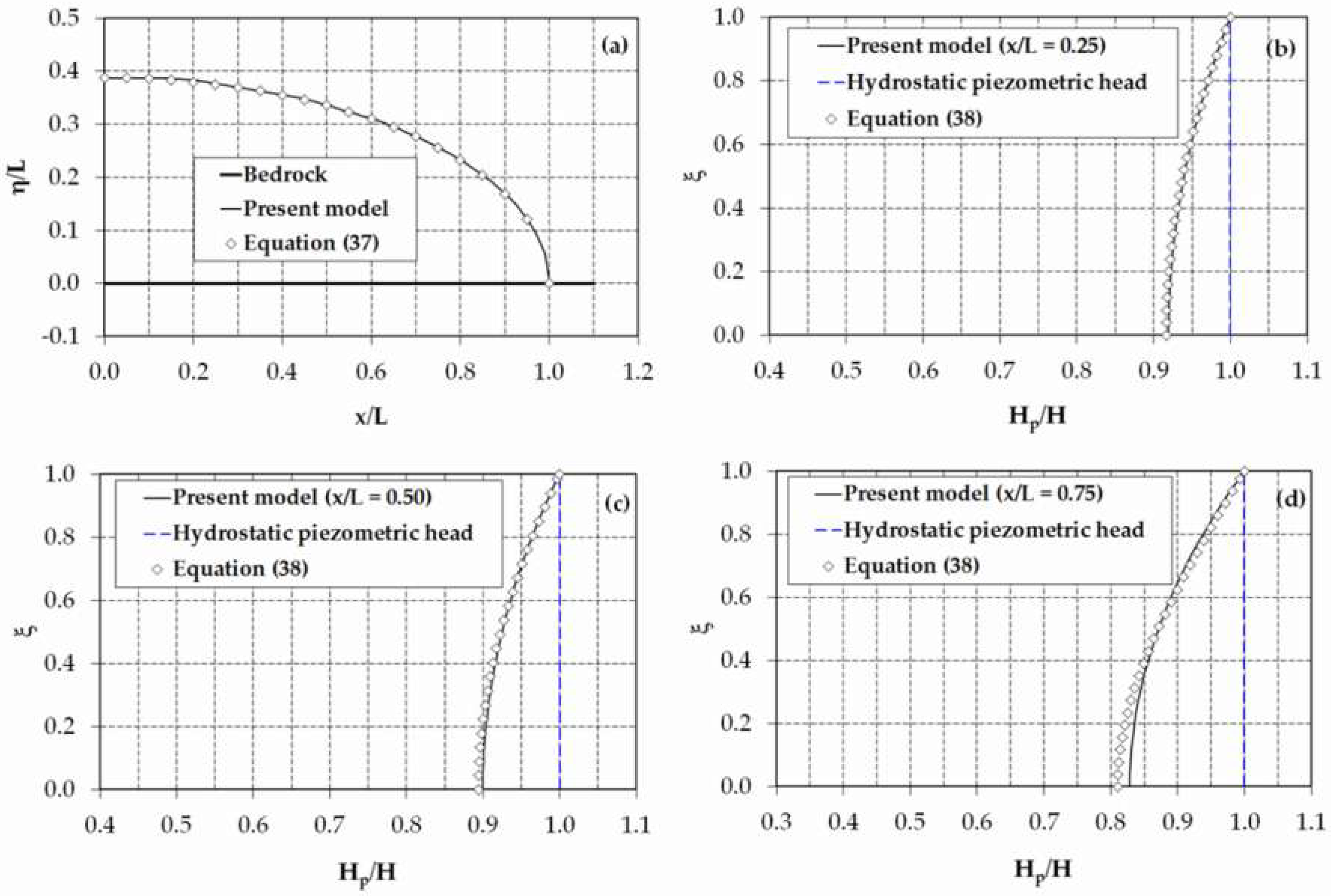
Figure 11 compares the present model results for phreatic-surface profile and piezometric head distributions at vertical sections $x/L=0.25$, $x/L=0.50$, and $x/L=0.75$ with the solutions of Equations (37) and (38), respectively, for $P/K=0.15$. For the profile of the phreatic surface, the agreement between the numerical result and the analytical solution was remarkable throughout the computational domain. As shown in Figure 11b–d, the predicted piezometric head profiles showed a good correlation with Engelund’s solutions. Nonetheless, a minor discrepancy between the numerical and analytical results can be seen from this figure near the impermeable bedrock. The differences in the piezometric head values did not exceed 2% (absolute percentage value) of the flow depth at the section. In general, the trend of the piezometric head profile was satisfactorily simulated by the proposed model. Unfortunately, the conventional DF theory, which is based on an equivalent approximation of hydrostatic pressure [44] (p. 362), overestimated the vertical distribution of the piezometric head within the flow region ($H_p/H=1.0$), as illustrated in Figure 11b–d.

6. Concluding Remarks

In this study, the classical Dupuit–Forchheimer model was extended by taking into consideration the vertical velocity of the unconfined groundwater flow. The proposed model incorporates non-hydrostatic terms that account for the effects of streamline vertical curvature and slope, and overcomes the accuracy problem of the Dupuit–Forchheimer model when simulating curvilinear groundwater flows. Thus, it differs from earlier models (e.g., [8,14,16]) in that these terms take into account the effects of the phreatic-surface and the bedrock curvatures separately. A numerical approach, based on the finite-difference approximation of the derivative terms, was employed for the solutions of the model equations. The validity of the model was demonstrated by simulating various unconfined seepage- and groundwater-flow problems with moderate curvilinear effects. The computational results for steady-state flows were compared with the results of the full two-dimensional potential-flow methods and experimental data. In order to maintain a consistent framework of comparison, the setup and discretisation of the test problems and the imposition of the boundary conditions were carefully implemented.

For the unconfined seepage-flow problems, the model accurately reproduced the profiles of the phreatic surface for flows through rectangular- and trapezoidal-profile dams. Furthermore, the seepage surface phenomenon on the downstream faces of these dams was simulated with acceptable accuracy. For the case of groundwater flow over sloping planar bedrock, the comparison results attested the capability of the model for mimicking the salient features of such types of weakly-curved unconfined flows.

Considering that a one-dimensional non-hydrostatic model was proposed to deal with complex unconfined flow processes, a good agreement between the numerical results and experimental data was attained for a recharge-induced groundwater flow over curved impermeable bedrock. This comparison result revealed the importance of the non-hydrostatic terms of the equation for modelling such a type of groundwater-flow problem. The present model overcame the limitations of the conventional Dupuit–Forchheimer approach, which is mostly applicable to groundwater flows with nearly horizontal streamlines and a mild phreatic-surface slope. Furthermore, it satisfactorily emulated the two-dimensional characteristics of the curvilinear flow field of the problem of tile drainage. Finally, the proposed numerical model could have a wide range of practical applications in connection with the stability analysis of highway and railway embankments and the design of subsurface drainage structures.