Acoustics of Bubble Arrays: Role Played by the Dipole Response of Bubbles

Abstract

A model for acoustic transmission through a 2D square crystal of R-radius bubbles with a lattice constant L was previously proposed. Assuming a purely monopole response of the bubbles, this model offers a simple analytical expression of the transmission. However, it is not applicable when the bubbles are too close to each other (L/R < 5). This article proposes an extension of the model by including the dipole response of the bubbles. Comparisons with numerical and experimental results show that the new expression gives a good estimate of the concentration at which the monopole model is no longer valid, but fails at properly predicting the transmission.

1. Introduction

As they are compressible, bubbles can easily oscillate, which makes them powerful acoustic sources and scatterers. Since the pioneering work by Minnaert [1], they have been found to be ubiquitous as sources of noise in rivers [2], the oceans [3] or even our body [4]. An interesting, and practically important, aspect of the acoustics of bubbles is the coupling they exhibit when several bubbles are close to each other. The acoustical modes of pairs of bubbles [5,6], lines of bubbles [7,8], clouds of bubbles [9,10] and arrays of bubbles [11] have been studied in the past decades.

The acoustic transmission through a 2D array of bubbles was found to be well captured by a simple analytical model [11], which proved to be efficient for predicting ultrasonic super-absorption [12] or nonlinear effects [13]. However, it is only applicable when bubbles are not too close to each other, presumably because it considers spherical oscillations of the bubbles, while other modes become important when the concentration of bubbles increases. In this article, we propose to explore the possibility of improving the model by taking into account the dipole response of the bubbles.

The article is organized as follows. In Section 2, we present the mechanism of the coupling at play between bubbles and recall the acoustic response function of a 2D square crystal of bubbles when only the monopole response of the bubbles is taken into account. We show how numerical simulations (Section 3) and experiments (Section 4) confirm the validity of the model when the arrays are not too concentrated, but show large deviation otherwise. Leaving technical details for Appendix B, Section 5 presents the results of an extension of the model, which takes dipolar terms into account.

2. A Model for the Acoustic Transmission through an Array of Bubbles

When a bubble is excited by a monochromatic pressure $Pexp[-i\omega t]$, if its radius is small compared to the wavelength of the incident wave, the pressure field it generates takes the simple form of a spherical wave with a complex amplitude p at distance r given by:

$$p(r,t)=\frac{f_s}{r}Pexp\left[i\omega (r/v-t)\right],$$

(1)

where v is the speed of sound in the host fluid and $f_s$ is the scattering function of the bubble. This function depends on the frequency of the excitation ($\omega$) and the radius of the bubble (R). It can be written as the response function of a damped harmonic oscillator:

$$f_s(\omega ,R)=\frac{R}{{\left(\frac{{\omega }_0}{\omega }\right)}^2-1-i(kR+\delta )},$$

(2)

where ${\omega }_0$ is the resonance angular frequency and $\delta$ the dissipation damping factor [14,15], $kR$ being associated with the radiative damping ($k=\omega /v$ is the acoustic wavenumber in the fluid). The resonance frequency of a bubble, known as the Minnaert resonance [1], is remarkable because of its low-frequency character: for a $0.1$ mm-radius air bubble in water, for example, ${\omega }_0/2\pi =32$ kHz, which corresponds to an acoustic wavelength in water of about $47$ cm, hence a factor of almost 500 between the radius of the resonant scatterer and the exciting wavelength.

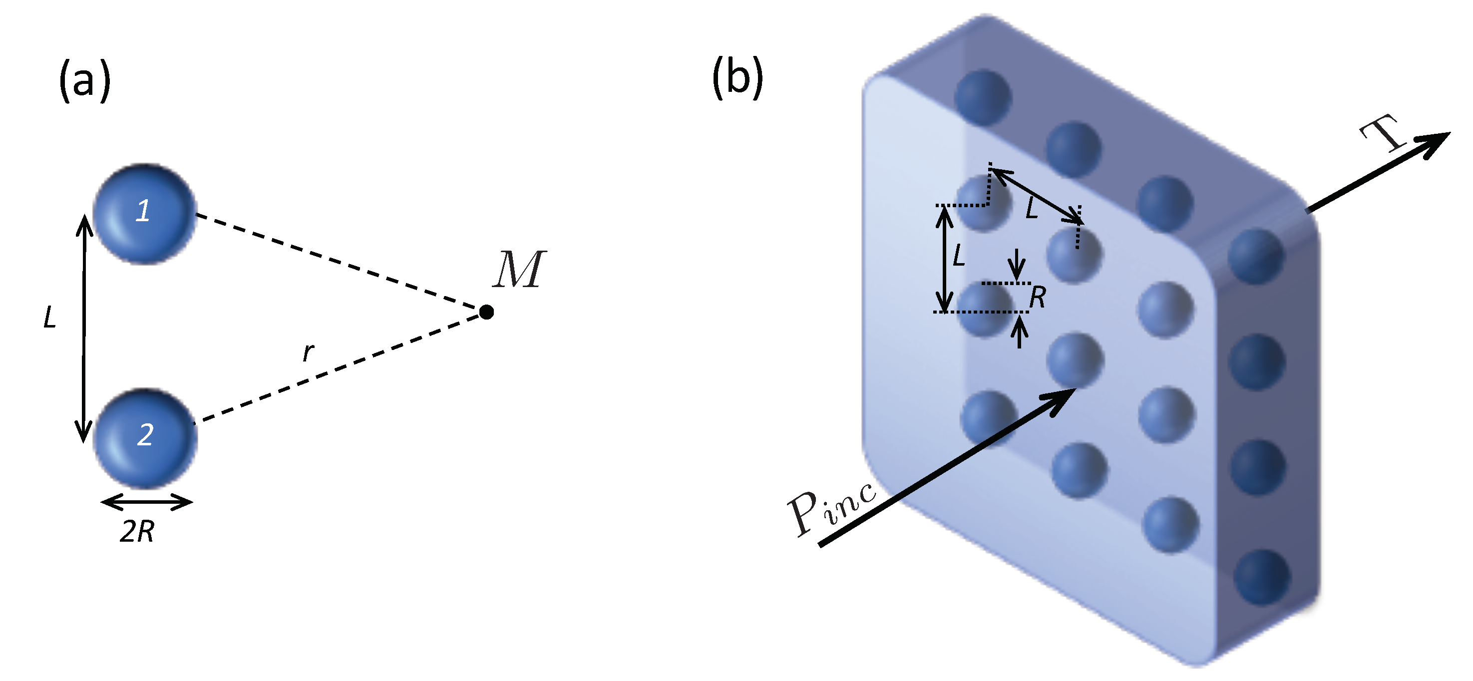
An interesting effect, due to the intense acoustic field the scatter, is the strong acoustic coupling that takes place between several bubbles. As an illustration, let us look at the case of two identical bubbles separated by a distance L and excited by the same incident pressure $p_{\mathrm{inc}}$, at angular frequency $\omega$ (see Figure 1a). The total pressure experienced by Bubble 1, $p_1$, is the sum of the incident field and the pressure scattered by Bubble 2:

$$p_1=p_{\mathrm{inc}}+p_2\frac{f_s}{L}exp\left[ikL\right],$$

(3a)

where $p_2$ is the total pressure experienced by Bubble 2, which has the symmetrical form:

$$p_2=p_{\mathrm{inc}}+p_1\frac{f_s}{L}exp\left[ikL\right].$$

(3b)

Solving Equations (3), one obtains that the total pressure for each bubble is given by:

$$p_1=p_2=p_{\mathrm{inc}}\times {\left(1-\frac{f_s}{L}exp\left[ikL\right]\right)}^{-1}.$$

(4)

Then, looking at the pressure generated by the couple of bubbles at Point M (see Figure 1a), we obtain:

$$\begin{array}{cc}\hfill p_M& =p_1\frac{f_s}{r}exp\left[ikr\right]+p_2\frac{f_s}{r}exp\left[ikr\right]\hfill \\ & =p_{\mathrm{inc}}\frac{f_s^{\left(2\right)}}{r}exp\left[ikr\right],\hfill \end{array}$$

(5)

where we used Equations (2) and (4) to express the scattering function for the couple of bubbles:

$$f_s^{\left(2\right)}=\frac{2R}{{\left(\frac{{\omega }_0}{\omega }\right)}^2-1-\frac{R}{L}coskL-i(kR+\frac{R}{L}sinkL+\delta )}.$$

(6)

It thus appears that the maximum response of the couple of bubbles is not for $\omega ={\omega }_0$, as in the case of an individual bubble, but for $\omega ={\omega }_0/\sqrt{1+(R/L)cos\left(kL\right)}$. The effect is stronger if the bubbles are close to each other ($kL\ll 1$), and it leads to a decrease of the resonant frequency. Note that, in this case, the radiative damping is doubled; a phenomenon known as super-radiation [16].

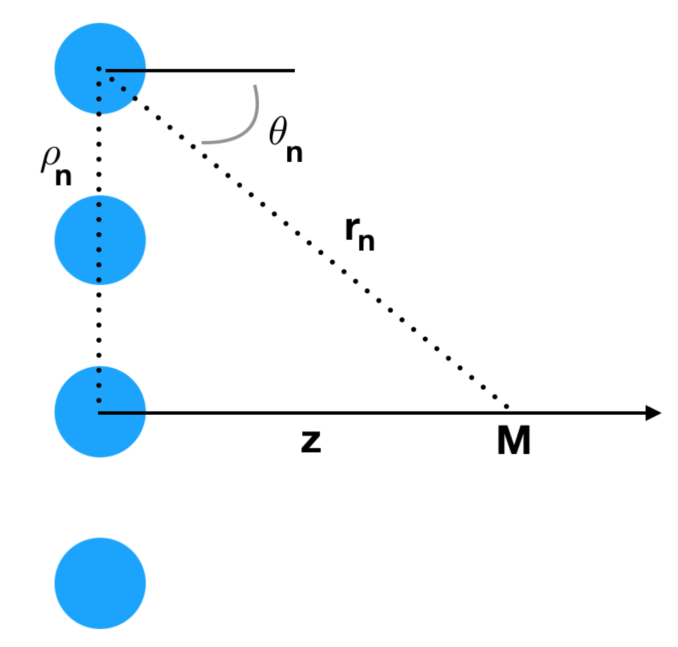
The previous approach can be extended to the case of an infinite 2D array of identical bubbles in the x,y plane (see Figure 1b). When all the bubbles are excited by $p_{\mathrm{inc}}$, the total pressure field they generate takes the form of two plane-waves, in the $+z$ and $-z$ directions: $F_s{p}_{\mathrm{inc}}exp\left[ikz\right]$ and $F_s{p}_{\mathrm{inc}}exp[-ikz]$. For bubbles of radii R on a square lattice, with a lattice constant L, the response function of the array is, for $kL\ll 1$,

$$F_s\left(\omega \right)=\frac{iKR}{{({\omega }_0/\omega )}^2-I-i(KR+\delta )},$$

(7a)

with $K=2\pi /\left(k{L}^2\right)$ and $I=1-2\sqrt{\pi }R/L$ (see the details in [11]). From Equation (7a), it is straightforward to determine the transmission through a layer of bubbles for a plane wave at normal incidence:

$$T=1+F_s.$$

(7b)

The minimum of transmission is predicted to be $\delta /(KR+\delta )$ and to happen at a frequency given by:

$$\frac{{\omega }_{\min }}{{\omega }_0}=\frac{1}{\sqrt{1-2\sqrt{\pi }R/L}}.$$

(8)

The minimum of transmission is thus for a frequency higher than the Minnaert frequency. This behavior might seem contradictory with the previous example of a couple of bubbles, as well as with the general behavior of clouds of bubbles that are known to exhibit a collective resonance at a frequency lower than the Minnaert frequency of the individual bubbles [9,17]. It can be explained by the infinite size of the array and by the long-range coupling between the bubbles. Indeed, as can be seen in Equation (6), bubbles that are at a distance r such that $coskr=-1$ will contribute to an increase of the resonant frequency of the system; respectively, the bubbles in the next half-wavelength ring will contribute to a decrease of the frequency. As the number of bubbles in each ring compensates the $1/r$ range of the coupling, each ring has exactly the same contribution. One could thus expect to obtain no frequency shift. However, because there is a lack of bubbles in the first ring, close to the central bubble, the net effect is effectively an increase of the frequency.

3. Numerical Simulations

The predicted transmission of Equations (7) can be tested by numerical simulations. We performed two types of simulations: one with a Multiple Scattering Theory (MST) code (Multel) [18], the other one with a Finite Element Method (FEM) (Using COMSOL Multiphysics v. 5.2. www.comsol.com. COMSOL AB, Stockholm, Sweden). In both cases, an infinite array of air bubbles was considered, with a radius of $0.1$ mm, and several lattice constants were inspected. For FEM simulations, the viscosities of the fluids were considered, which means that viscous dissipation was taken into account. 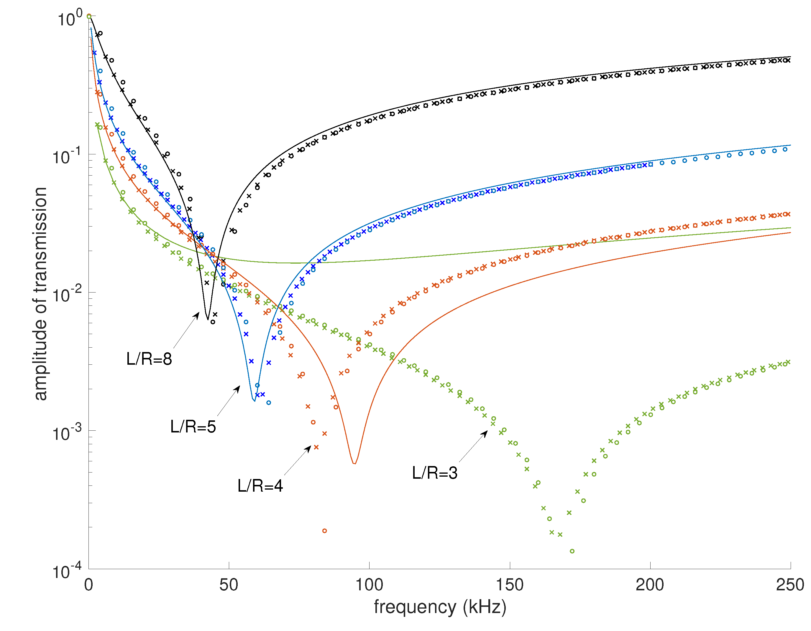For MST, however, only dissipation of the monopole mode was included, by using an ad-hoc complex velocity in air, as detailed in [11]. The results of the simulations are reported in Figure 2, in which the amplitude of transmission is shown as a function of frequency for different concentrations of bubbles: $L/R=8$, 5, 4 and 3. We see that for $L/R>5$, the model leads to a reasonable prediction of the transmission. For arrays with bubbles closer to each other, however, the agreement is not satisfactory. In the $L/R=4$ case, the model over-predicts the frequency shift. For the $L/R=3$ array, the simulations still exhibit a clear minimum, around $170$ kHz, whereas the model predicts a much flatter behavior, with a higher transmission level.

4. Experimental Results

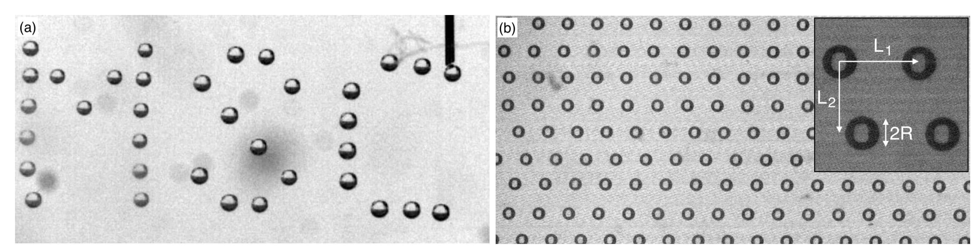
Experiments are also possible to measure the acoustic transmission through an array of bubbles. In this case, the fluid is not water, but a yield-stress fluid, which can trap bubbles and is acoustically very similar to water. We developed two techniques of injection. The first one, illustrated in Figure 3a, consists of moving a small capillary at a chosen location and then injecting a single bubble. By programming the successive positions visited by the capillary, one can thus obtain the desired pattern. This technique, however, is time consuming, which is a problem for injecting large samples. Indeed, the lifetime of a bubble is finite, because its gas tends to dissolve in the fluid. If the injection is too slow, there is therefore a risk that the first bubble has already disappeared by the time the last bubble is injected. As a consequence, we usually employ a quicker technique that consists of moving the same capillary at a constant speed along a horizontal line. If the capillary is under pressure, it delivers bubbles at regular intervals. By injecting lines at different heights, one can obtain a 2D structure as the one displayed in Figure 3b. Details on this technique can be found in [11].

Note that the samples obtained by the rapid technique are not truly 2D crystals of bubbles: if the distance between successive bubbles in a row is fairly constant, the alignment from one line to the other is not preserved. As shown in the inset of Figure 3b, we measured distance $L_1$ between neighboring bubbles in a row and distance $L_2$ from one line to the other. The lattice constant was then estimated by taking $L=\sqrt{L_1{L}_2}$, i.e., the average distance that represents the surface area concentration of bubbles.

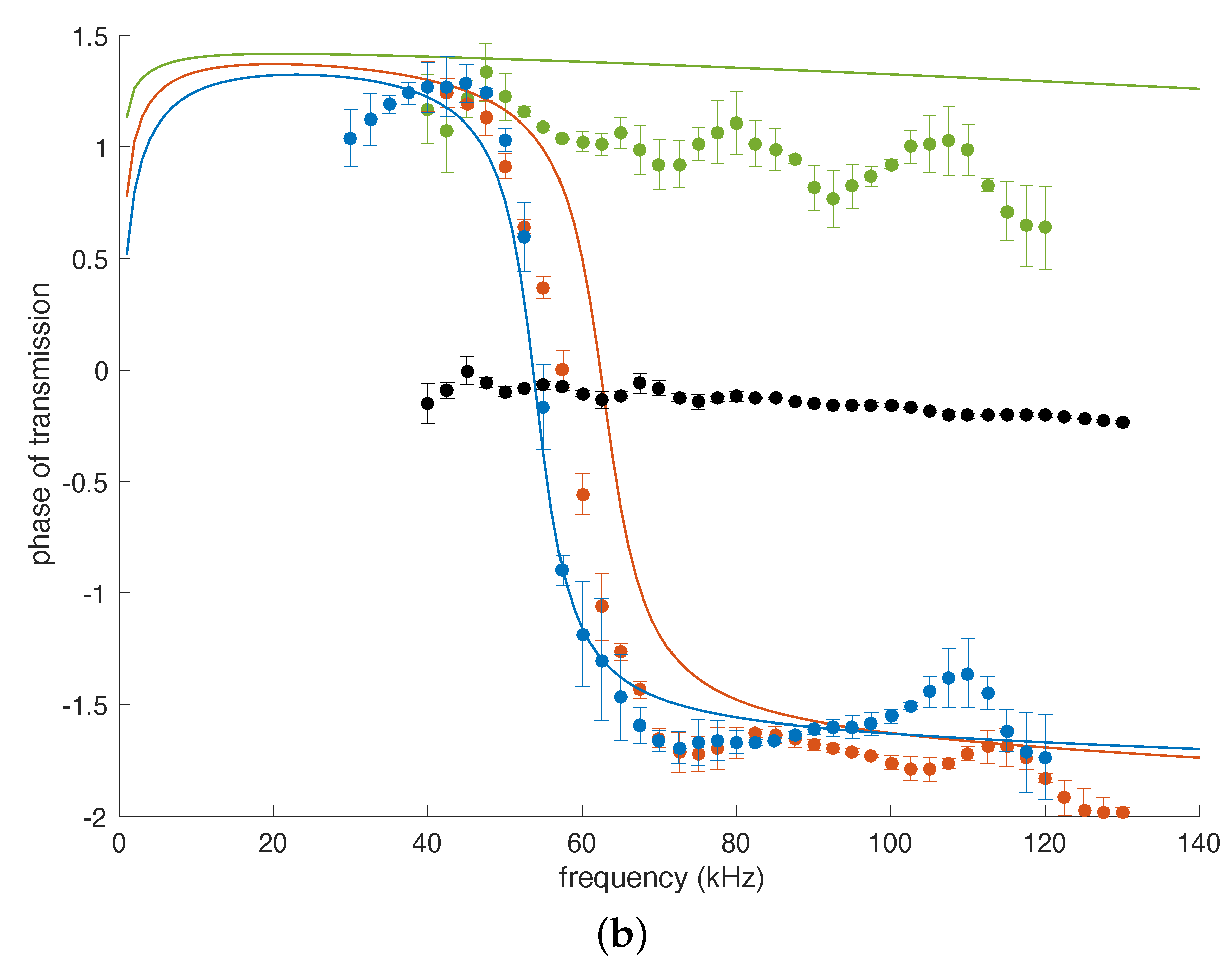
We injected arrays of bubbles in a cell filled with yield-stress fluid and placed the cell in a large tank of water, between two ultrasonic transducers. We were thus able to measure the transmission through the array of bubbles (see [11] for details on the technique). Figure 4 shows the amplitude and phase of the transmission recorded for three different arrays (see

Table 1. Geometrical parameters of the three samples of Figure 4. Sample 2 ($L/R=4.5$) is the one shown in Figure 3b.

Sample	R	${\mathit{L}}_1$	${\mathit{L}}_2$	$\mathit{L}/\mathit{R}$
1	$96 \mathsf{\mu }$m	$514 \mathsf{\mu }$m	$573 \mathsf{\mu }$m	5.7
2	$110 \mathsf{\mu }$m	$527 \mathsf{\mu }$m	$465 \mathsf{\mu }$m	4.5
3	$110 \mathsf{\mu }$m	$376 \mathsf{\mu }$m	$276 \mathsf{\mu }$m	2.9

for their characteristics), compared to the model prediction. The results are very comparable to the numerical study: the agreement is correct for $R/L=5.7$; the model predicts a too large shift in frequency for $L/R=4.5$; and for the highest concentration ($L/R=2.9$), the predicted transmission is too high compared to the measurements.

5. Discussion

The model has been shown to fail when bubbles in the array are too close to each other, typically for $L/R<5$. An idea for improvement is to remove the assumption of a purely monopolar response of the bubbles. Indeed, a spherical response is expected for a single bubble, given the large wavelength of the acoustic field at resonance, but when many bubbles are getting close to each other, one may wonder whether the responses of higher order could not be exalted. We propose to examine the role of the dipole contribution.

Let us extend Equation (1) to the case of a bubble excited by a pressure P and a pressure gradient $P^{\prime }=\mathrm{d}P/\mathrm{d}z$. The scattered field is then given by:

$$p(r,\theta )=P{f}_s\frac{{\mathrm{e}}^{ikr}}{r}-i{P}^{\prime }{f}_s^{\prime }\frac{{\mathrm{e}}^{ikr}}{kr}\left(1+\frac{i}{kr}\right)cos\theta ,$$

(9)

where $\theta$ is the angle with the z direction and $f_s^{\prime }$ the dipole scattering function of the bubbles. For the bubbles, we consider that a good approximation of this response function is $f_s^{\prime }=-k^2{R}^3$ (see Appendix A). Note that, at resonance, $f_s^{\prime }$ is four orders of magnitude less than $f_s$, which justifies our previous assumption. As detailed in Appendix B, the dipole response of the bubble array adds up with the monopole one, with a response function $F_s^{\prime }$:

$$\begin{array}{rr}\hfill T& =1+F_s+F_s^{\prime }\hfill \end{array}$$

(10)

$$\begin{array}{ll}& =1+\frac{iKR}{{({\omega }_0/\omega )}^2-I-i(KR+\delta )}-\frac{iKR{\left(kR\right)}^2}{1+2.88\pi {(R/L)}^3}.\hfill \end{array}$$

(11)

The dipole scattering of the bubbles being much weaker than the monopole one, we could expect the last term of Equation (11) to bring a negligible contribution to the transmission. This is not always true because rather than comparing $F_s^{\prime }$ to $F_s$, one needs to compare $F_s^{\prime }$ to $1+F_s$, which reaches small values close to the minimum of transmission. We can establish that monopole and dipole contributions will be of the same order of magnitude when $\delta /KR\simeq KR{\left(kR\right)}^2$, which results in the following criterion on $L/R$:

$$L/R={\left(\frac{\delta }{4{\pi }^2}\right)}^{-1/4}.$$

(12)

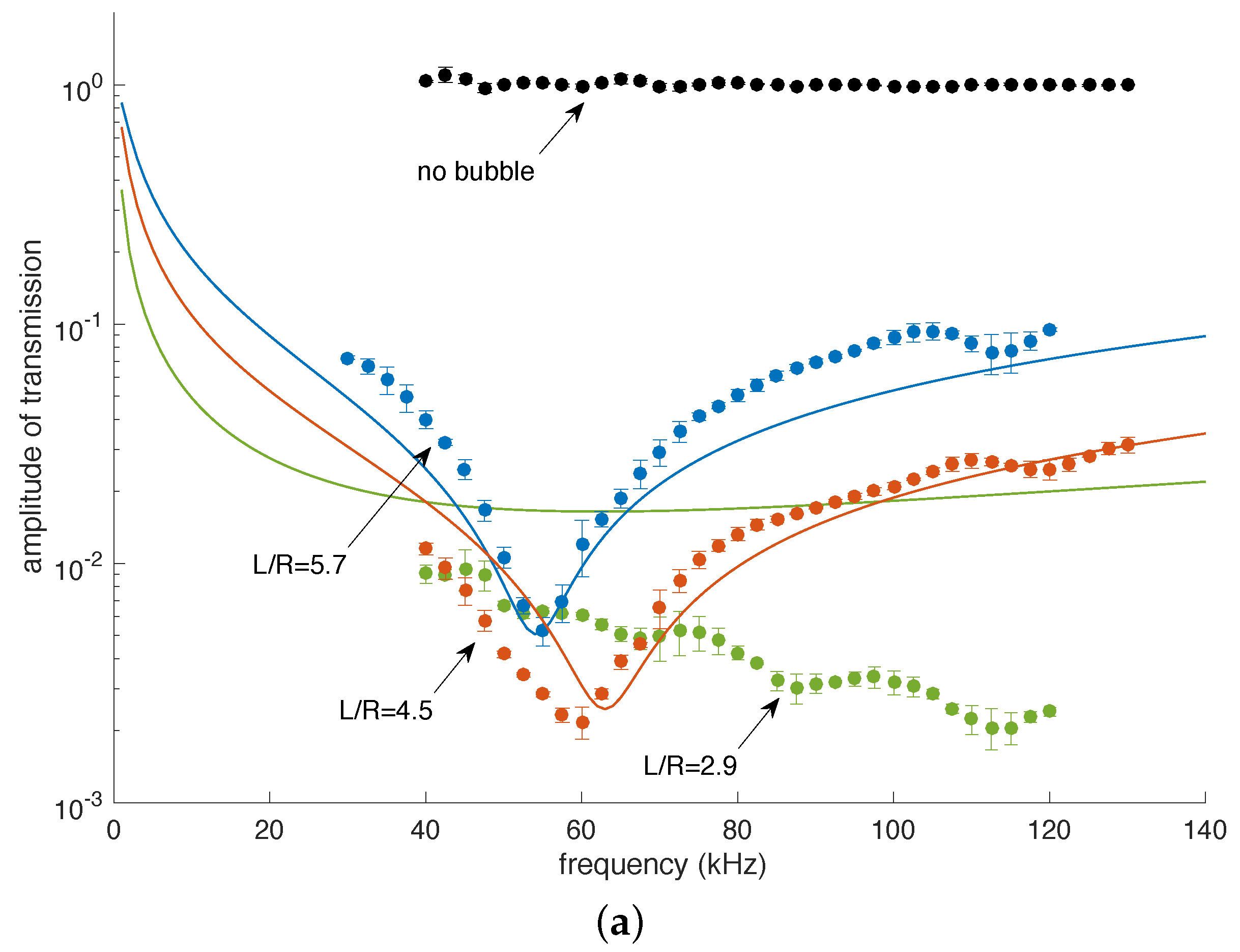
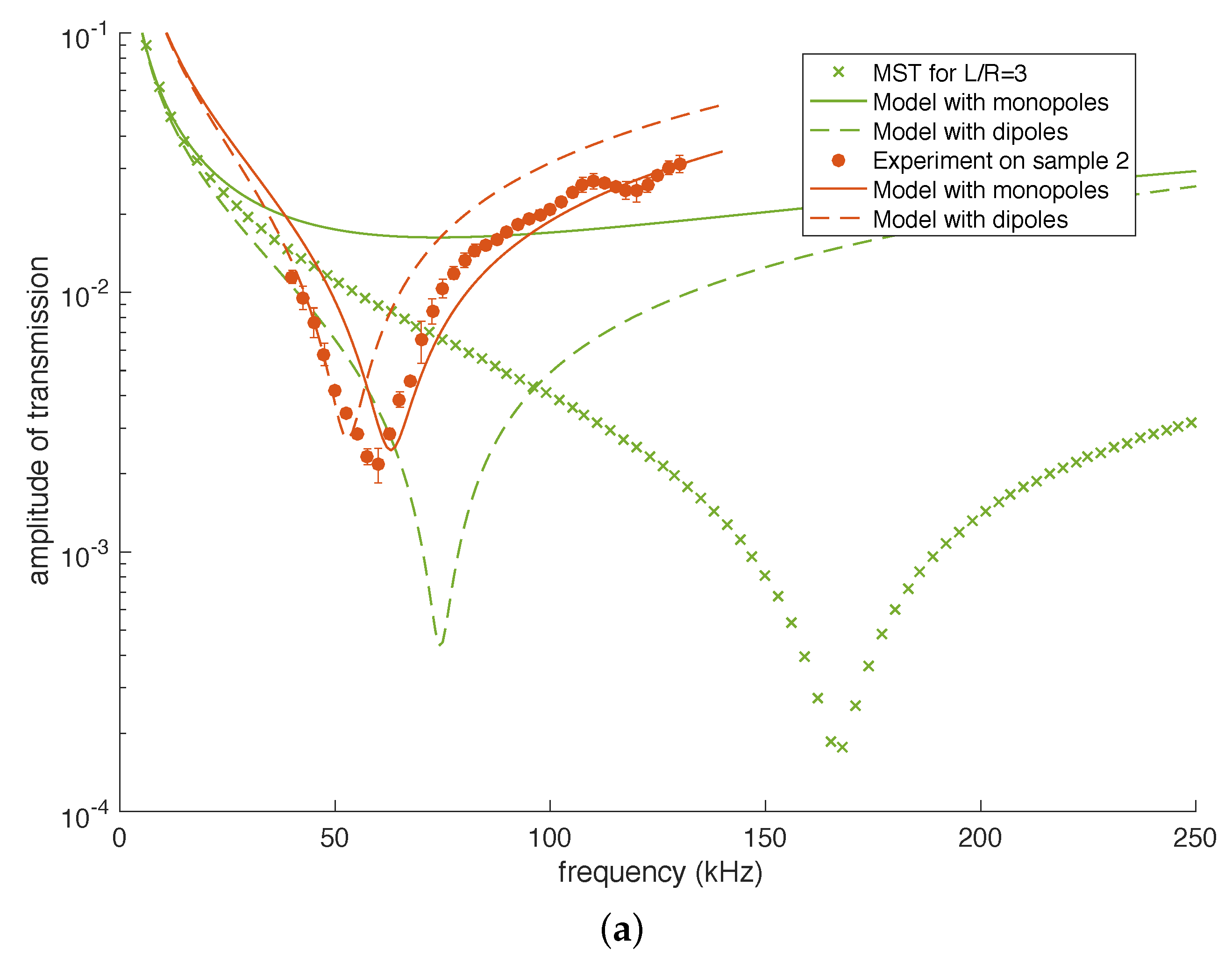
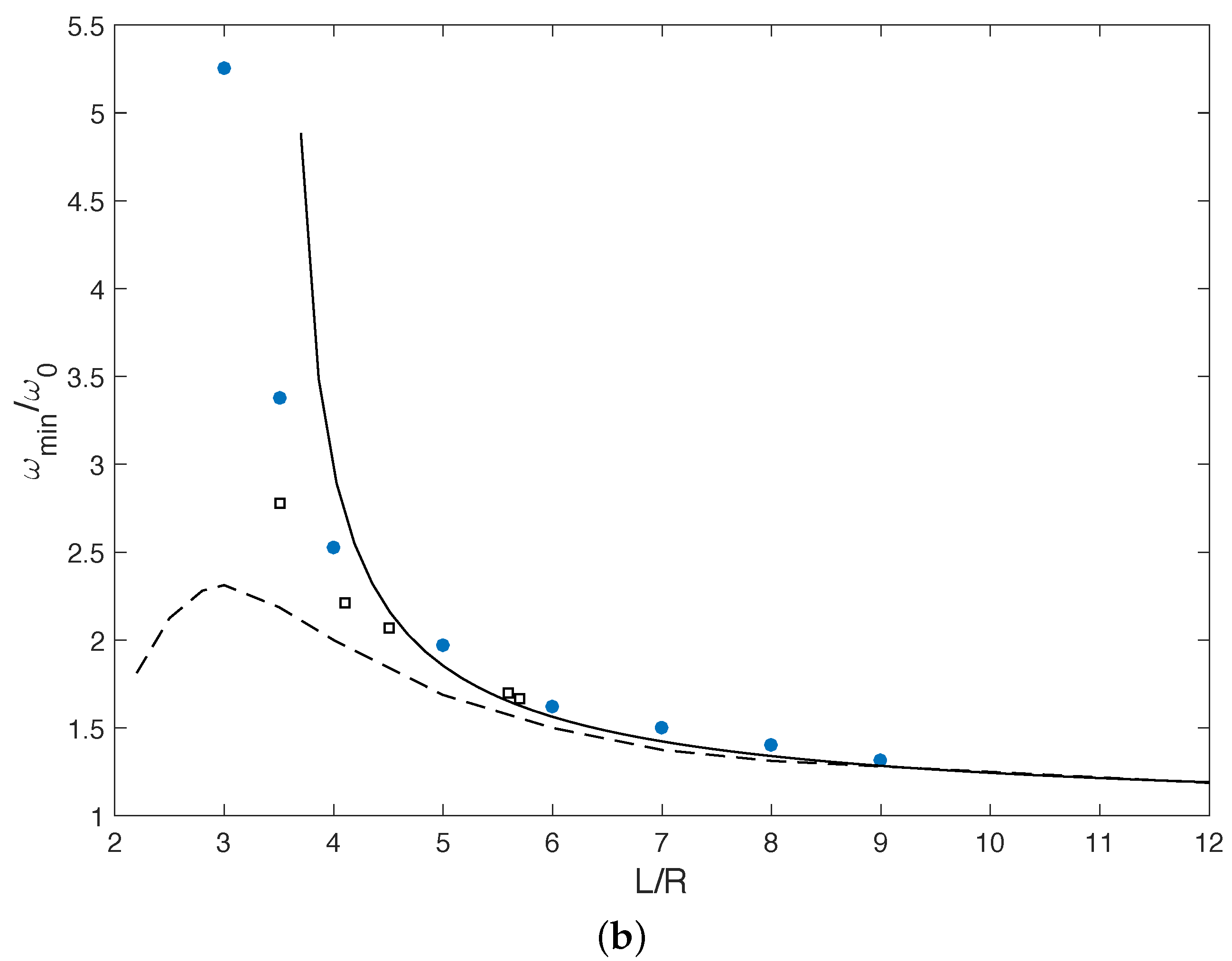
In our case of $0.1$-mm bubbles in water or yield-stress fluid, we have $\delta \simeq 0.1$, giving a criterion of $L/R\simeq 4.5$. This is indeed compatible with our observation that the monopole model is sufficient as long as $L/R>5$. However, the correction brought by this dipole model does not give a satisfactory comparison with the simulations and the experiments, as illustrated in Figure 5a for two cases. The minimum of transmission is well shifted to lower frequency, as required, but the shift is too large. In Figure 5b, we report the frequency of the minimum of transmission as a function of $L/R$, as found in the simulations and the experiments, and as predicted by the two models. It is clear that the dipole model does not bring any improvement to the theory. It probably means that other modes of deformation of the bubbles must be taken into account if one wants to properly model the transmission for arrays with $L/R<5$. In such a case, a simple analytical expression will not be available, which means that numerical simulation remains the best tool for studying such concentrated configurations.

References

1. Minnaert, M. On musical air-bubbles and the sounds of running water. Lond. Edinb. Dublin Philos. Mag. J. Sci. 1933, 16, 235–248. [Google Scholar] [CrossRef]
2. Leighton, T.G.; Walton, A.J. An experimental study of the sound emitted from gas bubbles in a liquid. Eur. J. Phys. 1987, 8, 98. [Google Scholar] [CrossRef]
3. Prosperetti, A. Bubble-related ambient noise in the ocean. J. Acoust. Soc. Am. 1988, 84, 1042–1054. [Google Scholar] [CrossRef]
4. Chandran Suja, V.; Barakat, A.I. A Mathematical Model for the Sounds Produced by Knuckle Cracking. Sci. Rep. 2018, 8, 4600. [Google Scholar] [CrossRef] [PubMed]
5. Strasberg, M. The pulsation frequency of nonspherical gas bubbles in liquids. J. Acoust. Soc. Am. 1953, 25, 536–537. [Google Scholar] [CrossRef]
6. Hsiao, P.Y.; Devaud, M.; Bacri, J.C. Acoustic coupling between two air bubbles in water. Eur. Phys. J. E 2001, 4, 5–10. [Google Scholar] [CrossRef] [Green Version]
7. Tolstoy, I.; Tolstoy, A. Line and plane arrays of resonant monopole scatterers. J. Acoust. Soc. Am. 1990, 87, 1038–1043. [Google Scholar] [CrossRef]
8. Manasseh, R.; Nikolovska, A.; Ooi, A.; Yoshida, S. Anisotropy in the sound field generated by a bubble chain. J. Sound Vib. 2004, 278, 807–823. [Google Scholar] [CrossRef]
9. Yoon, S.; Crum, L.; Prosperetti, A.; Lu, N. An investigation of the collective oscillations of a bubble cloud. J. Acoust. Soc. Am. 1991, 89, 700–706. [Google Scholar] [CrossRef]
10. Roy, R.A.; Carey, W.; Nicholas, M.; Schindall, J.; Crum, L.A. Low-frequency scattering from submerged bubble clouds. J. Acoust. Soc. Am. 1992, 92, 2993–2996. [Google Scholar] [CrossRef]
11. Leroy, V.; Strybulevych, A.; Scanlon, M.; Page, J. Transmission of ultrasound through a single layer of bubbles. Eur. Phys. J. E 2009, 29, 123–130. [Google Scholar] [CrossRef] [PubMed]
12. Leroy, V.; Strybulevych, A.; Lanoy, M.; Lemoult, F.; Tourin, A.; Page, J.H. Superabsorption of acoustic waves with bubble metascreens. Phys. Rev. B 2015, 91, 020301. [Google Scholar] [CrossRef]
13. Lombard, O.; Barrière, C.; Leroy, V. Nonlinear multiple scattering of acoustic waves by a layer of bubbles. EPL (Europhys. Lett.) 2015, 112, 24002. [Google Scholar] [CrossRef]
14. Devin, C., Jr. Survey of thermal, radiation, and viscous damping of pulsating air bubbles in water. J. Acoust. Soc. Am. 1959, 31, 1654–1667. [Google Scholar] [CrossRef]
15. Prosperetti, A. Thermal effects and damping mechanisms in the forced radial oscillations of gas bubbles in liquids. J. Acoust. Soc. Am. 1977, 61, 17–27. [Google Scholar] [CrossRef]
16. Feuillade, C. Scattering from collective modes of air bubbles in water and the physical mechanism of superresonances. J. Acoust. Soc. Am. 1995, 98, 1178–1190. [Google Scholar] [CrossRef]
17. Leroy, V.; Devaud, M.; Hocquet, T.; Bacri, J.C. The bubble cloud as an N-degree of freedom harmonic oscillator. Eur. Phys. J. E 2005, 17, 189–198. [Google Scholar] [CrossRef] [PubMed]
18. Sainidou, R.; Stefanou, N.; Psarobas, I.; Modinos, A. A layer-multiple-scattering method for phononic crystals and heterostructures of such. Comput. Phys. Commun. 2005, 166, 197–240. [Google Scholar] [CrossRef]
19. Chaban, I. Calculation of the effective parameters of microinhomogeneous media by the self-consistent field method. Sov. Phys. Acoust. 1965, 11, 81. [Google Scholar]
Figure 1. (a) A pair of R-radius bubbles, separated by a distance L. (b) An infinite array of R-radius bubbles, with a lattice distance L, excited by a plane wave with amplitude P inc .
Fluids 03 00095 g001
Figure 2. Comparison between the model (Equations (7), solid lines) and the numerical simulations by MST (Multel, crosses) and FEM (COMSOL, circles) for the transmission through arrays of R = 0.1 mm air bubbles in water with different lattice constants L.
Fluids 03 00095 g002
Figure 3. Two examples of bubbles injected in a yield-stress fluid. (a) “Bubble by bubble” injection. A capillary (see the top right part of the photo), attached to a 3D positioning system, injects bubbles in the fluid at successive pre-programmed positions. Here, the outer diameter of the capillary is 150   μ m, and the radii of the bubbles are between 120   μ m (in letter M) and 150   μ m (in letters S and C). (b) “Line by line” injection (sowing). The same capillary is displaced at a constant speed along horizontal lines at different heights. Here, the radius of the bubbles is R = 110   μ m ( ± 5   μ m), and the horizontal and vertical distances (see the inset) are L 1 = 527   μ m and L 2 = 465   μ m ( ± 1   μ m).
Fluids 03 00095 g003
Figure 4. Amplitude (a) and phase (b) of the acoustic transmission through arrays of air bubbles in a yield-stress fluid (see Table 1 for the geometrical parameters of the samples). Black symbols show the result for the yield-stress fluid alone, without bubbles. Solid lines are the predictions of Equation (7).
Fluids 03 00095 g004aFluids 03 00095 g004b
Figure 5. (a) Examples of transmission predictions by the dipole model taking into account the dipolar contribution (Equation (11)), in the cases of Sample 2 (circles) and simulation for L/R = 3 (crosses). In both cases, the model with the dipole (dashed lines) predicts a minimum of transmission at a frequency lower than what is measured or calculated. (b) Frequency of the minimum of transmission as a function of L/R, as found in simulations (full circles) and experiments (open squares) and as predicted by the monopole (solid line) and dipole (dashed line) models.
Fluids 03 00095 g005aFluids 03 00095 g005b