Free-Flowing Shear-Thinning Liquid Film in Inclined μ-Channels


Abstract
:
1. Introduction
2. Experimental Procedure
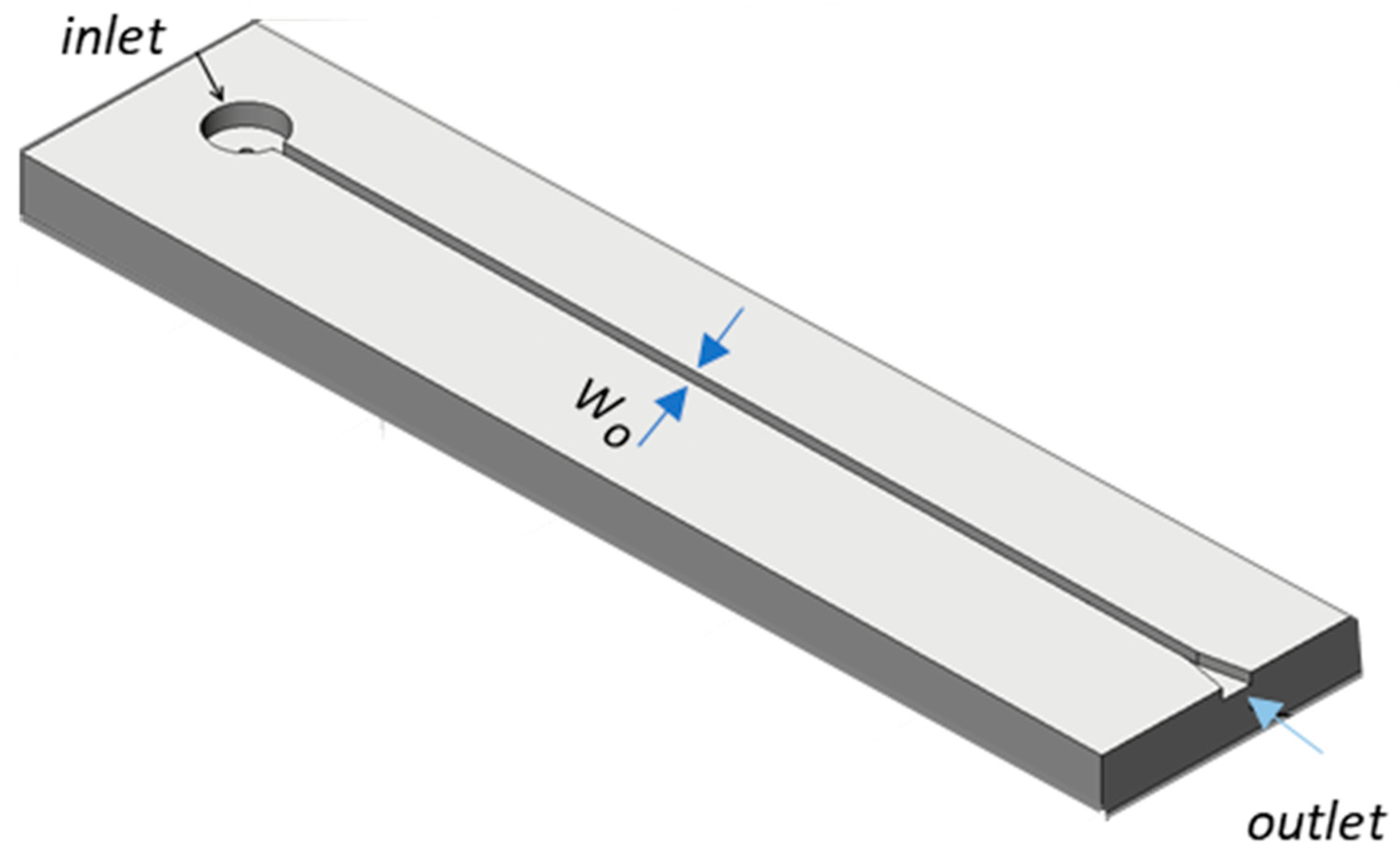
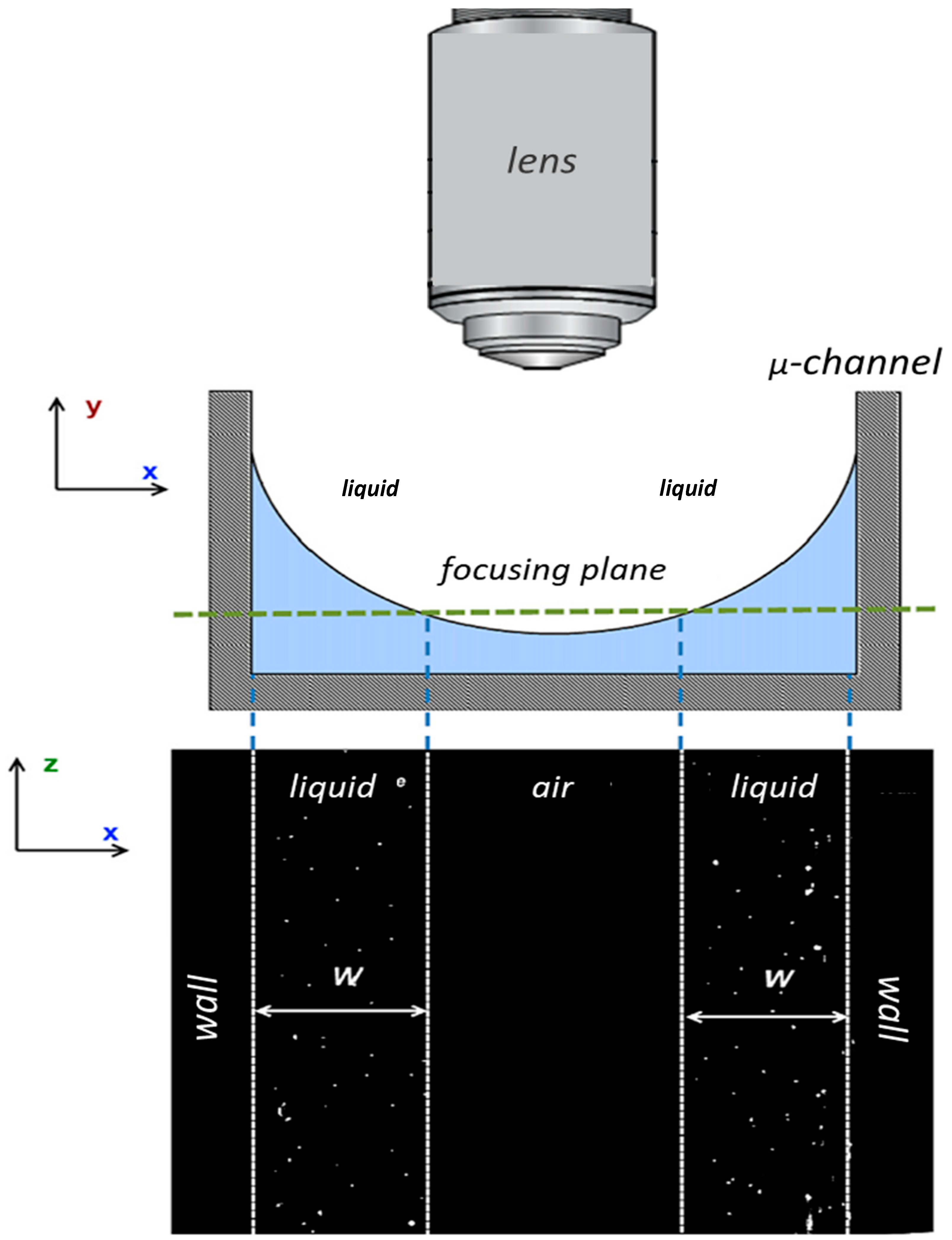
2.1. Experimental Setup
2.2. Measuring Procedure
3. Results and Discussion
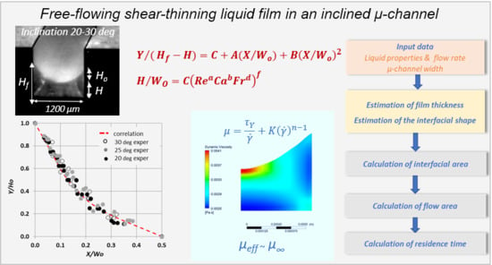
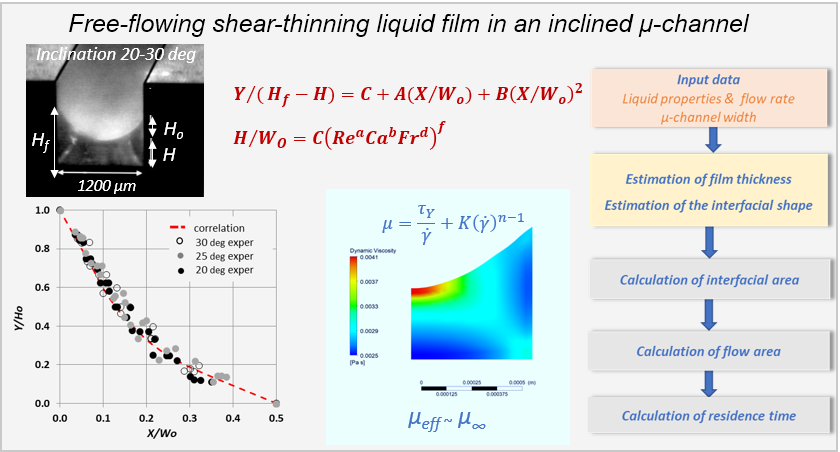
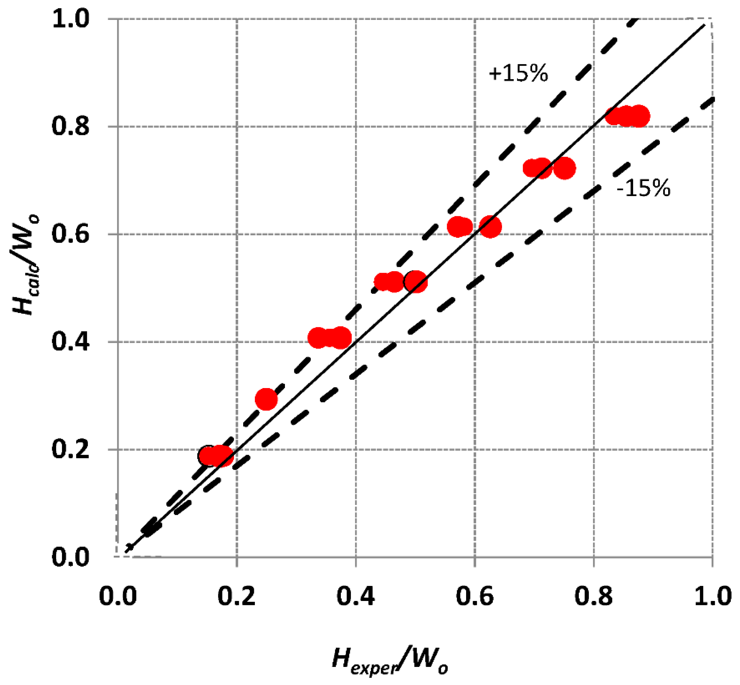
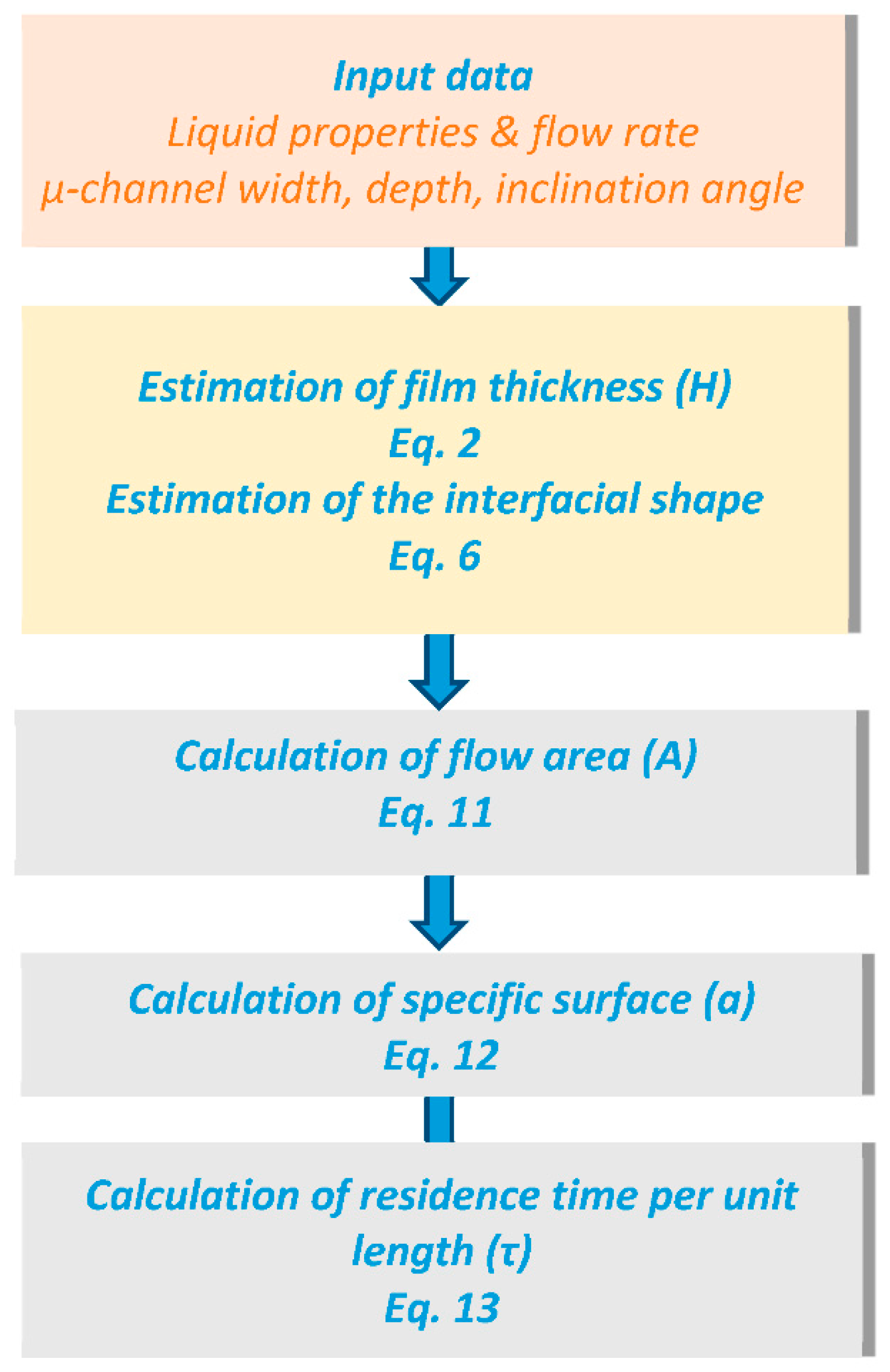
3.1. Liquid Film Thickness Calculation
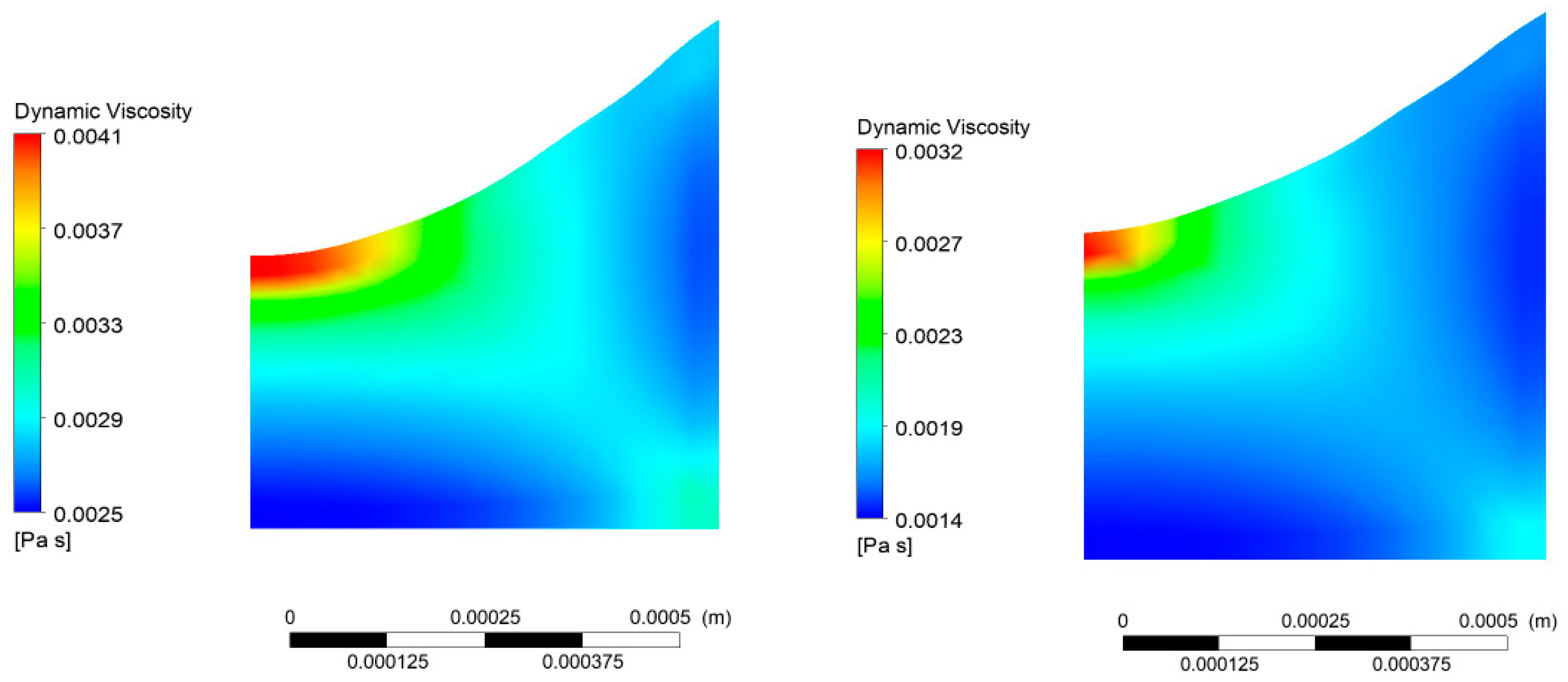
3.2. Effective Viscosity Prediction
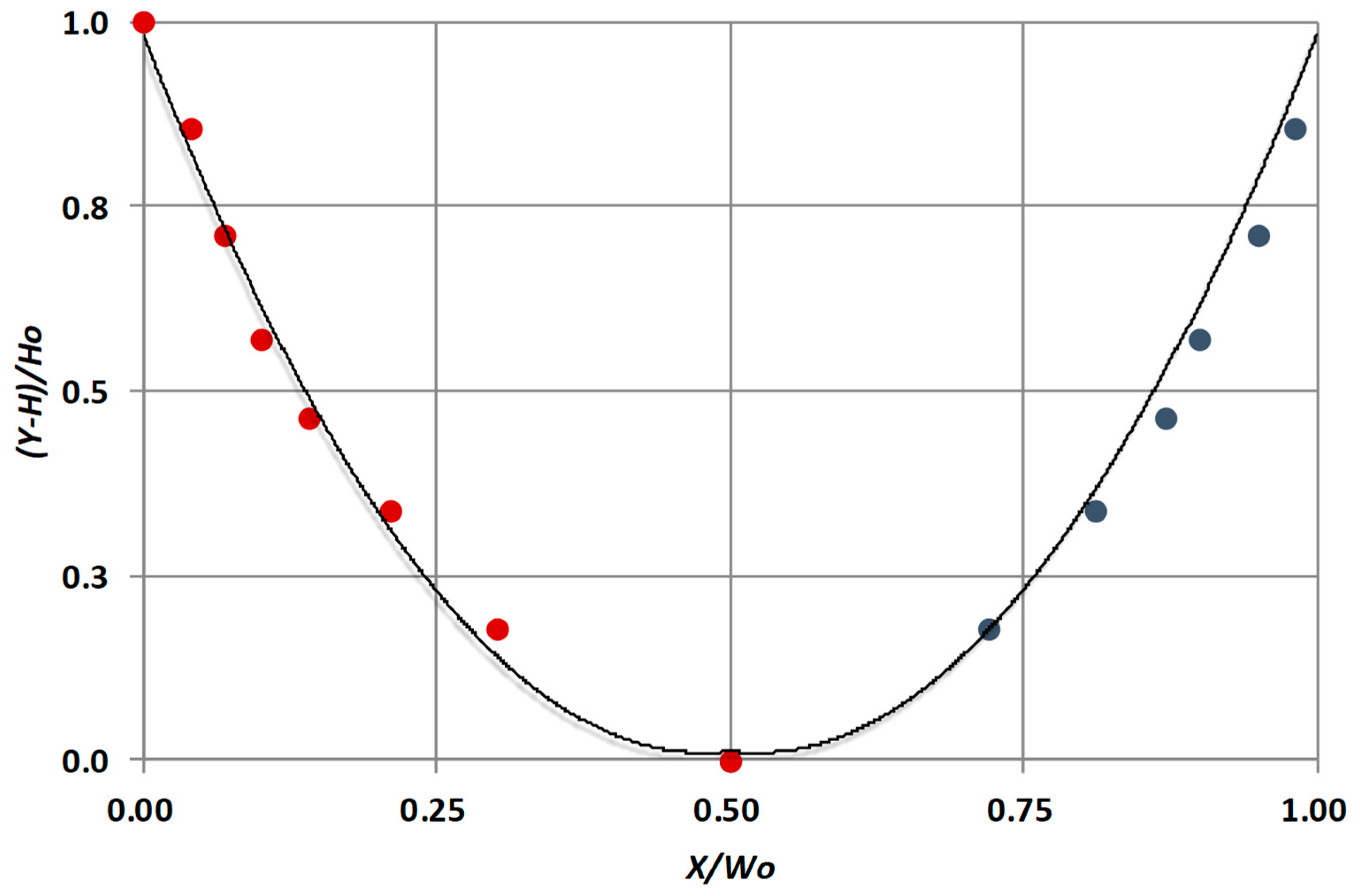
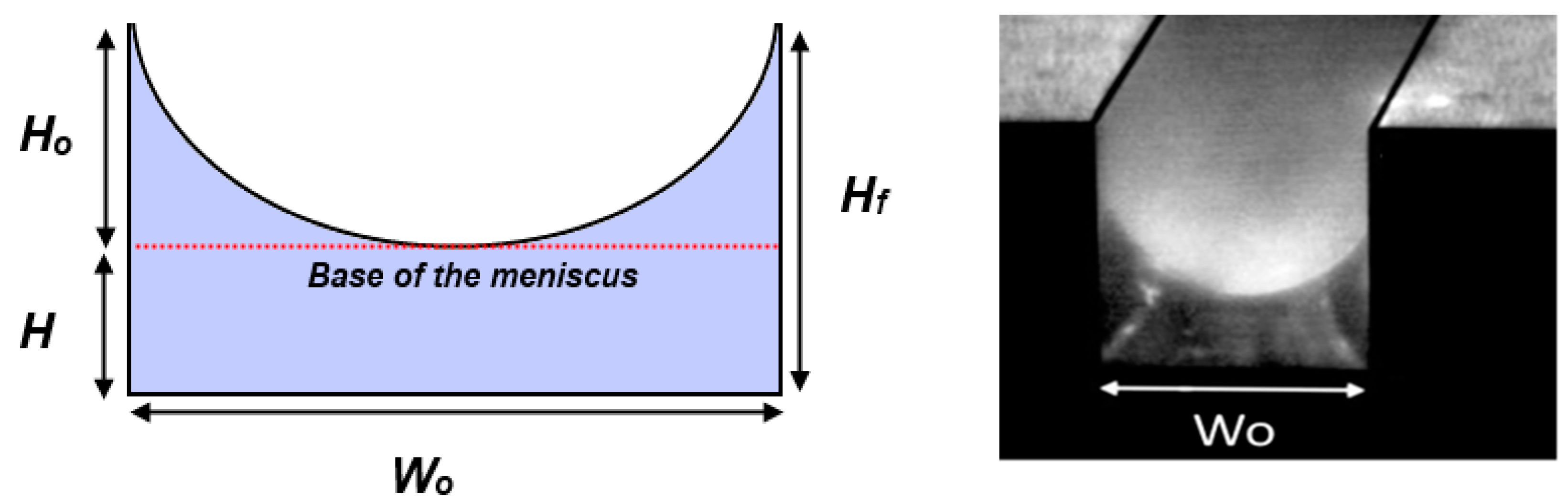
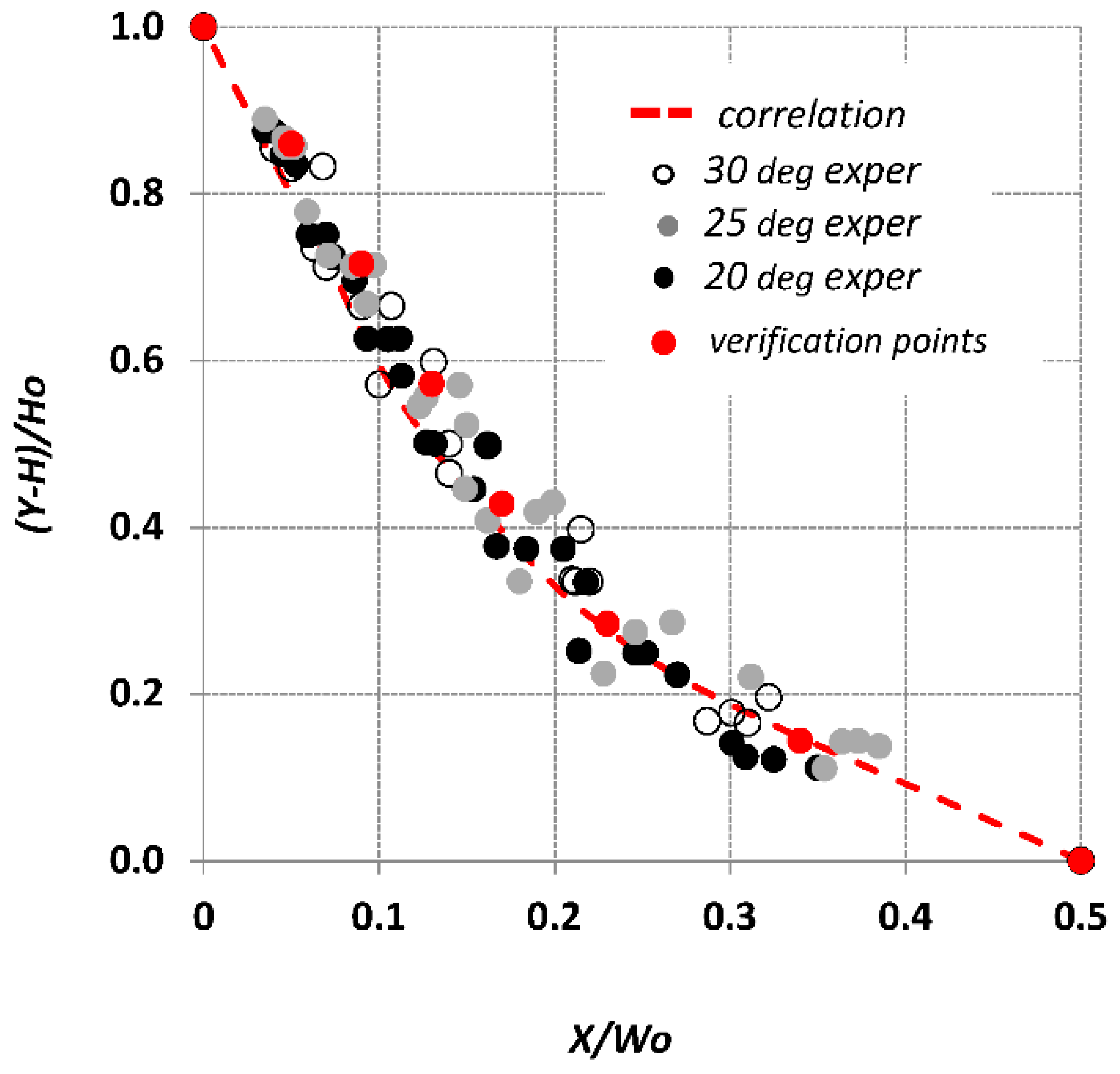
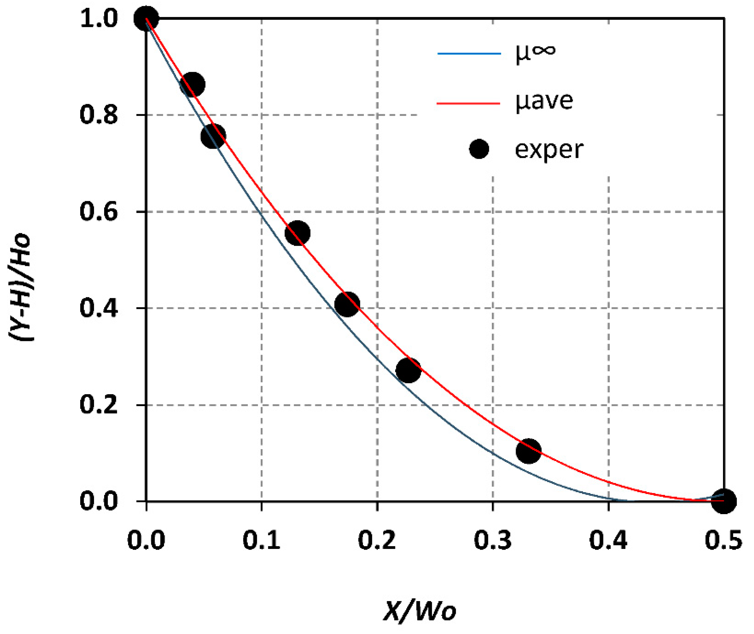
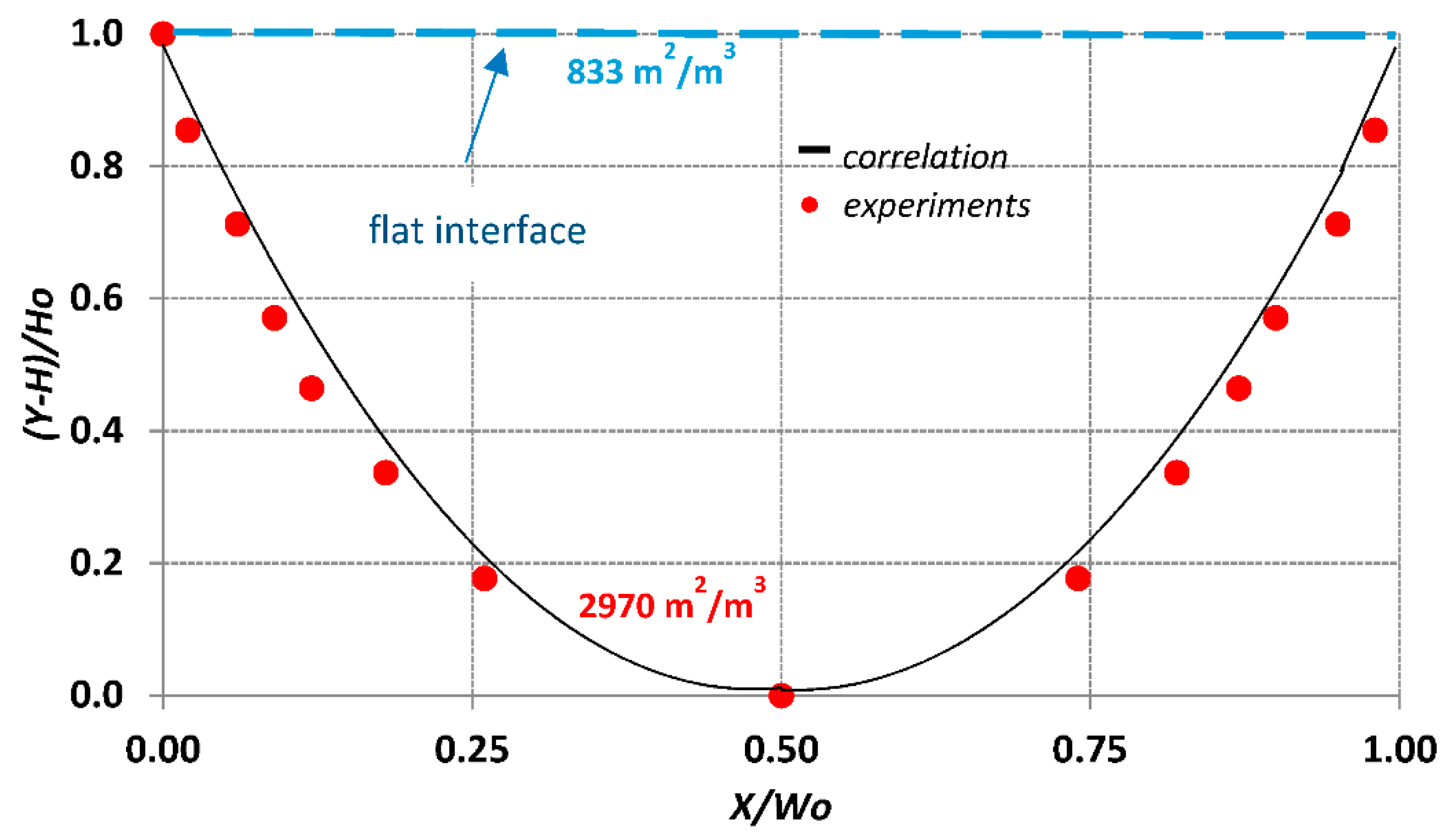
3.3. Meniscus Shape
4. Conclusions
Author Contributions
Funding
Acknowledgments
Conflicts of Interest
Nomenclature
| A | liquid phase cross section | μm2 |
| Ca | capillary number | Dimensionless |
| Fr | Froude number | Dimensionless |
| g | acceleration of gravity | m/s2 |
| Hf | height of the microchannel | μm |
| Ho | height of the meniscus | μm |
| H | liquid film thickness | μm |
| L | length of the interface (meniscus) | μm |
| M | objective lenses magnitude | Dimensionless |
| m | mass flow rate | kg/s |
| NA | numerical aperture | Dimensionless |
| Q | volumetric flow rate | mL/h |
| Re | Reynolds number | Dimensionless |
| S | gas–liquid interfacial area | μm2 |
| V | total fluid volume | μm3 |
| X | distance from vertical wall | μm |
| Y | distance from the channel bottom | μm |
| WO | width of microchannel | μm |
| Greek symbols | ||
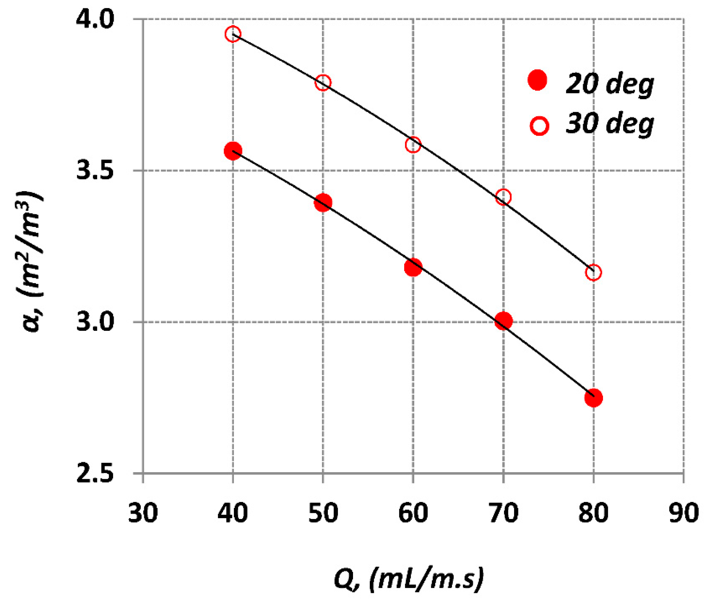
| α | specific surface | m2/m3 |
| μ | liquid viscosity | Pa·s |
| σ | surface tension | N/m |
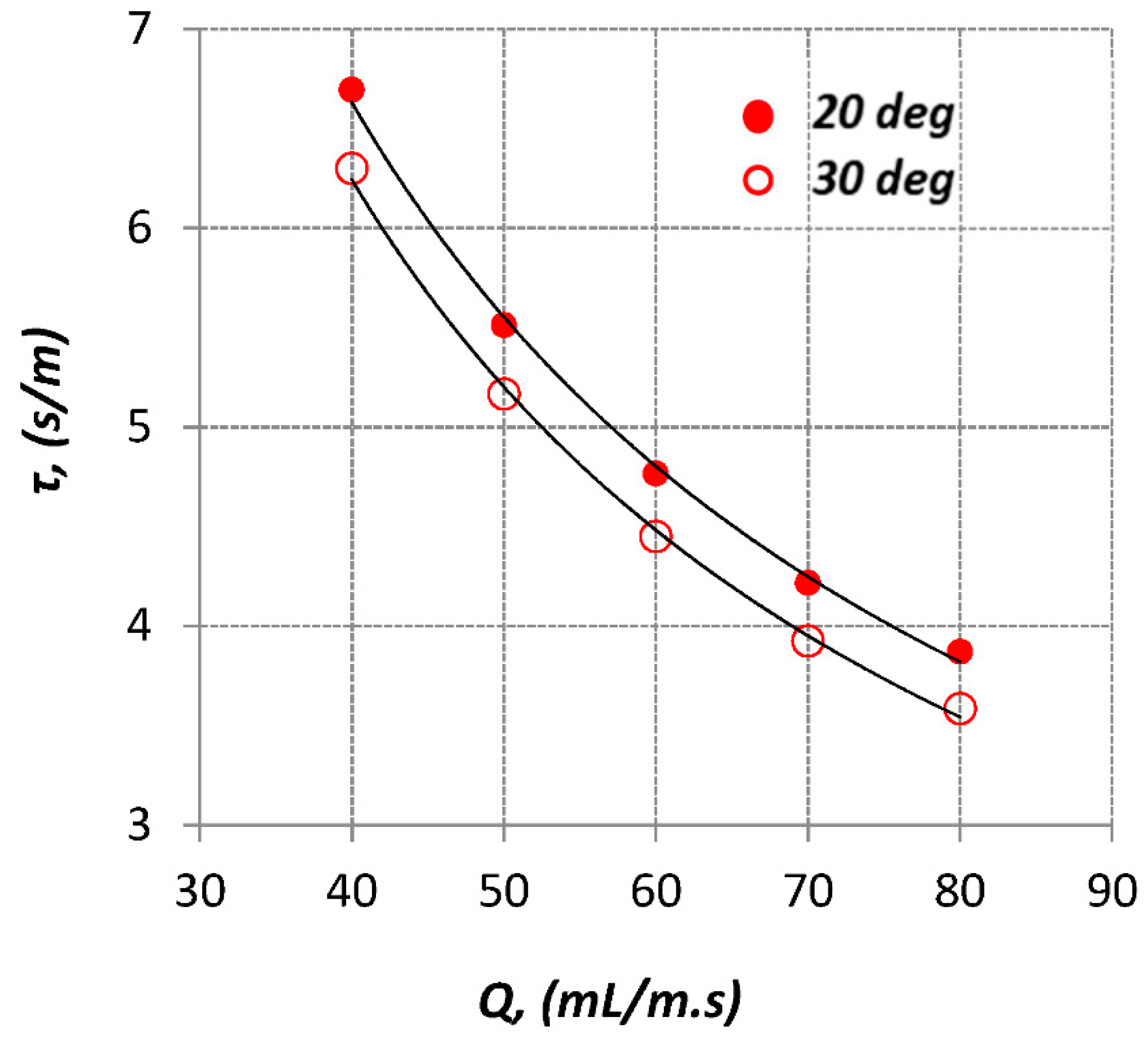
| τ | residence time/channel length | s/m |
| ρ | liquid density | kg/m3 |
| φ | inclination angle | ° |
References
- Sackmann, E.K.; Fulton, A.L.; Beebe, D.J. The present and future role of microfluidics in biomedical research. Nature 2014, 507, 181–189. [Google Scholar] [CrossRef] [PubMed]
- Yetisen, A.K.; Akram, M.S.; Lowe, C.R. Paper-based microfluidic point-of-care diagnostic devices. Lab Chip 2013, 13, 2210–2251. [Google Scholar] [CrossRef] [PubMed]
- Hessel, V.; Löwe, H.; Schönfeld, F. Micromixers—A review on passive and active mixing principles. Chem. Eng. Sci. 2005, 60, 2479–2501. [Google Scholar] [CrossRef]
- Chambers, R.D.; Holling, D.; Spink, R.C.; Sandford, G. Elemental fluorine. Part 13. Gas-liquid thin film microreactors for selective direct fluorination. Lab Chip 2001, 1, 132–137. [Google Scholar] [CrossRef] [PubMed]
- Stavarek, P.; Le Doan, T.V.; Loeb, P.; De Bellefon, C. Flow visualization and mass transfer characterization of falling film reactor. In Proceedings of the 8th World Congress of Chemical Engineering, Montreal, QC, Canada, 23–27 August 2009. [Google Scholar]
- Tourvieille, J.-N.; Bornette, F.; Philippe, R.; Vandenberghe, Q.; de Bellefon, C. Mass transfer characterisation of a microstructured falling film at pilot scale. Chem. Eng. J. 2013, 227, 182–190. [Google Scholar] [CrossRef]
- Yu, D.; Hu, X.; Guo, C.; Wang, T.; Xu, X.; Tang, D.; Nie, X.; Hu, L.; Gao, F.; Zhao, T. Investigation on meniscus shape and flow characteristics in open rectangular microgrooves heat sinks with micro-PIV. Appl. Therm. Eng. 2013, 61, 716–727. [Google Scholar] [CrossRef]
- Ishikawa, H.; Ookawara, S.; Yoshikawa, S. A study of wavy falling film flow on micro-baffled plate. Chem. Eng. Sci. 2016, 149, 104–116. [Google Scholar] [CrossRef]
- Lokhat, D.; Domah, A.K.; Padayachee, K.; Baboolal, A.; Ramjugernath, D. Gas–liquid mass transfer in a falling film microreactor: Effect of reactor orientation on liquid-side mass transfer coefficient. Chem. Eng. Sci. 2016, 155, 38–44. [Google Scholar] [CrossRef]
- Yang, Y.; Zhang, T.; Wang, D.; Tang, S. Investigation of the liquid film thickness in an open-channel falling film micro-reactor by a stereo digital microscopy. J. Taiwan Inst. Chem. Eng. 2018. [Google Scholar] [CrossRef]
- Patel, R.S.; Garimella, S.V. Technique for quantitative mapping of three-dimensional liquid–gas phase boundaries in microchannel flows. Int. J. Multiph. Flow 2014, 62, 45–51. [Google Scholar] [CrossRef]
- Anastasiou, A.D.; Makatsoris, C.; Gavriilidis, A.; Mouza, A.A. Application of μ-PIV for investigating liquid film characteristics in an open inclined microchannel. Exp. Therm. Fluid Sci. 2013, 44, 90–99. [Google Scholar] [CrossRef]
- Anastasiou, A.D.; Gavriilidis, A.; Mouza, A.A. Study of the hydrodynamic characteristics of a free flowing liquid film in open inclined microchannels. Chem. Eng. Sci. 2013, 101, 744–754. [Google Scholar] [CrossRef]
- Chhabra, R.P.; Richardson, J.F. Non-Newtonian Flow and Applied Rheology: Engineering Applications; Butterworth-Heinemann: Oxford, UK, 2011; ISBN 978-0-08-095160-7. [Google Scholar]
- Anastasiou, A.D.; Al-Rifai, N.; Gavriilidis, A.; Mouza, A.A. Prediction of the characteristics of the liquid film in open inclined micro-channels. In Proceedings of the 4th Micro and Nano Flow Conference 2014, London, UK, 6–10 September 2014. [Google Scholar]
- Spiegel, M.R.; Liu, J. Mathematical Handbook of Formulas and Tables; McGraw-Hill: New York, NY, USA, 1999; ISBN 978-0-07-038203-9. [Google Scholar]


| Index | Liquid | Refractive Index | Contact Angle | Density | Surface Tension | Viscosity |
|---|---|---|---|---|---|---|
| - | (°) | (kg/m3) | (mN/m) | (Pa·s) | ||
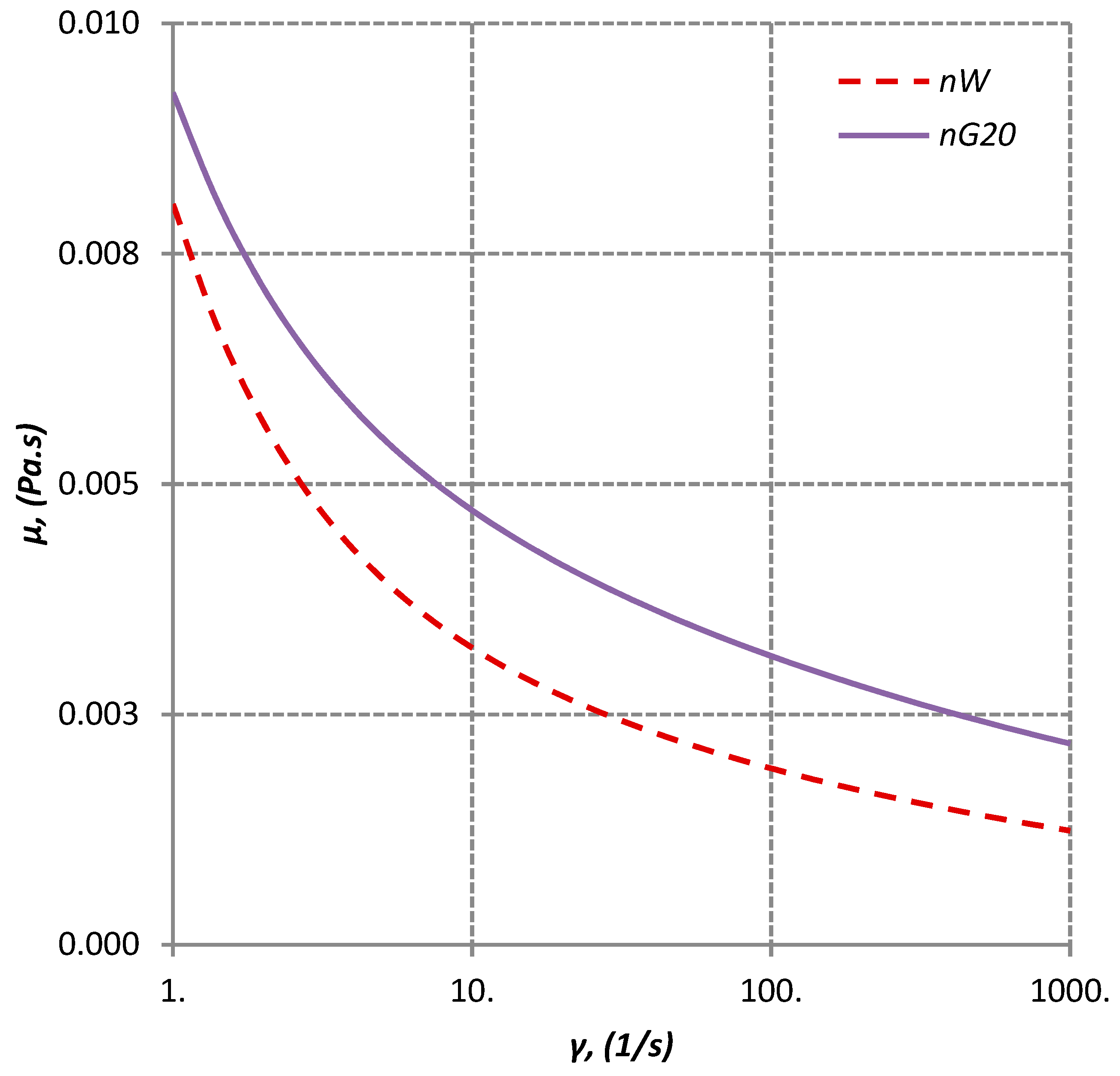
| nW | 100% water + 0.03% xanthan gum | 1.340 | 74 | 998 | 72.1 | μ = 0.003698γ−1 + 0.004339γ−0.1819 |
| nG20 | 75% water + 25% glycerol w/w + 0.03% xanthan gum | 1.360 | 74 | 1059 | 66.7 | μ = 0.002952γ−1 + 0.006295γ−0.1535 |
| Fluid | μ∞ (Pa·s) | μave (Pa·s) | % Difference |
|---|---|---|---|
| nG20_80 | 0.0025 | 0.00260 | 4.0 |
| nG20_40 | 0.0025 | 0.00270 | 8.0 |
| nW_80 | 0.0014 | 0.00145 | 4.0 |
| nW_40 | 0.0014 | 0.00150 | 7.1 |
| Constants for Equation (1) | Present Work | Previous Work [13] |
|---|---|---|
| a | 0.50 | 0.50 |
| b | 0.01 | 0.01 |
| c | 3.90 | 2.04 |
| d | −0.56 | −0.56 |
| f | −0.86 | −0.86 |
© 2019 by the authors. Licensee MDPI, Basel, Switzerland. This article is an open access article distributed under the terms and conditions of the Creative Commons Attribution (CC BY) license (http://creativecommons.org/licenses/by/4.0/).
Share and Cite
Koupa, A.T.; Stergiou, Y.G.; Mouza, A.A. Free-Flowing Shear-Thinning Liquid Film in Inclined μ-Channels. Fluids 2019, 4, 8. https://doi.org/10.3390/fluids4010008
Koupa AT, Stergiou YG, Mouza AA. Free-Flowing Shear-Thinning Liquid Film in Inclined μ-Channels. Fluids. 2019; 4(1):8. https://doi.org/10.3390/fluids4010008
Chicago/Turabian StyleKoupa, Angeliki T., Yorgos G. Stergiou, and Aikaterini A. Mouza. 2019. "Free-Flowing Shear-Thinning Liquid Film in Inclined μ-Channels" Fluids 4, no. 1: 8. https://doi.org/10.3390/fluids4010008
APA StyleKoupa, A. T., Stergiou, Y. G., & Mouza, A. A. (2019). Free-Flowing Shear-Thinning Liquid Film in Inclined μ-Channels. Fluids, 4(1), 8. https://doi.org/10.3390/fluids4010008