1. Introduction
Despite the great advances in reservoir modeling tools and the advent of high-performance computing, high-fidelity physics based numerical simulation still remains a challenging step in understanding the physics of the reservoir and the relationship between the model parameter and control inputs for improved recovery efficiency. History matching, optimization, and uncertainty quantification, which are instances of computationally intensive frameworks, become impractical in a timely manner if real-time data needs to be integrated into the model. Also, the computational time of such large-scale models becomes a bottleneck of fast turnarounds in the decision-making process.
Although there have been a lot of efforts on the traditional CO
2-enhanced oil recovery (EOR) modeling and optimization of the water-alternating-gas (WAG) cycles and well controls [
1], the building of the reduced order models for this phenomenon has not gained as much attention.
The objective in this work is to describe the surrogate reservoir model (SRM) procedure that can be used in the context of computational production optimization. A strategic requirement for any such technique is the ability to provide very fast, yet sufficiently accurate, simulation results.
Within the context of reservoir simulation, a surrogate model is a mathematical model that can approximate the output of a simulator for a set of input parameters or alternate a given physical model. A useful surrogate model should be sufficiently accurate for the problem at hand, while requiring significantly less computational effort than the full-order simulation.
A surrogate can be made using different methods, such as data regression; machine learning; reduced order modeling; reduced physics modeling, which includes coarsening of the model in spatial and time dimensions; and lower order discretization methods [
2].
In all the proxy modeling methods briefly explained in this section, an approximation or simplification is taking place. These techniques can be divided into statistical and mathematical models based on their approach and each will have sub-categories. Examples of proxy models based on a statistical approach are response surfaces or the methods that are based on correlations/causalities or predetermination of functional form. Reduced order models (ROMs) and upscaling techniques fall within the category of the mathematical proxy models. Current model reduction techniques can be categorized into intrusive and non-intrusive methods depending on whether construction of the reduced order model requires knowledge and modification of the governing equations and numerical implementation of the full-fledged simulator. Intrusive ROMs are not applicable when the source code is inaccessible, which is the case for most commercial simulators. The other problem with most current proxy models is that by increasing the number of inputs, the number of trainings needs to increase sharply, as sampling is required to cover the input parameter space. The “curse of dimensionality” challenges the common ROMs used [
3].
The other approaches for categorizing the proxy modeling applied in the realm of reservoir simulation are essentially based on the three categories of response surface models, reduced-physics models, and reduced-order models [
4].
While there have been some methods used for well-based proxy modeling, there are very limited techniques available in the literature focused on grid-based proxy modeling for a black-oil reservoir model, let alone the compositional simulations. These methods have stern pitfalls and drawbacks.
Zhang and Sahinidis [
5,
6,
7] used polynomial chaos expansion (PCE) to build a proxy model, which is used for uncertainty quantification and injection optimization in a carbon sequestration system. The defined model is a 2-D homogenous and isotopic saline formation, with 986 gridblocks. Quantifying the impact of the uncertain parameters (porosity and permeability) on the model outputs (pressure and gas saturation) were of interest. In total, 100 simulation runs were performed in order to build PCEs of an order of (
d = 3 or 4). Since the coefficients in the PCE model are dependent on space and time, this process involves generating a large number of PCE models. As the number of inputs (uncertain parameters) increases, the number of numerical runs needed sharply grows which makes this approach impractical, e.g., at least 8008 runs are required in the case of having 8 inputs and PCE of order 6. The runtime of seconds for PCE and 15 min for numerical simulation has been reported, while it should be noted that each PCE provides the information only in one gridblock and a specific time whilst the numerical simulation provides the results at all the time steps and gridblocks. The contours of gas saturation could not be simulated precisely even after smoothing.
Van Doren et al. proposed reduced order modeling for production optimization in a waterflooding process by use of proper orthogonal decomposition (POD) [
8]. They constructed the ROM using the data obtained from many snapshots of the model states (pressure and water saturation distribution) from the full order simulation model. The POD was used to summarize the dynamic variability of the full order reservoir model in a reduced subspace. Although the number of state vectors (containing oil pressures,
, and water saturations,
, for each gridblock) is decreased using POD, a change in the matrix structure from penta-diagonal (or hepta-diagonal in 3-D systems) to a full matrix counteracts the computational advantage obtained by vector size reduction. In general, although the POD methodology yields reduced-order models with low complexity, the actual speed up on the simulation is modest as compared with the size of the models. The main drawbacks of the POD stem from the fact that the projection basis is dependent upon the training inputs and the time scale that the snapshots are taken.
Cardoso and Durlofsky [
9] emphasized that for nonlinear problems, the POD procedure is limited in terms of the speed up it can achieve, because it targets only the linear solver and the computation effort for some of the operations (constructing the full residual and Jacobian matrices at every iteration of every time step) is not reduced. These authors applied a trajectory piecewise linearization process to the governing equations in addition to the reduced order model obtained from the POD projection and incorporated it in production optimization. The process under the study was waterflooding in a 3-D model having 20,400 gridblocks and 6 wells (4 producers and 2 injectors), in which the well bottom hole pressures (BHPs) were altering. Although the final calculations for estimating the new state vectors can be performed fast using this method, the preprocessing calculations, including running some number of high fidelity training simulations, the construction of the reduced basis function, construction and inversion of the reduced Jacobian matrix for all saved states, construction of a reduced representation of states, accumulation matrix, and source/sink term matrix of derivatives, is still computationally costly. On the other hand, the accuracy of the trajectory piecewise linearization (TPWL) solution is sensitive to the number of basis vectors used in the projection matrix; therefore, some amount of numerical experimentation may be required to establish these numbers for saturation and pressure. Instabilities and a deterioration of accuracy due to the application of the procedure to control inputs far away from the training trajectories are one of the main drawbacks of TPWL [
10].
One application of proxy models is for dealing with the compositional simulation. These simulations are required for modeling the EOR, CO2 sequestration, or gas injection. Due to the intrinsic nonlinearity of these models and the potentially large system of unknowns, they can demand high computational powers. Especially for production optimization, hundreds or thousands of simulation runs should be performed, which accentuates how imperative it is that a model runs efficiently.
Proxy models sometimes have been used as a term just to represent correlations or simple mathematical models to provide single outputs. In one of these applications, oil recovery of a reservoir after carbon dioxide flooding has been modeled as a hint for reservoir screening. The reservoir models used in this study are simple homogeneous models (except in permeability), which differ in the type of reservoir fluid [
11].
Yang et al. have used a hybrid modeling technique for reservoir development using both full-physics and proxy simulations [
12]. The proxy model used in their work is a profile generator. It simplifies the reservoir into material balance tanks and well source/sink terms into a set of tables known as type curves, which relates production gas-to-oil ratio (GOR), water cut, etc. to estimated ultimate recovery (EUR) and other parameters. The main assumption is that the reservoir is to be operated in a way not significantly different from the base case for which the type curve data is produced, which might not be practical in most real field problems.
In another attempt of using proxy models, NRAP (National Risk Assessment Partnership) has focused on using this tool for long-term quantitative risk assessment of carbon storage [
13]. This is performed by dividing the carbon storage system into components (reservoir, wells, seals, groundwater, and atmosphere), using proxy models for each component, and integrating all the models to assess the success probability of carbon storage using the Monte Carlo simulation. Different proxy models are used, including look-up table (LUT), response surface, PCE, and artificial intelligence (AI)-based surrogate reservoir models. The look up table methodology is very simple, but requires hundreds of runs of the high-fidelity model based on different inputs. Although this method is quite rapid, the problem lies in the number of the full-physics model simulations needed to build the table. In the work performed by NRAP, for a 2-D, 2-phase (saline formation) model with 10,000 gridblocks, and only three variable parameters of reservoir permeability, reservoir porosity, and seal permeability, more than 300 runs were needed to build a table for predicting the pressure and saturation at each gridblock. A heterogeneous field cannot be used in this approach and permeability must be varied through a scalar multiplier. Different time snapshots were selected in the interval of 1000 years of post-injection. The size of the look up table and accuracy of the model depends on the selected snapshots and the time span between them.
Data driven modeling sometimes has been used in combination with other reduced order modeling techniques. Klie used a non-intrusive model reduction approach based on POD, discrete empirical interpolation method (DEIM), and radial basis functions (RBFs) networks to predict the production of oil and gas reservoirs [
14]. POD and DEIM helped to project the matrices from a high dimensional space to a low dimensional one. The DEIM method has a complexity proportional to the number of variables in the reduced space. In contrast, POD shows a complexity proportional to the number of variables in the high-dimensional space. POD and DEIM can work as a sampling method for preparing the RBF network input. In this work, a space-filling strategy was used to build the realizations. The permeability in one and the permeability and injection rate in another model were the control variables of the model.
Surrogate reservoir models are approximations of the high-fidelity reservoir models that are capable of accurately mimicking the behavior of the full field models as a function of the changes to all the involved input parameters (reservoir characteristics and operational constraints) in seconds. SRM integrates reservoir engineering and reservoir modeling with machine learning and data mining.
Mohaghegh describes SRM as an “ensemble of multiple, interconnected neuro-fuzzy systems that are trained to adaptively learn the fluid flow behavior from a multi-well, multilayer reservoir simulation model, such that they can reproduce results similar to those of the reservoir simulation model (with high accuracy) in real-time” [
15]. Since 2006, SRM as a rapid replica of a numerical simulation model with quite high accuracy has been applied and validated in different case studies [
16,
17,
18,
19,
20,
21,
22]. SRM can be categorized in well-based [
17,
18,
19,
21,
23] or grid-based types [
16,
20,
24] depending on the objective or the output of the model. In a well-based SRM, the objective is to mimic the reservoir response at the well location in terms of production (or injection). The grid-based SRM, on the other hand, makes it possible to simulate any dynamic properties, such as pressure, phase saturations, or the composition of fluid components, at any specific time or location (gridblock) of the reservoir. This concept has been applied in this research to integrate a grid-based and a well-based surrogate reservoir model for the first time. The developed model is applied to predict the dynamic reservoir properties and production of wells in a reservoir going under water alternative gas (WAG)-EOR, using limited number of reservoir realizations, hence saving significant run-time.
2. Materials and Methods
Injection of CO2 into oil reservoirs can improve oil recovery and at one go alleviate the issue of increased CO2 concentration in the atmosphere. The fact that in most reservoir conditions, CO2 is in a supercritical state makes it a great choice as an enhanced oil recovery (EOR) fluid, due to its high solvency power to extract hydrocarbon components and displace oil miscibly in that state.
2.1. Field Background
The Kelly-Snyder field, discovered in 1948, is one of the major oil reservoirs in the US. The original estimate of its original oil in place (OOIP) was approximately 2.73 billion bbls. The primary production mechanism was indicated as merely solution gas drive, based on the early performance history of the field, which would probably result in an ultimate recovery of less than 20% of the OOIP. The SACROC (Scurry Area Canyon Reef Operators Committee) Unit was formed in 1953, and in September 1954, a massive pressure maintenance program was started. Based on this plan, water was injected into a center-line row of wells along the longitudinal axis of the reservoir [
25].
In 1968, a technical committee, studying potential substitutes, suggested that a water-driven slug of CO
2 be used to miscibly displace the oil in the non-water-invaded portion of the reservoir. CO
2 injection was begun in early 1972. An inverted nine-spot miscible flood program, consisting of injecting CO
2, driven by water was decided to be the most effective and economical alternative method for improving recovery based on the investigations [
25].
SACROC has undergone CO
2 injection since 1972 and is the oldest continuously operated CO
2-EOR operation in the United States. The amount of injected CO
2 until 2005 was about 93 million tones (93,673,236,443 kg), out of which about 38 million tones (38,040,501,080 kg) had been produced. Accordingly, a simple mass balance suggests that about 55 million tones (55,632,735,360 kg) of CO
2 have been accumulated in the site [
26]. In 2000, the production, which once was more than 200,000 bbls/day, had declined to 8200 bbl/day. SACROC continues to be flooded by the current owner/operator, Kinder Morgan CO
2.
After years of CO
2-EOR projects, the industry came to this consensus that the parts in the reservoir that have performed the best and had highest recovery under the waterflood process will also have the best response to CO
2 flooding [
27].
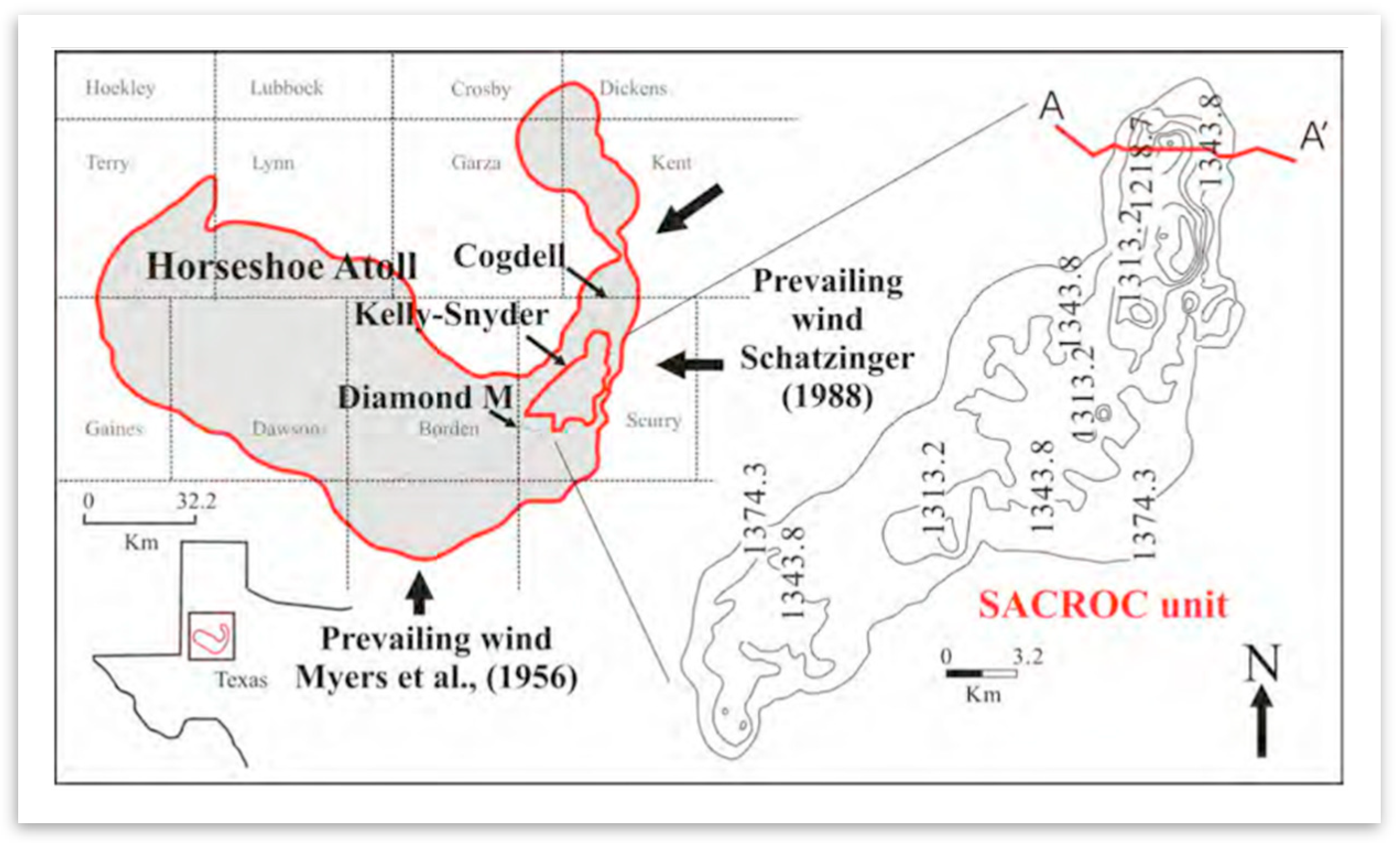
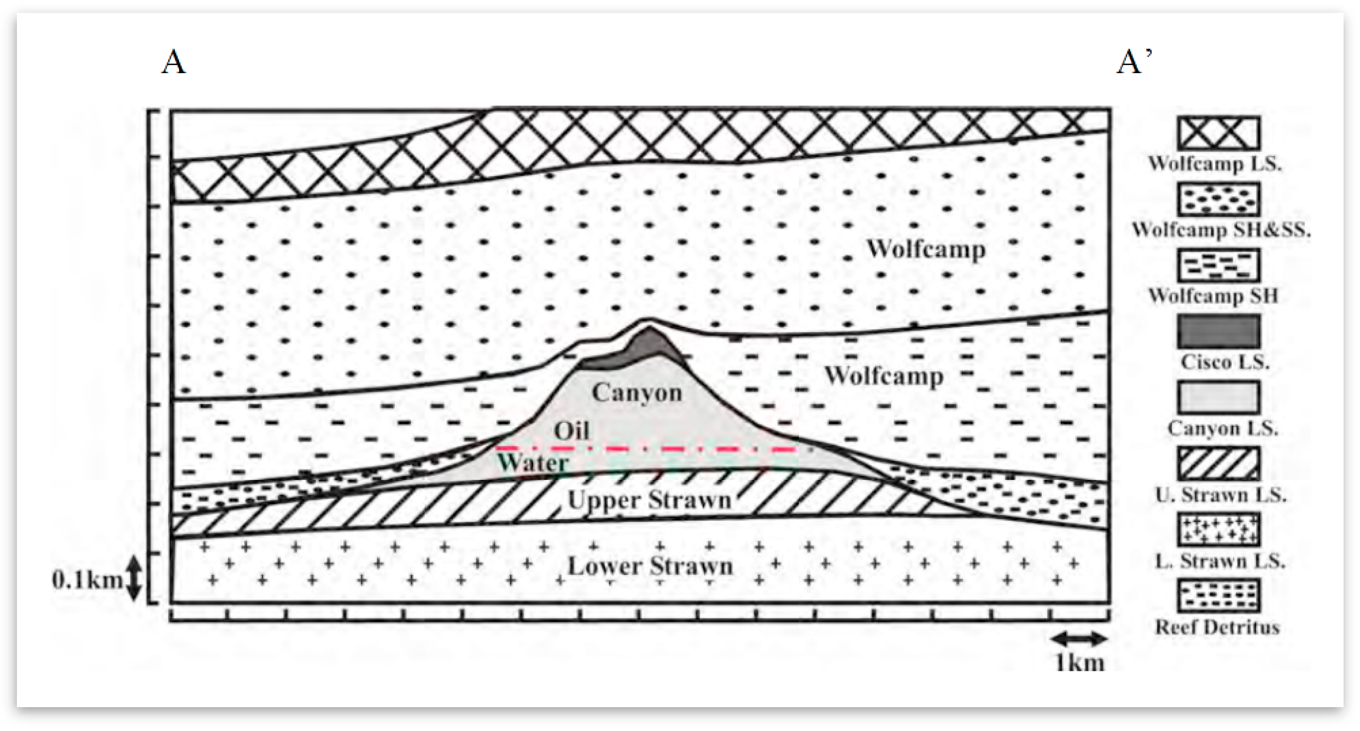
SACROC is located in the southeastern segment of the Horseshoe Atoll within the Midland basin of west Texas (
Figure 1). SACROC covers an area of 356 km
2 with a length of 40 km and a width of 3 to 15 km, within the Horseshoe Atoll. Geologically, massive amounts of bedded bioclastic limestone and thin shale beds representing the Strawn, Canyon, and Cisco formations of the Pennsylvanian, and the Wolfcamp Series of the Lower Permian comprise the carbonate reef complex at SACROC (
Figure 2) [
28]. Among these formations, most of the CO
2 for EOR has been injected into Cisco and Canyon formations, which were deposited during the Pennsylvanian age. Although the Canyon and Cisco formations are mostly composed of limestone, minor amounts of anhydrite, sand, chert, and shale are present locally. The Wolfcamp shale of the lower Permian acts as a seal above the Canyon and Cisco Formations [
29].
2.2. Geo-Cellular Numerical Model
The fine-scale geological model was built [
31]. The top section of the high-resolution model has been used for the works performed in this study. This section consists of 3,138,200 (149 × 100 × 221) fine scale gridblocks. Although the fine-scale geocellular model delivers a quantified characterization of natural heterogeneity in the SACROC northern platform, due to computational limitations, the model had to be upscaled to develop a multi-phase and -species reactive transport model. The upscaling by nature results in less resolution of heterogeneity; however, attempts were made to preserve as much of the heterogeneity as possible.
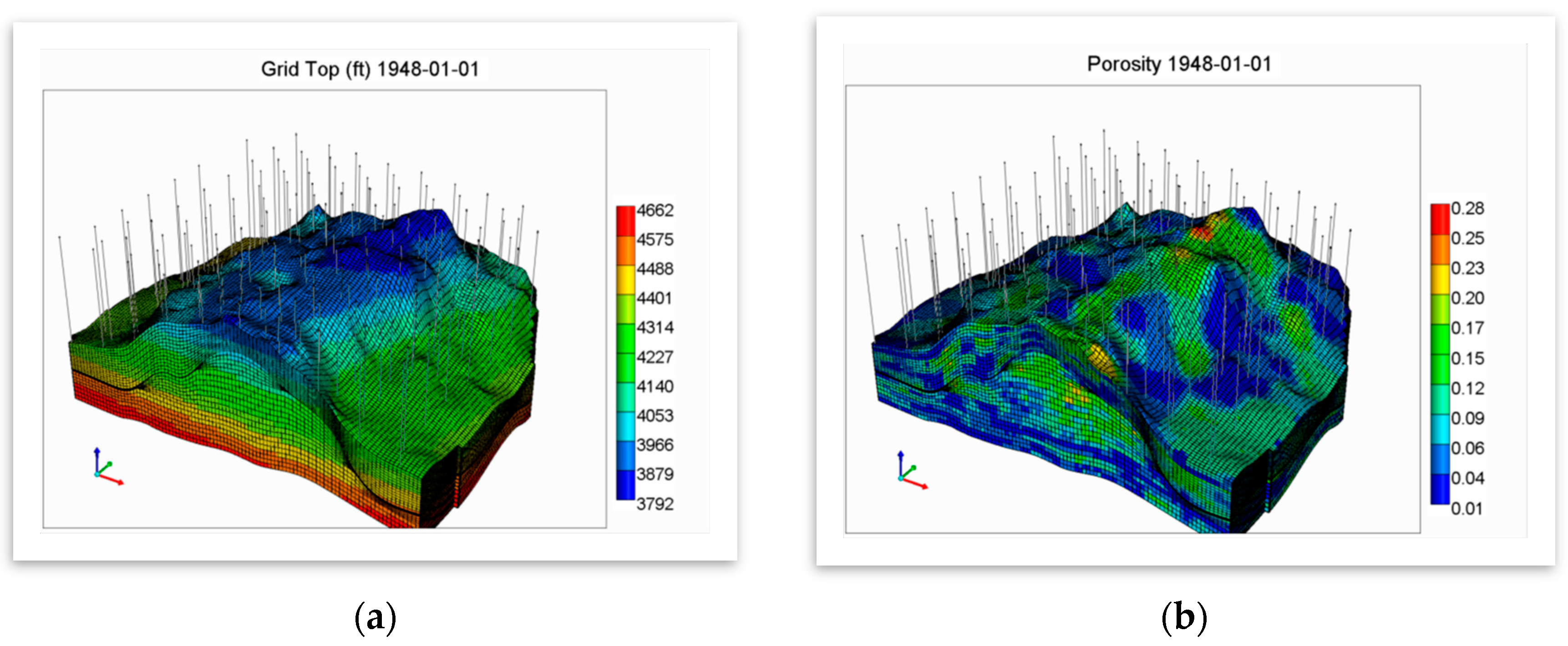
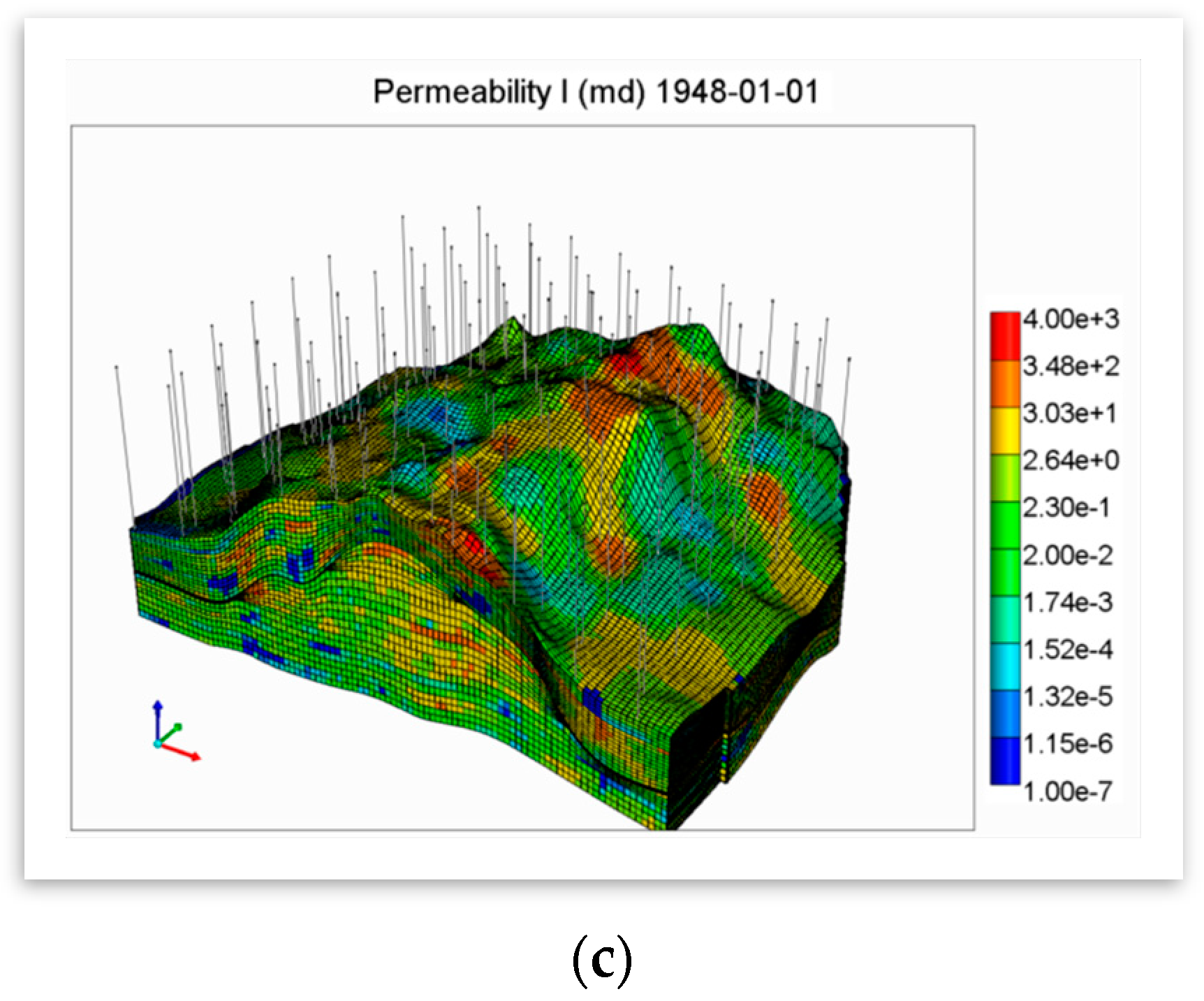
The built geocellular model was transformed to a fluid flow simulation environment, along with the properties’ maps and wells data (
Figure 3). The reservoir model was developed using a commercial reservoir simulator (CMG’s GEM). CMG’s GEM (generalized equation of state model) simulator is a multi-dimensional, finite-difference, isothermal compositional simulator that can simulate three-phase (oil, water, gas) and multicomponent fluids [
32].
The fluid and rock properties were assigned for building the numerical model [
31]. The reservoir section used to build the numerical and SRM has 87 producers. The number of WAG injectors is 39. These wells alternatively inject water and gas in different half cycles. There is a single well, which has been injecting water continuously and has been kept as a water injector. The total amount of oil production in this section of the reservoir (used for this study) is 185 MMstb. The water injection and CO
2 gas injection amount through the history matched period (35 years) is about 519 MMstb and 199 Bscf, correspondingly.
The built numerical model was history matched. The history matching process is very complex, involving a lot of changes due to water and miscible gas injection occurring concurrently with the oil, water, and gas production from multiple wells. This complexity calls for modification of the time steps to small increments to account for drastic pressure or composition, causing very long simulation runs itself while running the simulation. The compositional models by nature take much longer pertaining to the required calculations in comparison with the black oil models. This complexity rises as water injection and later miscible gas injection period starts. The time step size is altering to reach convergence and gets as small as seconds. The total run time for running the model from the beginning of the production (1948) to the end of injection, based on available data (2004), is about 1 month on a machine with 24 GB of RAM and 3.6 GHz CPU.
2.3. SRM Development
The first step in developing SRM is defining a concrete objective. The objective determines the type and scale of SRM. Preparing a spatio-temporal dataset comes next. The developed spatio-temporal database is then used to teach the SRM (AI-based smart proxy model) the principles of fluid flow through porous media and the complexities of the heterogeneous reservoir represented by the geological model and its impact on the fluid production and pressure changes in the reservoir. The spatio-temporal dataset for SRM is built based on the results from handful realizations of the high-fidelity model. Taking a methodical tactic for designing the runs helps extracting the maximum information while contracting the computational time. The rows of a dataset are records/samples or realizations and the columns represent the features or properties (e.g., porosity, permeability, etc.).
This work tries to build a base for optimization in a specific field; thereby, no change in geological realizations will be considered. This would differ if the objective was history matching or uncertainty analysis. Since infill drilling is out of the picture in the miscible CO2 EOR process in this work, the only factors that could be changed and affect the production amount are the operational constraints. The drawdown pressure at each producer is dependent on its bottom-hole pressure. The more drawdown pressure (difference between reservoir and bottomhole pressure) there is, the higher the production of each well will be. The amount of the gas or water injected is another important factor. Apart from the amount of injected fluid, its duration in each half cycle plays an important role. All this can be added up in the definition of the WAG ratio.
In the setting of statistical sampling, a square grid encompassing sample positions is a Latin square if (and only if) there is only one sample in each row and each column. A Latin hypercube is the generalization of this idea to an arbitrary number of dimensions, whereby each sample is the only one in each axis-aligned hyperplane containing it. For sampling a function of variables, the range of each variable is divided into equally probable intervals. sample points are then located to fulfill the Latin hypercube requirement. This forces all variables to have the same number of divisions . One of the main advantages of Latin hypercube sampling (LHS) over other sampling schemes is its independence of the number of samples from the dimensions (variables). Another advantage is that random samples can be taken one at a time, remembering which samples were taken so far. LHS was used for performing the sampling in this work.
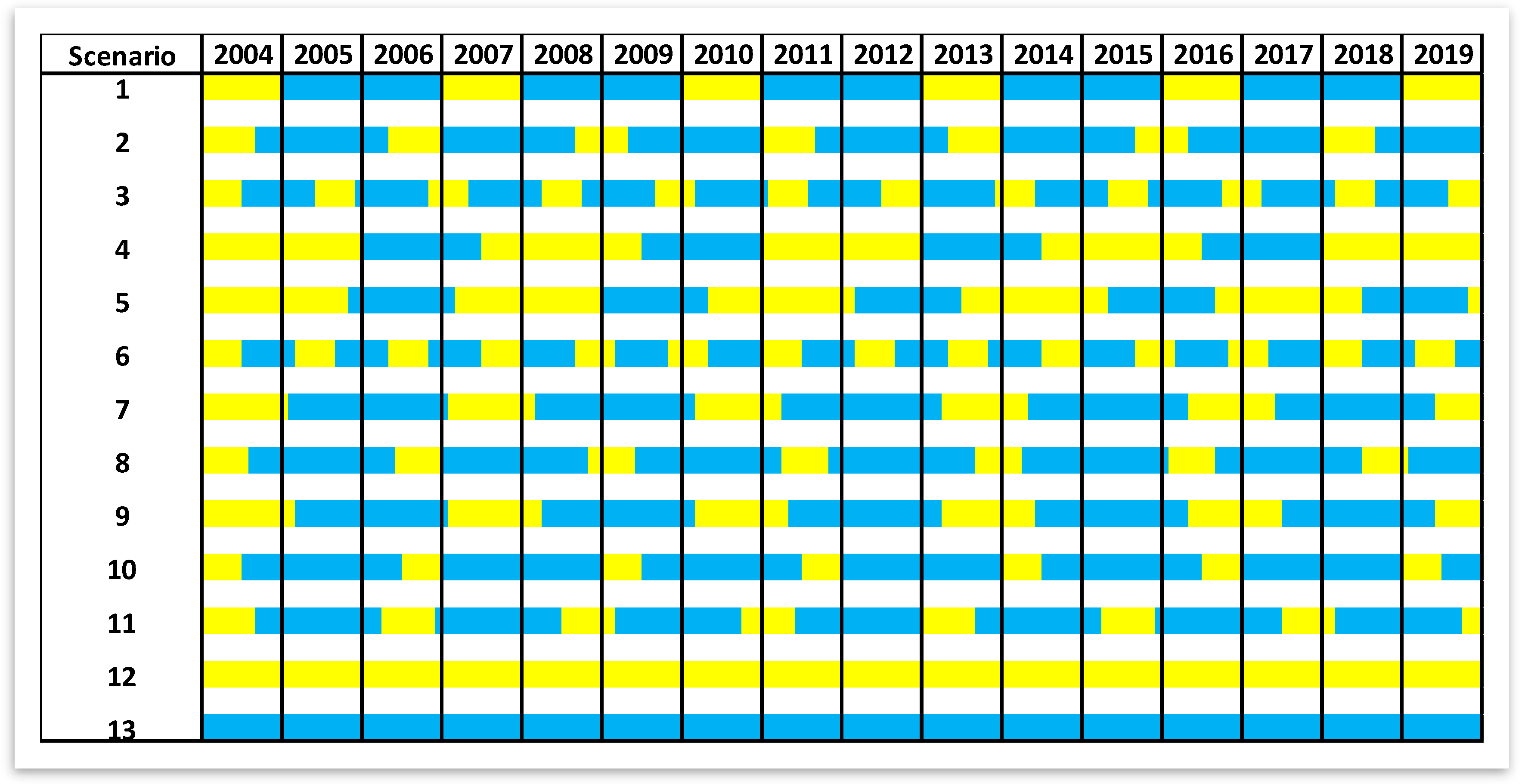
The WAG scenarios were designed based on the sampling of the duration and amount of injection of water and gas as well as the BHP of the production wells. In order to perform the LHS, to generate 11 scenarios, using four variables (water/gas injection rate, injection half cycle duration of water and gas), a minimum and maximum was decided for each variable. The field injection rate is between 10 Mbbl/d and 50 Mbbl/d. The minimum and maximum of the gas injection rate for the field (all WAG wells together) are 10 MMScf/d and 80 MMScf/d. The injection rate was allocated to the wells as their maximum water/gas injection rate constraint, based on their recent performance. Although the constraint was kept constant through the cycles of injection, its value was different in each well. This means that not only the constraint assigned to each well is different from other wells in that scenario, but also it differs from the assigned value of the same well in other scenarios.
Each injection cycle starts with a half cycle of gas injection followed by a half cycle of water injection. The range of these cycles is considered to be 6 months to 24 months (
Figure 4). It was also made sure that the generated scenarios cover the WAG ratio interval of 0.5 to 4.
The BHP at each well at the date of 1 January 2004 was recorded; a random pressure drop between 5% and 30% was applied to this value. The calculated pressure was assigned as the operational constraint (Min BHP) to the production wells in the built scenarios. Using this scheme ensures that the BHP value is unique for each well and it is always greater than the minimum miscibility pressure (MMP). The maximum allowable injection pressure for all the injectors was kept at the constant value of 5000 psi.
On top of the 11 scenarios defined based on the WAG process, two more cases were developed for the situations that exclusively have water or gas for the entire cycle at the highest injection rate.
The described procedure was used to build the scenarios required for developing the SRM. These scenarios differ from each other in terms of the injection scheme of each well (amount and duration of injection) and the operating constraint of the producers.
Table 1 lists these realizations and their corresponding WAG parameter. The initial condition of all the scenarios is the same at 1 January 2004. The built models were run using the numerical simulation.
2.3.1. Grid-Based SRM (SRMG)
Using grid-based SRM, depending on the solicitation of the model, one can estimate properties, such as the pressure, phase saturation, or composition, of reservoir fluid components at any desired time step or gridblock of the reservoir. Grid based SRM is used when there is a specific interest in determining the flood front [
33].
In the current study, the reservoir is going through an alternate water and gas injection, thereby the saturations are drastically changing. The pressure and flood front can be analyzed by generating SRMs that predict pressure, phase saturation, and mole fraction of CO2 at any specific gridblock and time step of the reservoir life. This is vastly useful in performing the optimization and selecting the best injection scenario. In this study, one year has been specified as the desired timestep. The “previous timestep” mentioned in the rest of the article refers to the “previous year”.
SRMG Spatio-Temporal Dataset Generation
A lot of weights in developing an SRM go to the dataset preparation. This dataset is what will be used for teaching the SRM about the reservoir and essentially it should convey the principles of the “physics” of the reservoir and the specific problem at hand. The integrity of output from the SRM is dependent on the integrity of input. Faulty and erroneous data used in a model will result in distorted information. One cannot expect SRM to deliver good results if it has not been taught properly. That is why a reservoir engineering insight is absolutely compulsory for developing an SRM apart from the data mining knowledge.
The structure of the dataset is totally contingent upon the type and the objective of the reservoir.
Table 2 lists the information needed for building the spatio-temporal database used in this study for building the grid-based SRM.
A lumping process was performed to reduce the size of the dataset. This was performed based on the geological zones defined in the geological model. Based on this process, the 36 simulation layers were upscaled to 5 geological zones as shown in
Table 3.
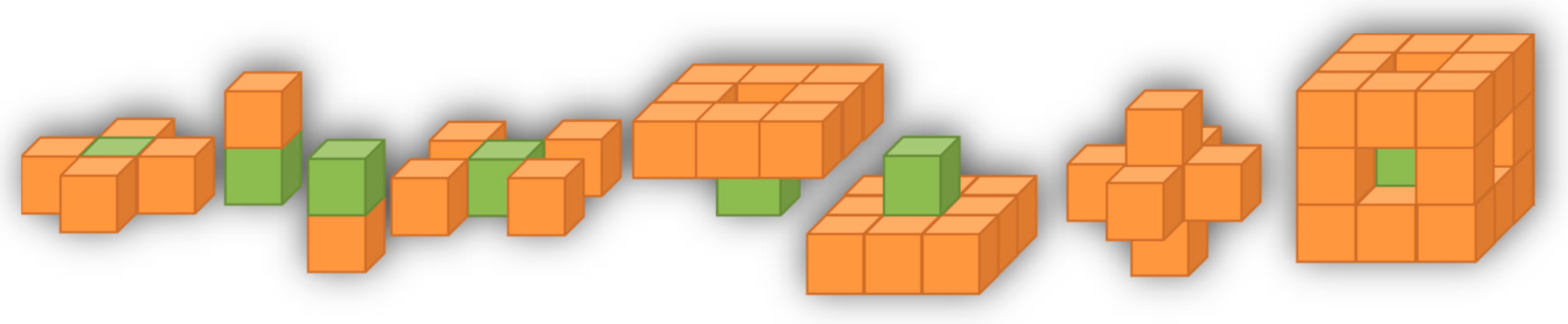
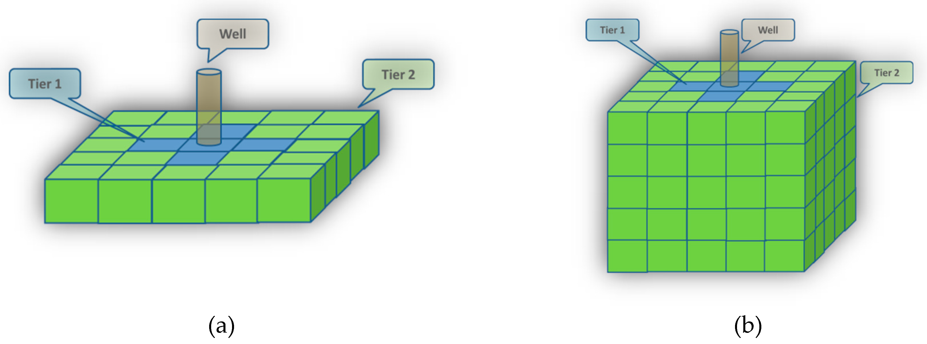
With 100 gridblock in the X direction, 110 gridblocks in the Y direction, and 36 layers (Z direction), there will be 396,000 gridblocks to account for. Since each gridblock can form one record (one row in the database), the lumping process reduces the layers to 5 and causes the size of records in the dataset of one scenario to decrease from 396,000 to 55,000. To consider the impact of surrounding blocks, a tiering system was defined. Each gridblock has 8 corresponding tiers for all the static and dynamic properties. These values vary in time. The values at each tier are the average of properties of the blocks belonging to those tiers using different methods subject to the type of properties being averaged. These methods include arithmetic, weighted arithmetic, and harmonic averaging. The schematic of the tiering system is illustrated in
Figure 5. The blocks assigned to each tier are as follows:
Tier 1: Average of immediate adjacent blocks in the same layer.
Tier 2: Immediate adjacent block in the top layer.
Tier 3: Immediate adjacent block in the bottom layer.
Tier 4: Average of immediate non-adjacent blocks in same layer.
Tier 5: Average of immediate non-adjacent blocks in the top layer.
Tier 6: Average of immediate non-adjacent blocks in the bottom layer.
Tier 7: Average of tier 1, tier 2, and tier 3 values (all adjacent blocks).
Tier 8: Average of tier 4, tier 5, and tier 6 values (all non-adjacent blocks)
The database created from all the training cases will have 650,000 records (having 13 scenarios of 50,000 gridblocks each). The span of potential features can increase over 1000. This is because any static property (such as the location information, distance to offset wells or boundaries, code for type of gridblock, geological properties of the blocks and its associated tier) and dynamic property (such as the pressure, oil or water saturation, CO2 mole fraction of each block and associated tiers at the previous time steps, the static/dynamic properties of the offset production and injection wells for each gridblock and the rate/cumulative volume of each production/injection offset well,…) can be a potential information bearing feature. The number of these features depends on how many tiers is defined, how many offset wells is considered, the results of how many previous timesteps are going to be cascaded into the new timestep, etc. Due to the limitation of the software for handling such a huge dataset, a sampling process should be performed. Through this process, a part of the spatio-temporal database is selected to represent the whole dataset and will be used for the SRM development purpose. As explained before, almost 6% of the whole data records will be extracted using sampling, due to the record limit imposed by the used software.
Different sampling methods were tried on one of the properties and the one with the best results was selected for this study. Some of these methods were as follows:
Method A: Ten percent of data was selected from well locations, 90% of data was randomly selected from the whole data pool.
Method B: The data was ranked according to their pressure values (high pressure to low pressure). Data was then divided in uneven pressure ranges in such a way to have equal records in each created bin (20% of data for each bin).
Method C: The data was ranked according to their pressure values (high pressure to low pressure) and then divided in even pressure ranges (450 psi difference).
Method C was used as the base of sampling.
Table 4 shows the inputs selected out of 310 features for predicting pressure at one of the time steps as an example (pressure network). The properties shown in this table represent the features (columns of dataset), and each row of the dataset represents a gridblock.
Data Partitioning
Selection of the inputs is followed by data partitioning. A random partitioning yields mutually exclusive datasets: A training dataset, a calibration dataset, and a validation dataset. Many times, the success or failure of a project would hinge on how the data is segmented into these portions, or how the entire data set is partitioned. The random partitioning was performed on the dataset to assign 80% of the data (equivalent to 25,600 records) to training, 10% (3200 records) to calibration, and 10% (3200 records) to validation partitions.
Neural Network Design and Training
For each dynamic variable, such as pressure, oil saturation, water saturation, and CO
2 mole fraction at each year, a neural network was designed, trained, calibrated, and validated. Each neural network has three layers. The input layer that corresponds to the input features (as shown in
Table 4); hence, the nodes of the input layer are as many as the selected inputs (as shown in
Table 4). The hidden layer entails the nodes in which the computations happen. The output layer consists of one node denoting the dynamic variable being modeled. The number of nodes selected in the hidden layer was set to be more than the input layer nodes (total of 60 nodes).
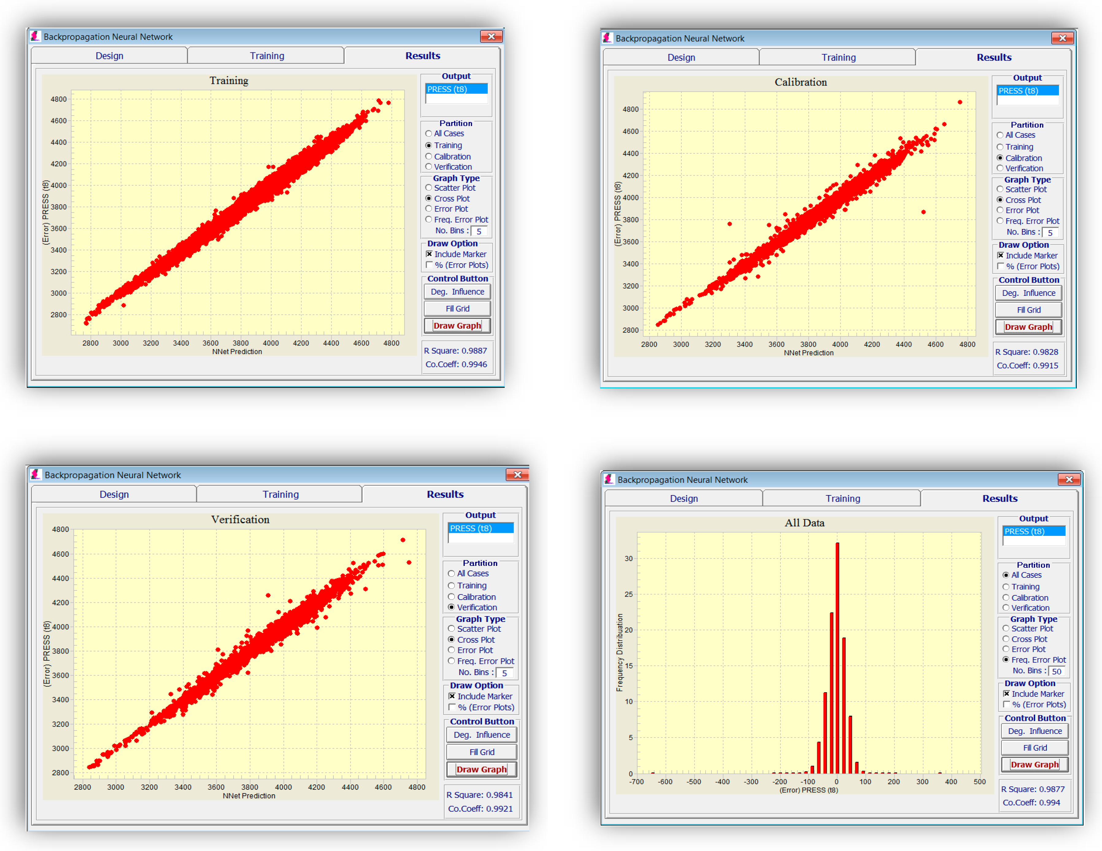
Different parameters, such as momentum and learning rate, can be changed in an attempt to train a better network. The results of network training for pressure at 1 January 2009 are demonstrated in
Figure 6. The frequency of error can be plotted to analyze and verify the accuracy of the network.
The stoppage criterion in all the networks is reaching the best calibration set to prevent an over-fitting problem. R-squared can be used as a relative yardstick for verifying the model integrity while training and determining how well it might predict the results of a new dataset.
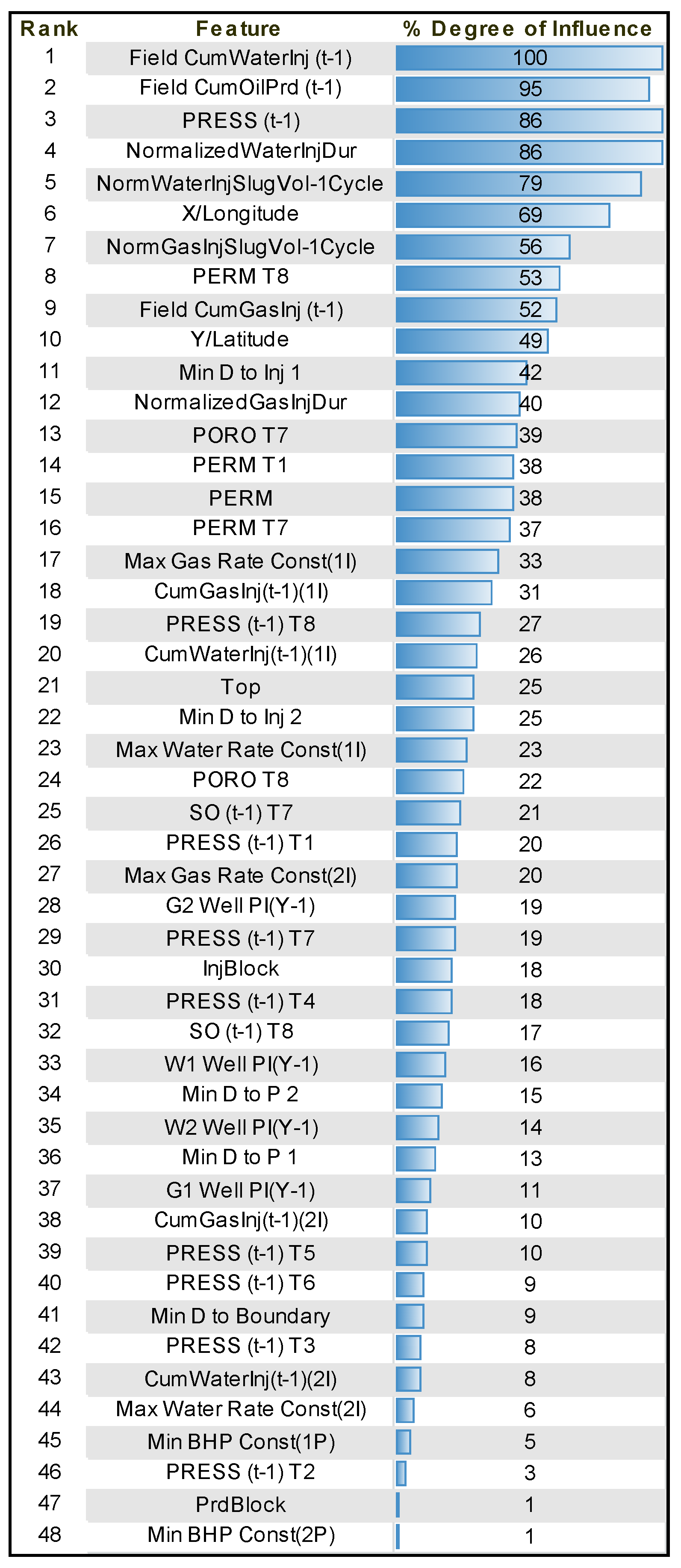
Upon completion of training, the parameters that have had the most weight in the training process can be listed alongside their relative influence percentage. These parameters for pressure at 1 January 2009 are listed in
Figure 7. As can be seen, volumetric changes in the field in terms of injected and produced fluid, injection scheme properties, and pressure in the last time step have the highest importance among the dynamic properties. Permeability and porosity are the most influential static parameters.
2.3.2. Well-Based SRM (SRMW)
Well-based SRMs are used when the objective is to simulate the response of the reservoir at well level (rate) to different reservoir parameters or operational constraints. Since the run time of a well-based SRM is much smaller than the traditional reservoir models, it becomes extremely useful in engineering tasks requiring many simulation runs, such as sensitivity analysis, uncertainty quantification, history matching, and optimization, which all are a part of master development plans or asset-level decision making.
Since the objective of this study is to build the basis of optimization, building a well-based SRM is important. Using the well-based SRM, the best injection scenario can be decided upon. This decision is based on the amount of oil production from each well with respect to changes in operational constraints. The CO2 utilization factor, which is the ratio of CO2 used to the volume of oil produced, is a common factor for comparing different scenarios in an optimization course.
As explained before, the development of a spatio-temporal database is the first step in building SRM.
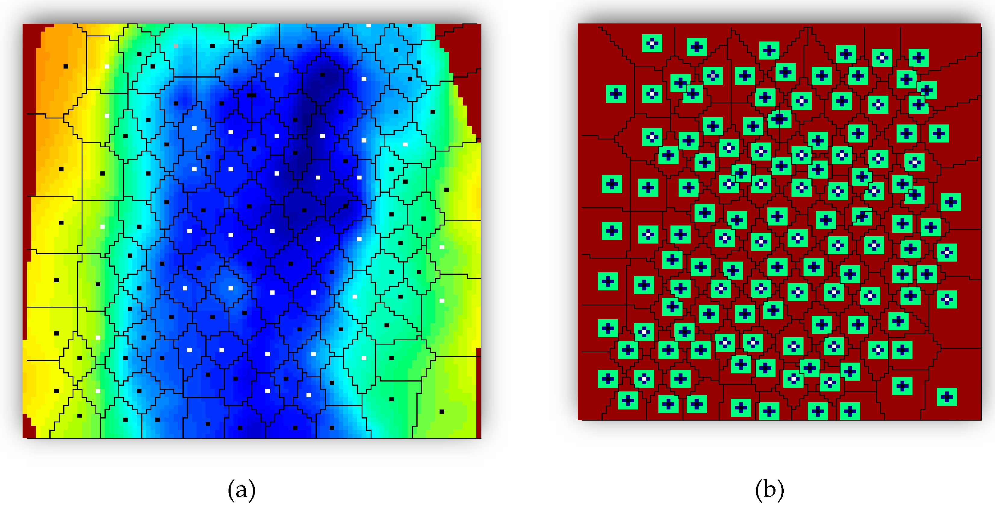
Table 5 shows the main properties that should be considered for building the well based database. Volumetric analyses data can be used for expressing more statistics of the reservoir. To do so, reservoir delineation and tiering were performed. Reservoir delineation provided a uniform spatial distributed pattern based on the Voronoi graph theory [
34]. It is assumed that each well is contributing to production based on its assigned drainage area and relative reservoir characteristics. Polygon (Voronoi) based information can also be encompassed in the final dataset, which carries a higher information content in comparison with values at each specific well block. Three tiers were defined based on the proximity of the gridblocks to each well.
As most of the dynamic changes take place around the wells, it is important to keep the resolution in this area. Thereby, a specific number of gridblocks were assigned to tier 1 and tier 2 based on their distance to each well. Tier values were calculated for each property at each layer. Since the model is heterogeneous in terms of structure, a weighted value was calculated for the final tier corresponding to each well-based on the single layer properties. After determining tier 1 and 2, the remaining gridblocks in each well polygon (Voronoi cell) were used to calculate tier 3 for the corresponding well (
Figure 8 and
Figure 9).
The same procedure described in the grid-based SRM development was followed. Upon data base generation, statistical and key performance indicator (KPI) analysis was performed to pick the most influential properties.
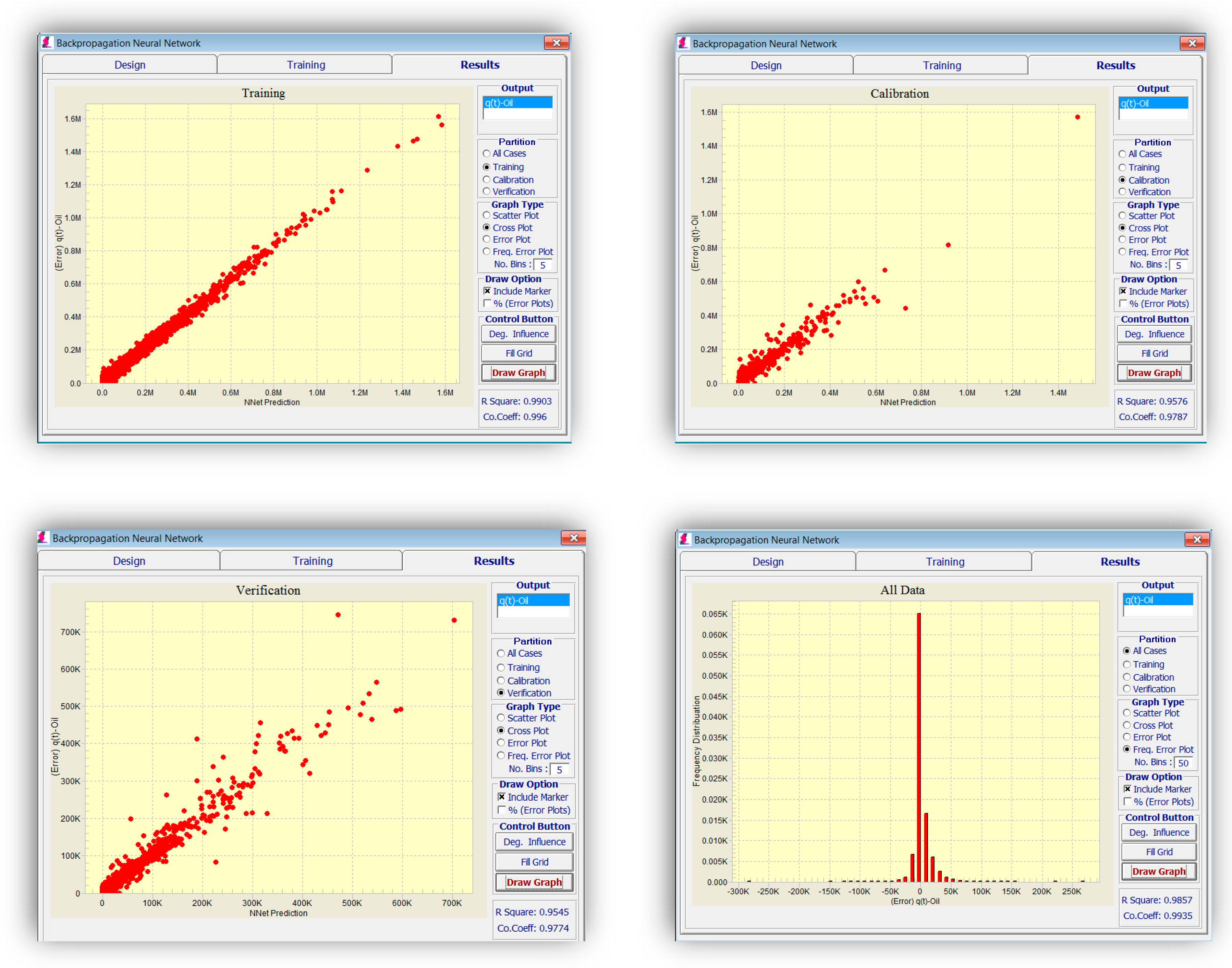
Table 6 displays a sample list of the inputs used for modeling oil production. The data was partitioned randomly to assign 80% to the training set, and 10% to each of the calibration and validation sets. Three different networks were designed for oil, water, and CO
2 production, each of them having three layers (input, hidden, and output layers). The backpropagation algorithm was used for training the network. In general, the network architecture is not a crucial factor in making it a success or failure. On the contrary, the type of inputs can have a substantial effect on the results.
Figure 10 shows the training results for oil production. As explained above, 80% of the data was used for training, 10% for calibration, and the rest for validation. The criteria for stoppage was set to be the best calibration result. This means, in case the error of the training set is still decreasing with each epoch, while the error of the calibration set is increasing, the training would stop to prevent “memorizing” or “over-fitting” of the network and guarantee its generalization capability. As seen in
Figure 10, the error is comparatively low in all training, calibration, and validation sets (which was not used for training).
As explained in the SRMG section, the coefficient of determination, denoted by R
2, is used for indicating how well data is represented by the built model. This coefficient is listed for the oil, water, and gas production models shown in
Table 7.
2.3.3. Coupled SRM
The process of coupling the grid-based and well-based SRM was implemented in this work for the first time. In an optimization process, the flood front monitoring is as important as the production rate estimation.
To this end, we propose to assimilate the SRMG and SRMW by feeding the data from one model to another one. The coupled SRM will be a great tool in accomplishing the following tasks:
Monitoring the interaction of wells with one another.
Monitoring flood front during water flood or gas injection operations.
Optimizing injection rates for maximum sweep efficiency.
New well placements to optimize enhanced recovery.
Developing new strategies for field development.
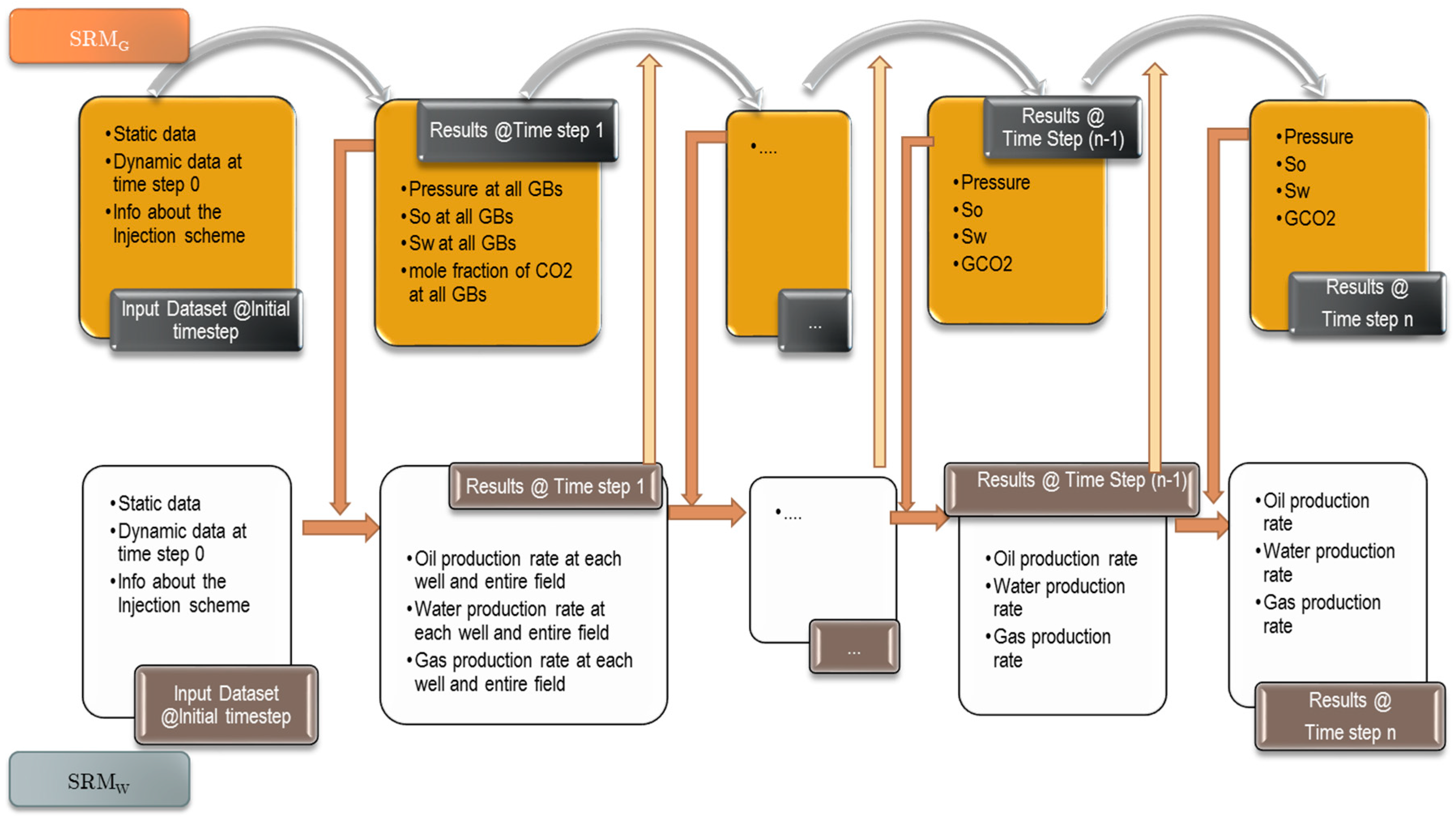
Figure 11 shows the flowchart of performing coupled surrogated reservoir modeling. Two distinct databases are used for the integration course. The grid-based spatio-temporal database encompasses the static and dynamic data at the initial time step before the injection scheme initiates. This part of the dataset is unique no matter what injection scheme is in play. The only data required apart from this common database is the information about the injection scheme and operational constraints based on the desired WAG ratio. The same holds for the well-based spatio-temporal dataset.
The process starts with the grid-based database. Upon running the SRMG, the pressure, phase saturation, and CO2 mole fraction are calculated for all the gridblocks in the model for the succeeding time step. This information is processed, well productivity index (PI) calculation and tiering computations pertaining to grid-based and well-based systems are performed. The calculated values accompanied by the well-based initial information are fed to the SRMW. Implementing this model will yield the oil, water, and CO2 production of the wells and the entire field at the first time-step. Accordingly, the cumulative values in the wells and the entire field, in consort with the water cut and gas oil ratio, in each well is calculated. The database which is going to be used for the SRMG and SRMW in the next step is updated correspondingly, and the SRMG is run again to produce the dynamic data of the subsequent time step. The sequence is continued until the last time step (year) is reached.
3. Results
A total of 60 neural network models was combined to create an ensemble forming the SRMG for each individual property (15 models per property). The SRM uses a cascading feature. With an initial dataset, including the reservoir dataset at the beginning, the trained models at each year are used to predict the output at each time step. The output of the model at each time step encompasses the pressure, oil saturation, water saturation, and the global mole fraction of CO2 at each gridblock of the reservoir. The output of each individual model along with the calculated tier values is imported into the database of the next time. This process continues until the last year is reached. The total time taken for deploying the SRM and performing the cascading calculations using 60 networks is almost 800 s.
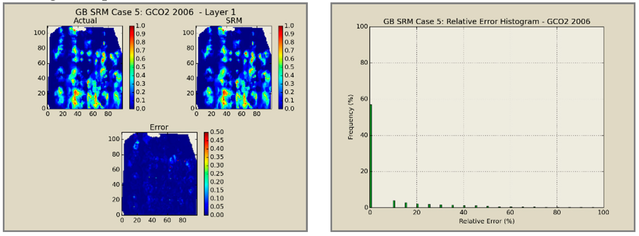
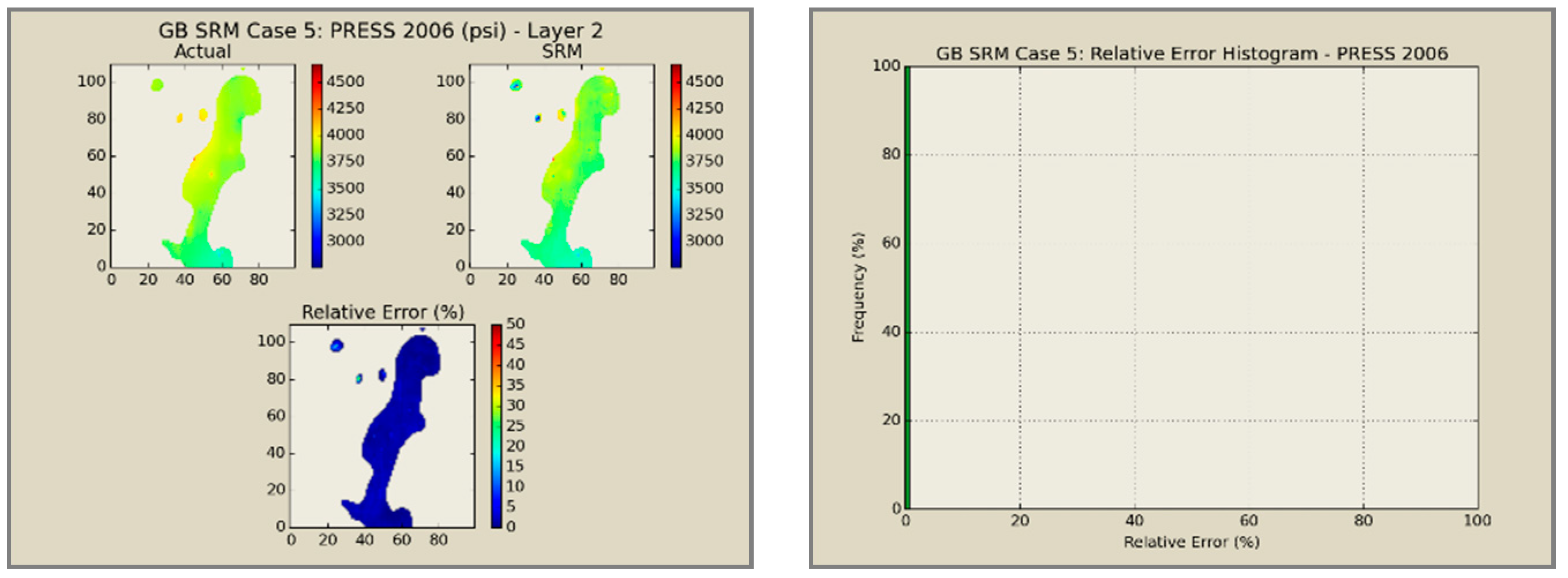
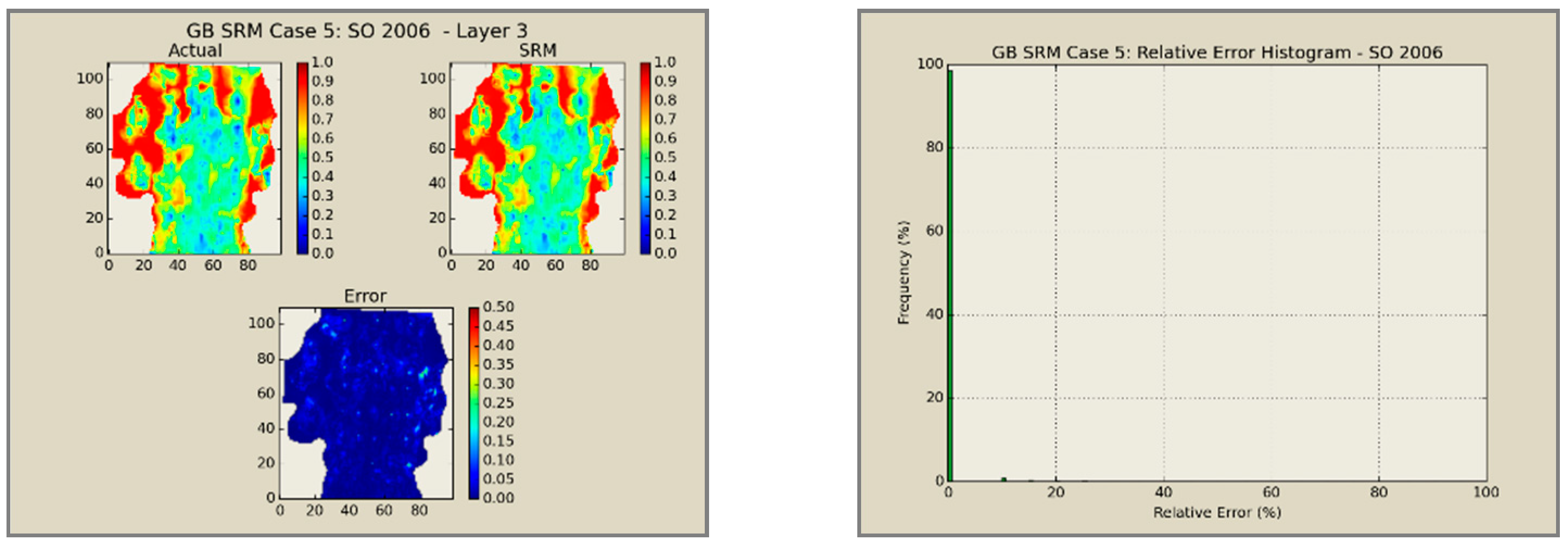
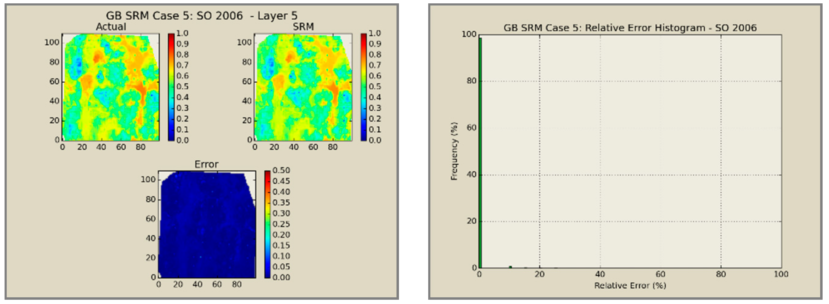
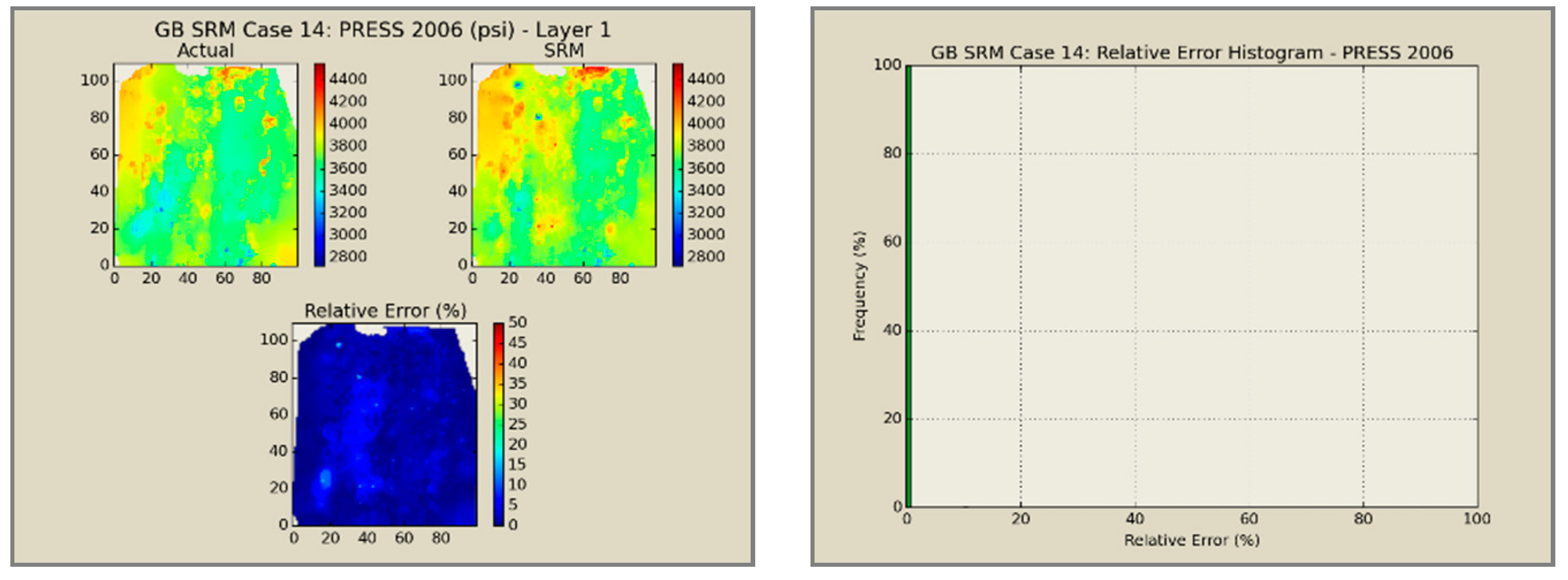
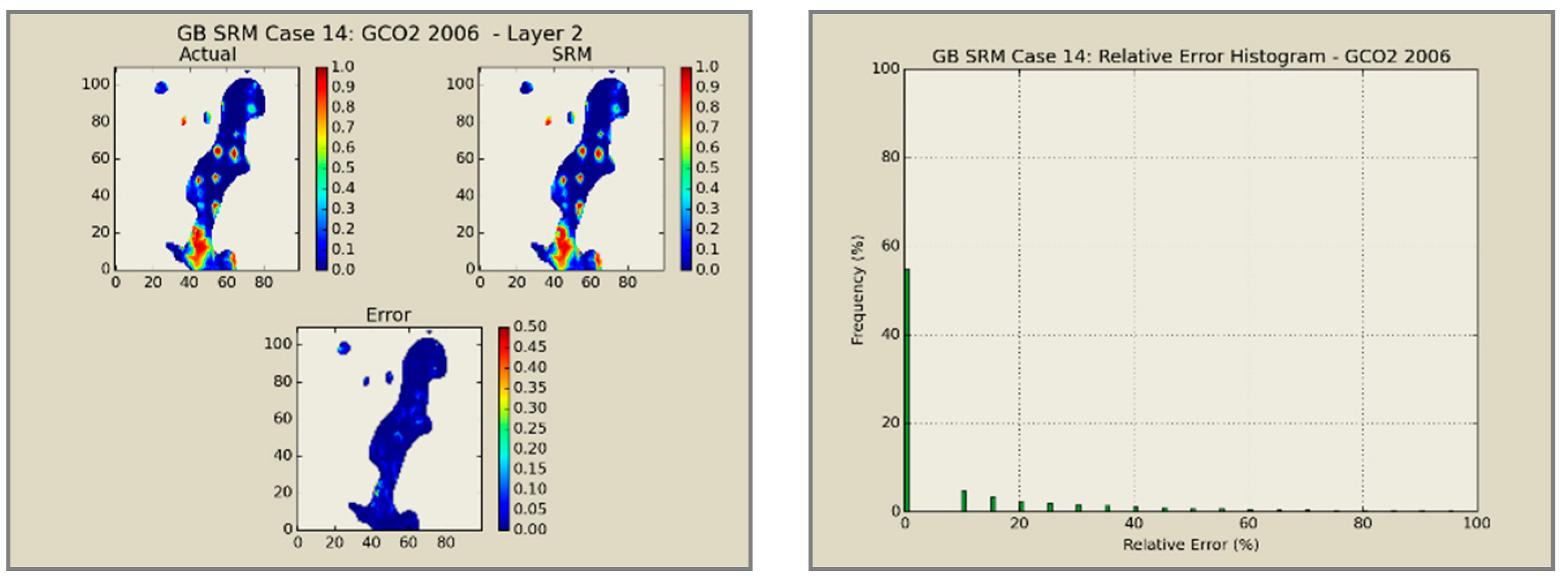
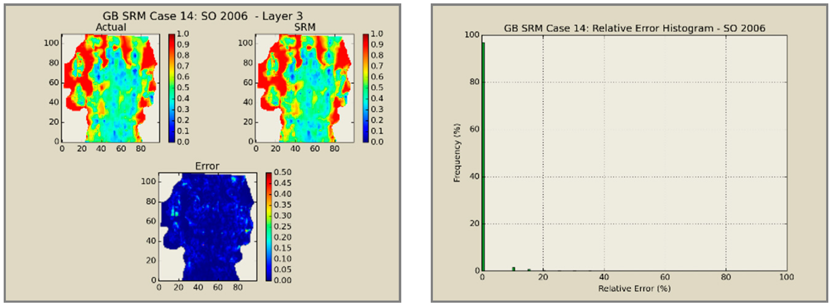
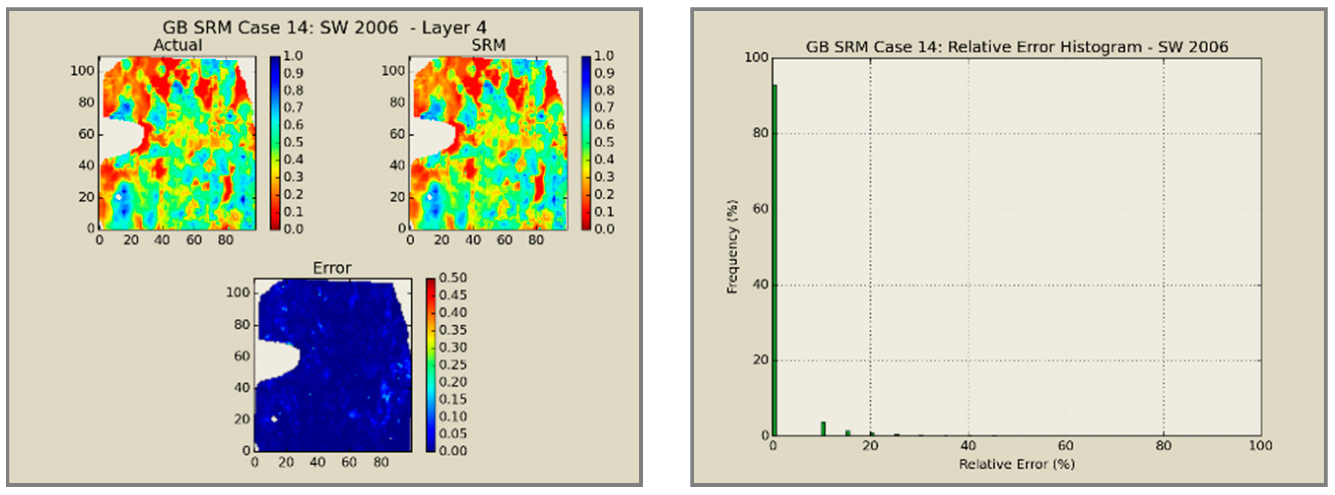
Figure 12,
Figure 13,
Figure 14 and
Figure 15 presents the results of the coupled SRM in terms of pressure, phase saturation, and component mole fraction accompanied by an error histogram, for one of the cases (scenario 5) after the first cycle of WAG as an example. For simplicity purposes, only one of the reservoir layers is shown for each of the dynamic variables. The uncolored area is outside the reservoir boundary, or represents the area that the formation is pinched. A comprehensive set of figures that compares all the results from the smart proxy and the numerical reservoir simulation model can be found in the reference document mentioned in this article [
31]. The error has been shown, proving the high accuracy of the SRM. It should be noted that the network was trained with only 6% of the data and 94% of each case is totally blind and was not used in any part of the training process.
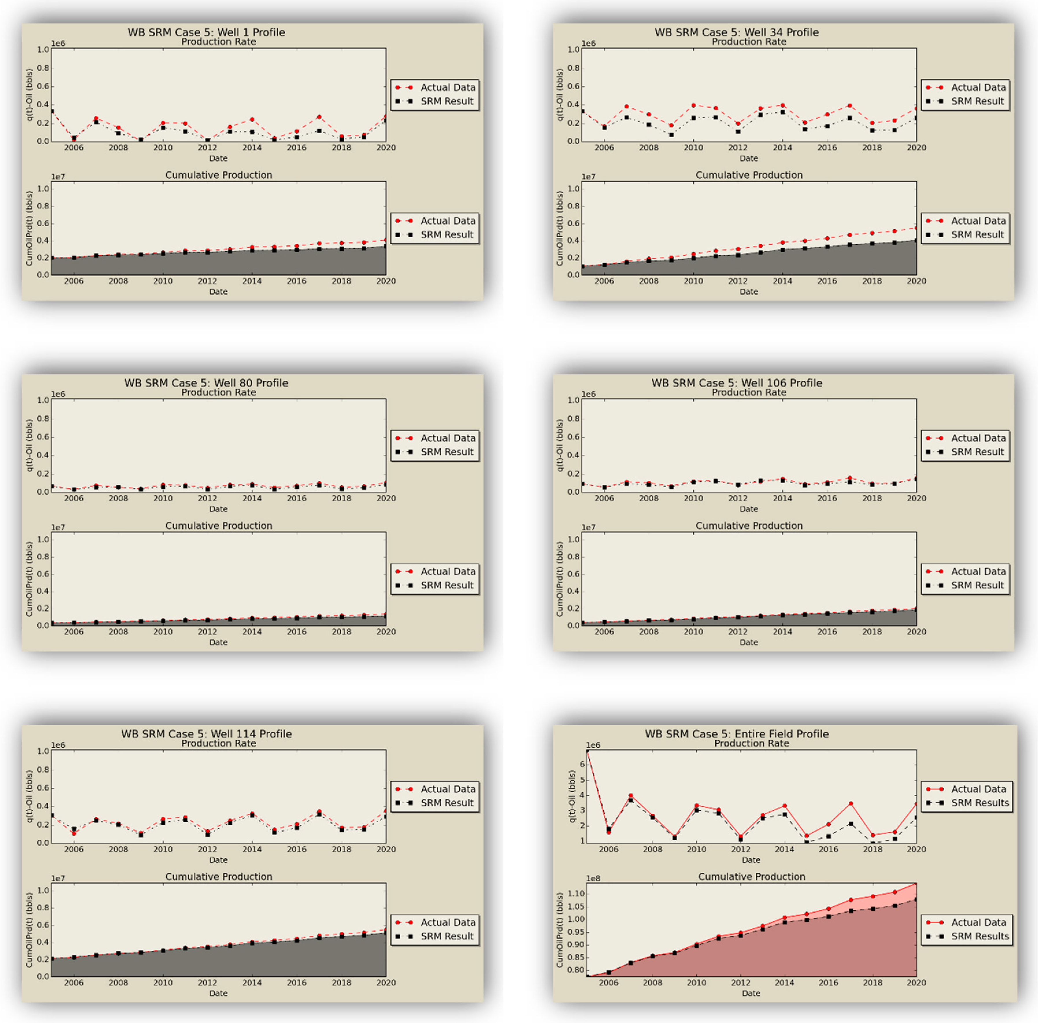
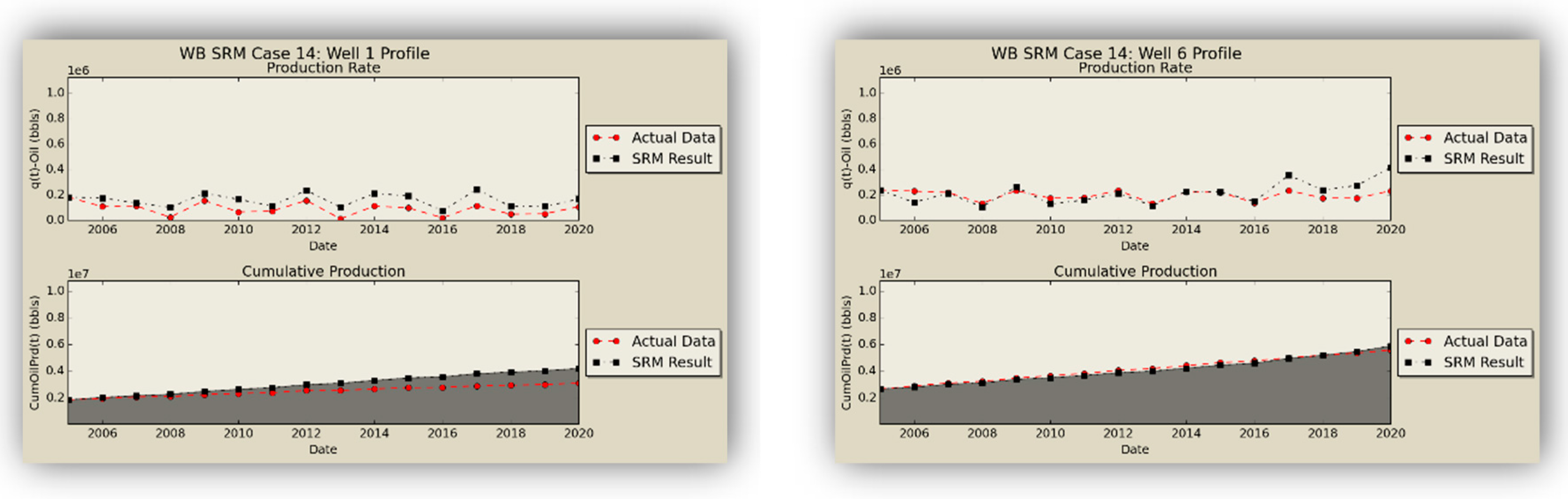
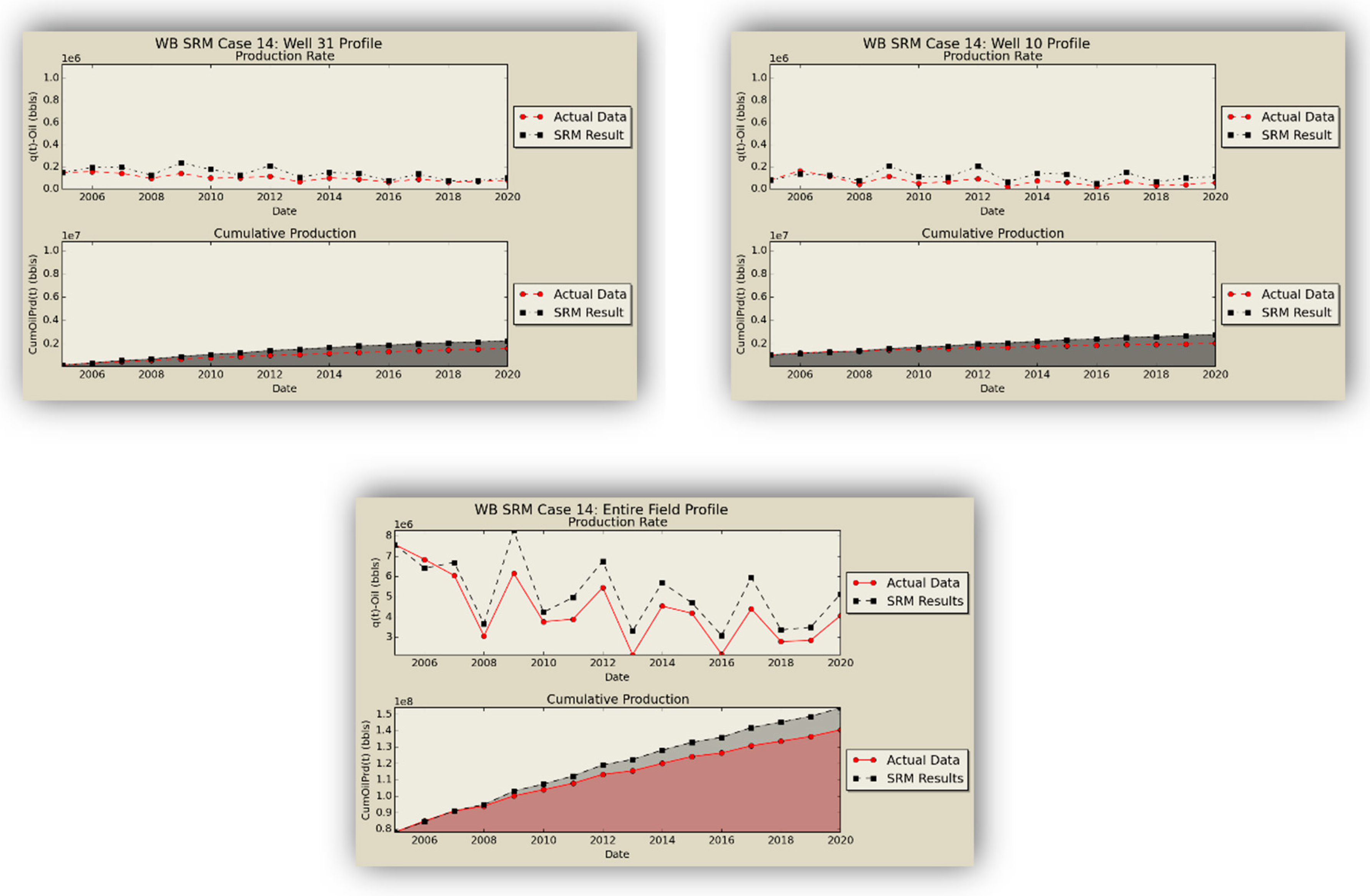
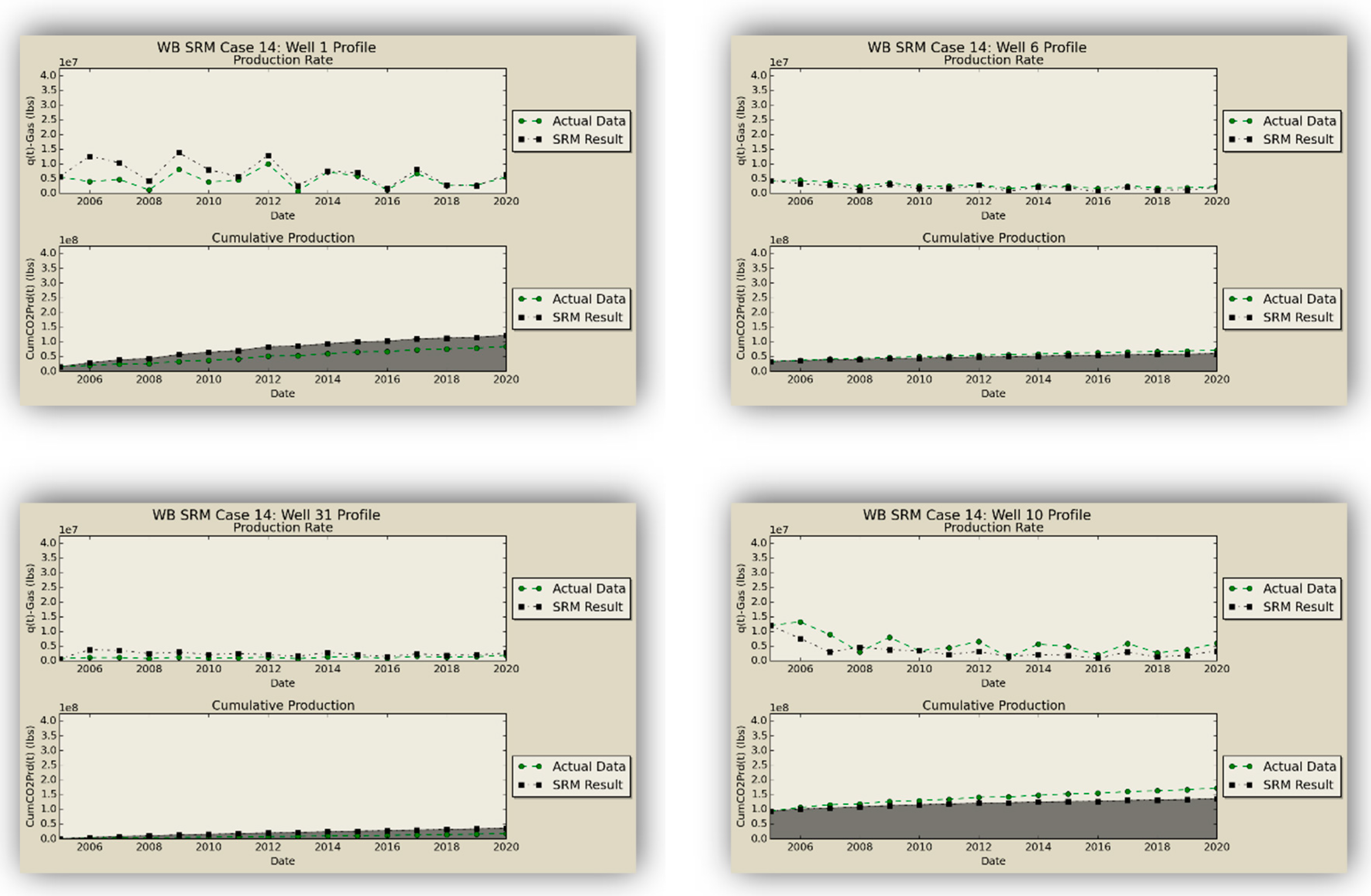
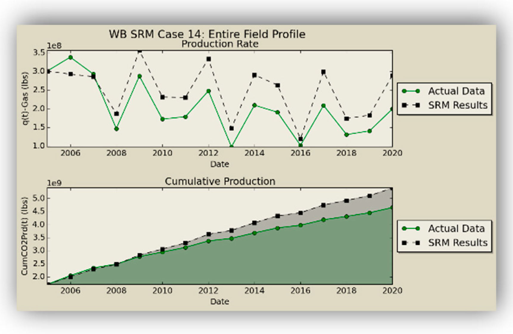
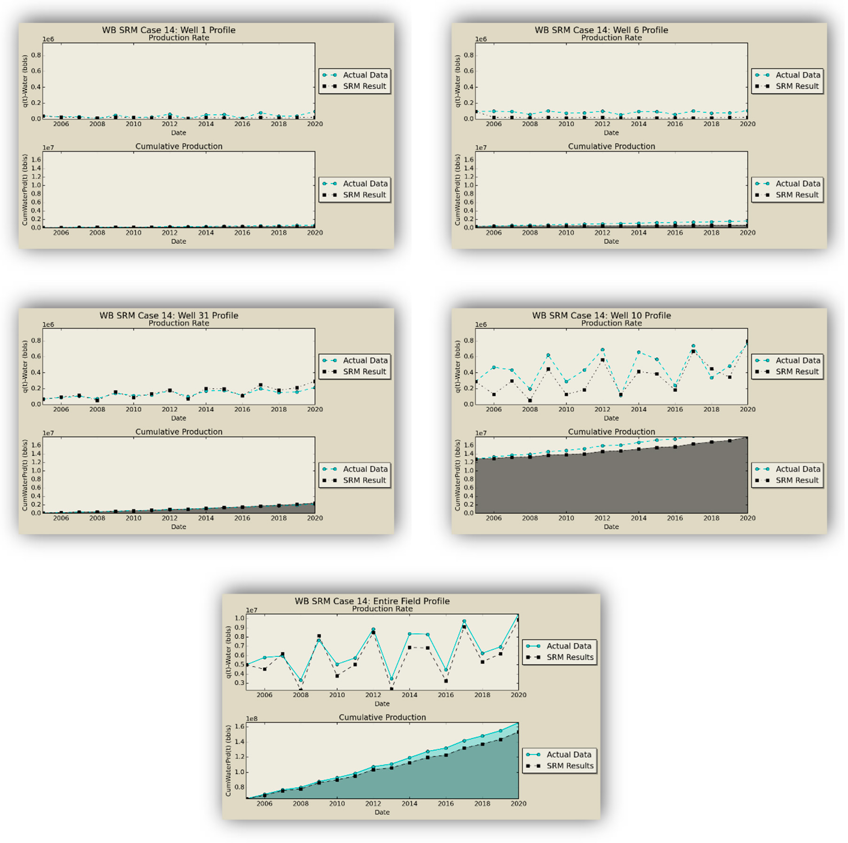
After the networks were studied in a standalone fashion to determine their individual quality, they were applied in a cascading feed-forward design in order to obtain a fully-fledged well-based surrogate model (SRM
W) as the replica of the former numerical reservoir model. The oil production rates obtained from the coupled SRM are demonstrated in
Figure 16.
SRM does an excellent job in qualitative representation of the fronts and presents acceptable results in predicting the quantities.
The robustness of the model was tested via different experiments. First, a part of the dataset was set aside (validation partition) while training the neural network and was later used for testing the integrity of the created neural network. The network showed high accuracy in the validation part. This was ensured by deploying the built SRM on different scenarios. Although part of the data was used in building the model, 94% of the records was not used in any part of the model generation. As shown in this section, the accuracy of the model was approved in this test as well. Apart from this test, it was decided to build a new scenario based on a totally new injection scheme and operational constraints. This information is not included in any part of the spatio-temporal database used for SRM development and is called the “blind set”.
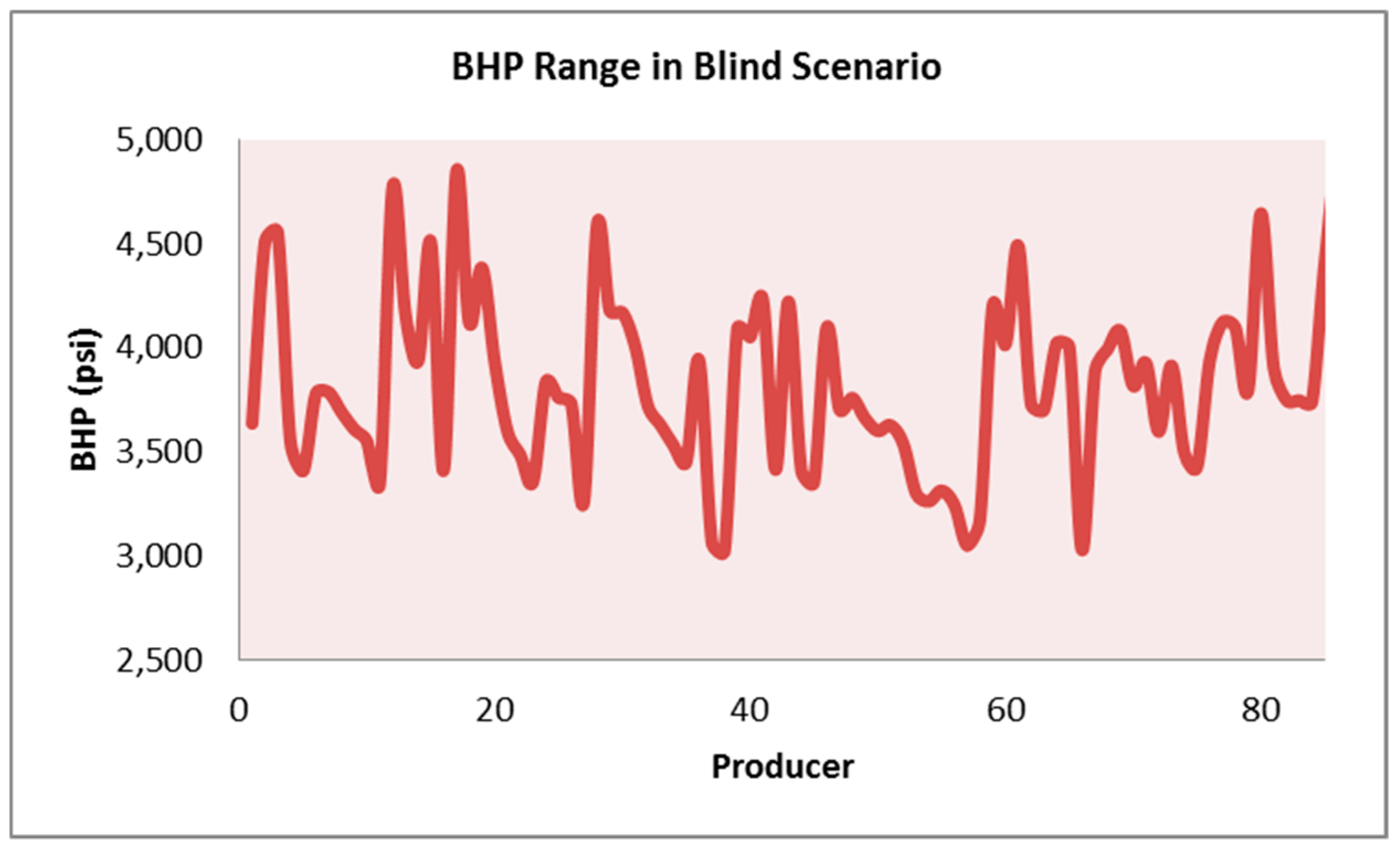
Figure 17,
Figure 18, and
Table 8 show the injection schematic and operational constraints, along with the results of the blind test, illustrating the high accuracy of the SRM predictions.
The grid-based results are visualized in
Figure 19,
Figure 20,
Figure 21 and
Figure 22, and the oil, gas, and water production results from the numerical simulation and SRM prediction on the blind case are compared in
Figure 23,
Figure 24 and
Figure 25 and prove the applicability of the coupled SRM. As explained before, one property per layer is shown for simplicity. While there is close proximity between the trained scenarios and SRM results, there is a difference in some cases of the blind set. This is mostly due to the fact that none of the parameters of the blind case (static or dynamic properties) were used in the trained model, also the error was propagated because the results of one time-step cascades to another.
4. Discussion
Although many techniques have been made available for production optimization in the upstream oil and gas industry, it is still a challenging task to optimize reservoir performance in the presence of physical and/or financial uncertainties [
35]. Economic success of an EOR project principally depends on the efficiency of the selected method in the reservoir of interest and the way it is deployed. Owing to the heavy computational work that is compulsory for a large number of simulations, it is rather a laborious and tedious task to determine optimum design schemes for a given project.
Proxy modeling has been introduced as an alternative to traditional reservoir modeling for conducting a high number of runs in the petroleum industry in recent years, although there has been a resistance toward shifting from traditional reservoir modeling to proxy modeling. One of the most important reasons for this defiance is getting used to traditional reservoir modeling. As Mark Twain says “Nothing so needs reforming as other people’s habits.” Bad presentation of the proxy models and their application is another reason for making this paradigm shift even harder. It should be specified when the proxy models are of the best use and under what circumstances they can be used in conjunction with numerical reservoir simulation tools or independent from them.
The procedure for building a surrogate reservoir model (SRM) was explained in detail through the course of this work. This study was performed to provide a base for optimization by investigating the feasibility of using state-of-the-art data-driven proxy models through development of a surrogate reservoir model in the SACROC field with more than 30 years of CO2-EOR.
The intricacy of simulating multiphase flow, especially in the case of miscible CO2 injection, with many time steps required the reservoir response to the injection to be studied, with the highly heterogonous reservoir and numerous number of wells all contributing to the complexity of the problem. The necessity of the SRM has to do with the fact that the massive potential of the existing numerical reservoir simulation models goes unrealized, attributable to the long time required to make a single run. Even on a cluster of parallel CPUs, numerical models that are built to simulate complex reservoirs with multi-million gridblocks entail substantial run-time.
The simulation time for a single run of the built model for the total life of the reservoir took almost a month. Using design of experiment techniques, multiple WAG scenarios were planned, and corresponding models were created and run. The spatio-temporal database was created based on the generated data. Data mining and artificial intelligence techniques were employed for devising two different types of surrogate reservoir models, with the ability of estimating the potential of wells in terms of production and dynamic distribution of different properties in every single gridblock of the reservoir. These models were coupled to provide an integrated SRM, which can predict the reservoir dynamic response both at the well and grid level.
In some cases, it might seem the grid-based model generates better results than the well-based. This can be explained by the fact that the number of representative samples in the database records plays a very important role. As seen in the grid-based model, the network had a better prediction for grids that has more representative or similar samples in the spatio-temporal database, because it had learned their behavior better. In the well-based models, the samples and consequently the data records are less compared to gridblocks.
By defining an objective function (e.g., net present value or CO2 utilization factor), the coupled SRM can be used to run and compare hundreds of scenarios based on various injection schemes and WAG ratios and determine the optimal scenario using an optimization algorithm.
It takes more than 48 h for one run (the life span used for optimization design) to be completed using a commercial reservoir simulator on a machine with 24 GB RAM and a 3.47 GHz processor. The run time of each model in the SRM on the same machine is 15 s out of which 10 s pertains to the SRM deployment at each step. If 100 runs are required for performing an optimization process, it will take almost 7 months to carry out all the runs; this duration increases up to almost 6 years for 1000 runs, making the whole procedure impractical and unattainable. Using the SRM, on the other hand, will only take a bit more than a day or less than two weeks to perform 100 or 1000 runs correspondingly, which is a huge accomplishment.
Coupled SRM was developed in this study for the first time. At the time of this study, none of the works conducted on this topic had ever been performed at this scale of complexity neither at the well-based nor grid-based level. Similar works at the well-based level have been done on the order of a maximum of 10 wells. Moreover, the main focus has never been on grid-based values and they have been used only as a means for rate calculation. The grid-based prediction has been performed typically in 2-D and two-phase reservoirs. This highlights the achievements of this study, which were performed on a compositional heterogeneous high order 3-D, 3-phase reservoir model with 3,622,190 geocellular blocks (396,000 gridblocks), 40 injection, and 75 production wells and undergoing a miscible CO2-EOR process.


