Three-Dimensional Simulation of Fluid–Structure Interaction Problems Using Monolithic Semi-Implicit Algorithm

Abstract

A monolithic semi-implicit method is presented for three-dimensional simulation of fluid–structure interaction problems. The updated Lagrangian framework is used for the structure modeled by linear elasticity equation and, for the fluid governed by the Navier–Stokes equations, we employ the Arbitrary Lagrangian Eulerian method. We use a global mesh for the fluid–structure domain where the fluid–structure interface is an interior boundary. The continuity of velocity at the interface is automatically satisfied by using globally continuous finite element for the velocity in the fluid–structure mesh. The method is fast because we solve only a linear system at each time step. Three-dimensional numerical tests are presented.

1. Introduction

There exists a rich literature on solving numerically fluid–structure interaction problems. Some methods are based on partitioned procedures, the fluid and structure sub-problems are solved separately using iterative process: fixed point iterations [1,2,3], Newton-like methods [4,5,6] or optimization techniques [7,8,9]. Monolithic methods solve the fluid–structure interaction problem as a single system of equations, [10,11,12,13], or more recently [14,15,16,17].

In some methods such as the Arbitrary Lagrangian Eulerian (ALE) framework, the fluid equations are written over a moving mesh which follows the structure displacement (see [18,19]). Other methods use a fixed mesh for fluid domain: immersed boundary method [20], distributed Lagrange multiplier [21,22], penalization [23,24], extended finite element method (XFEM) [25,26], and Nitsche-XFEM [27]. Distributed Lagrange multiplier strategy with remeshing is used in [28] and a monolithic fictitious domain without Lagrange multiplier is employed in [29,30].

Most of these methods are implicit. For a long time, the explicit methods were considered not suitable because of the lack of stability, but these methods are successfully applied in [31,32]. A third class of methods are so-called semi-implicit methods, where the domain is computed explicitly while the fluid velocity and pressure as well as the structure displacement are computed implicitly, [33,34]. In [35], it is proved that a schema of this kind is unconditionally stable.

In this paper, a monolithic semi-implicit method is employed for three-dimensional simulation. For the structure modeled by the linear elasticity equations, we use the updated Lagrangian framework and, for the fluid governed by the Navier–Stokes equations, we employ the ALE method. A similar strategy is used in [36] for a bi-dimensional compressible neo-Hookean model or in [37] for a bi-dimensional linear elasticity model for the structure. As in [38], we employ a global mesh for the fluid–structure domain where the fluid–structure interface is an interior boundary. Using globally continuous finite element for the velocity in the fluid–structure mesh, the continuity of velocity at the interface is automatically satisfied. The method is fast because we solve only a linear system at each time step. Three-dimensional numerical tests are presented.

In [14,15,16,17], a global mesh obtained from the deformed structure mesh and a fluid mesh generated at each time step, compatible at the interface with the structure mesh are used. Remeshing the fluid domain improves the quality of the mesh in the case of large deformation. The non-linear structure equation written in the Eulerian coordinates is obtained by using Cayley–Hamilton theorem. The fluid equations are solved by the characteristics method. The weak formulation of the fluid–structure interaction problem is written in the Eulerian domain, which is unknown, and a fixed-point algorithm solves the global non-linear problem at each time step.

In [30], it is assumed that the structure is viscoelastic with the same viscosity as the fluid. Based on fictitious domain without Lagrange multiplier, the fluid is solved in a fixed mesh of the fluid–structure domain. The weak formulation contains integrals over the unknown Eulerian domain of the structure. At each time step, a fixed-point algorithm is employed.

In [36], by using the Updated Lagrangian framework for a compressible Neo-Hookean structure, the weak formulation is written in the known configuration obtained at the precedent time step. By linearization around this configuration, at each time step, only a linear system is solved for the fluid–structure coupled equations and consequently the computing time is reduced. In the present paper, we follow this approach for three-dimensional simulations using linear elastic model for the structure.

If at each time step of the monolithic implicit methods, the fixed-point algorithm does not converge quickly or the computational time by fixed-point iteration is very expensive, thus the monolithic semi-implicit methods, which have similar stability properties and a reduced computational time, could be a good alternative.

2. Problem Statement

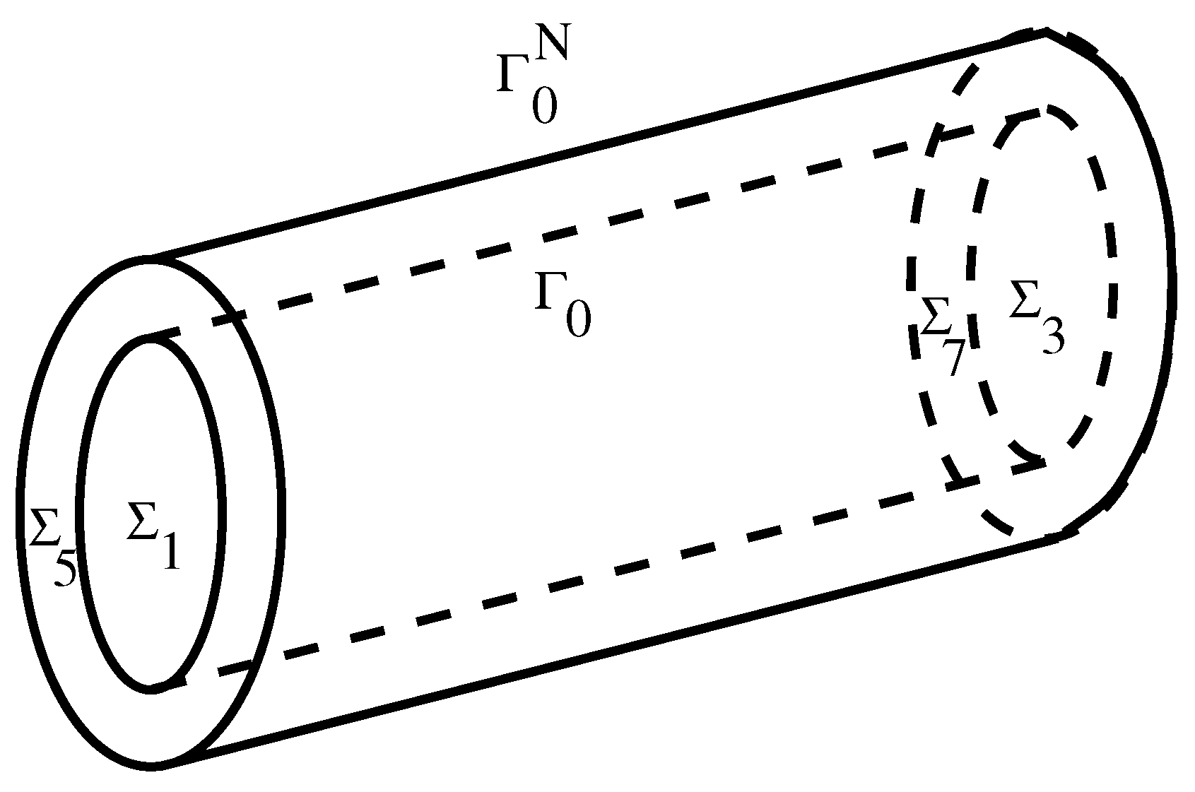
The initial fluid domain ${\Omega }_0^F$ is a right circular cylinder of bases ${\Sigma }_1$, ${\Sigma }_3$ and lateral surface ${\Gamma }_0$. We denote by ${\Omega }_0^S$ the initial structure domain and we assume that it is a right annular cylinder of bases ${\Sigma }_5$, ${\Sigma }_7$, interior lateral surface ${\Gamma }_0$ and exterior lateral surface ${\Gamma }_0^N$ (see Figure 1). We suppose that the initial structure domain is undeformed (stress-free). The boundary ${\Gamma }_0$ is common of both domains and it represents the initial position of the fluid–structure interface.

At the time instant t, the fluid occupies the domain ${\Omega }_t^F$ bounded by the moving interface ${\Gamma }_t$ and by the fixed boundaries ${\Sigma }_1$, ${\Sigma }_3$, while the structure occupies the domain ${\Omega }_t^S$ bounded by the moving lateral surfaces ${\Gamma }_t$, ${\Gamma }_t^N$ and by the fixed boundaries ${\Sigma }_5$, ${\Sigma }_7$.

We denote by ${\mathbf{U}}^S:{\Omega }_0^S\times \left[0,T\right]\to {\mathbb{R}}^3$ the displacement of the structure. A particle of the structure whose initial position was the point $\mathbf{X}$ will occupy the position $\mathbf{x}=\mathbf{X}+{\mathbf{U}}^S\left(\mathbf{X},t\right)$ in the deformed domain ${\Omega }_t^S$. At the time instant t, the interface ${\Gamma }_t$ is the image of ${\Gamma }_0$ via the map $\mathbf{X}\to \mathbf{X}+{\mathbf{U}}^S\left(\mathbf{X},t\right)$. The same relationship exists between ${\Gamma }_t^N$ and ${\Gamma }_0^N$. On ${\Gamma }_0^D={\Sigma }_5\cup {\Sigma }_7$, we impose zero displacements.

We set ${\nabla }_{\mathbf{X}}{\mathbf{U}}^S$ the gradient of the displacement ${\mathbf{U}}^S={\left(U_1^S,U_2^S,U_3^S\right)}^T$ with respect to the Lagrangian coordinates $\mathbf{X}={\left(X_1,X_2,X_3\right)}^T$. We denote by $\mathbf{F}\left(\mathbf{X},t\right)=\mathbf{I}+{\nabla }_{\mathbf{X}}{\mathbf{U}}^S\left(\mathbf{X},t\right)$ the gradient of the deformation, where $\mathbf{I}$ is the unity matrix and we set $J\left(\mathbf{X},t\right)=\det \mathbf{F}\left(\mathbf{X},t\right)$. The second Piola–Kirchhoff stress tensor is denoted by $\Sigma$.

We assume that the fluid is governed by the Navier–Stokes equations. For each time instant $t\in [0,T]$, we denote the fluid velocity by ${\mathbf{v}}^F\left(t\right)={\left(v_1^F\left(t\right),v_2^F\left(t\right),v_3^F\left(t\right)\right)}^T:{\Omega }_t^F\to {\mathbb{R}}^3$ and the fluid pressure by $p^F\left(t\right):{\Omega }_t^F\to \mathbb{R}$. Let $ϵ\left({\mathbf{v}}^F\right)=\frac{1}{2}\left(\nabla {\mathbf{v}}^F+{\left(\nabla {\mathbf{v}}^F\right)}^T\right)$ be the fluid rate of strain tensor and let ${\sigma }^F=-p^F\mathbf{I}+2{\mu }^Sϵ\left({\mathbf{v}}^F\right)$ be the fluid stress tensor. To simplify the notation, we write $\nabla {\mathbf{v}}^F$ in place of ${\nabla }_{\mathbf{x}}{\mathbf{v}}^F$, when the gradients are computed with respect to the Eulerian coordinates $\mathbf{x}$.

The problem is to find the structure displacement ${\mathbf{U}}^S$, the fluid velocity ${\mathbf{v}}^F$ and the fluid pressure $p^F$ such that:

$$\begin{array}{lll}{\rho }_0^S\left(\mathbf{X}\right)\frac{{\partial }^2{\mathbf{U}}^S}{\partial t^2}\left(\mathbf{X},t\right)-{\nabla }_{\mathbf{X}}·\left(\mathbf{F}\Sigma \right)\left(\mathbf{X},t\right)& =& {\rho }_0^S\left(\mathbf{X}\right)\mathbf{g},\mathrm{in}{\Omega }_0^S\times (0,T)\end{array}$$

(1)

$$\begin{array}{lll}{\mathbf{U}}^S\left(\mathbf{X},t\right)& =& 0,\mathrm{on}{\Gamma }_0^D\times (0,T)\end{array}$$

(2)

$$\begin{array}{lll}\left(\mathbf{F}\Sigma \right)\left(\mathbf{X},t\right){\mathbf{N}}^S\left(\mathbf{X}\right)& =& 0,\mathrm{on}{\Gamma }_0^N\times (0,T)\end{array}$$

(3)

$$\begin{array}{lll}{\rho }^F\left(\frac{\partial {\mathbf{v}}^F}{\partial t}+({\mathbf{v}}^F·\nabla ){\mathbf{v}}^F\right)-2{\mu }^F\nabla ·ϵ\left({\mathbf{v}}^F\right)+\nabla p^F& =& {\rho }^F\mathbf{g},\forall t\in (0,T),\forall \mathbf{x}\in {\Omega }_t^F\end{array}$$

(4)

$$\begin{array}{lll}\nabla ·{\mathbf{v}}^F& =& 0,\forall t\in (0,T),\forall \mathbf{x}\in {\Omega }_t^F\end{array}$$

(5)

$$\begin{array}{lll}{\sigma }^F{\mathbf{n}}^F& =& {\mathbf{h}}_{in},\mathrm{on}{\Sigma }_1\times (0,T)\end{array}$$

(6)

$$\begin{array}{lll}{\sigma }^F{\mathbf{n}}^F& =& {\mathbf{h}}_{out},\mathrm{on}{\Sigma }_3\times (0,T)\end{array}$$

(7)

$$\begin{array}{lll}{\mathbf{v}}^F\left(\mathbf{X}+{\mathbf{U}}^S\left(\mathbf{X},t\right),t\right)& =& \frac{\partial {\mathbf{U}}^S}{\partial t}\left(\mathbf{X},t\right),\mathrm{on}{\Gamma }_0\times (0,T)\end{array}$$

(8)

$$\begin{array}{lll}{\left({\sigma }^F{\mathbf{n}}^F\right)}_{\left(\mathbf{X}+{\mathbf{U}}^S\left(\mathbf{X},t\right),t\right)}& =& -\left(\mathbf{F}\Sigma \right)\left(\mathbf{X},t\right){\mathbf{N}}^S\left(\mathbf{X}\right),\mathrm{on}{\Gamma }_0\times (0,T)\end{array}$$

(9)

$$\begin{array}{lll}{\mathbf{U}}^S\left(\mathbf{X},0\right)& =& {\mathbf{U}}^{S,0}\left(\mathbf{X}\right),\mathrm{in}{\Omega }_0^S\end{array}$$

(10)

$$\begin{array}{lll}\frac{\partial {\mathbf{U}}^S}{\partial t}\left(\mathbf{X},0\right)& =& {\mathbf{V}}^{S,0}\left(\mathbf{X}\right),\mathrm{in}{\Omega }_0^S\end{array}$$

(11)

$$\begin{array}{lll}{\mathbf{v}}^F\left(\mathbf{X},0\right)& =& {\mathbf{v}}^{F,0}\left(\mathbf{X}\right),\mathrm{in}{\Omega }_0^F\end{array}$$

(12)

where ${\rho }_0^S:{\Omega }_0^S\to \mathbb{R}$ is the initial mass density of the structure, $\mathbf{g}$ is the acceleration of gravity vector and it is assumed to be constant, ${\mathbf{N}}^S$ is the unit outer normal vector along the boundary $\partial {\Omega }_0^S$, ${\mathbf{U}}^{S,0}$ and ${\mathbf{V}}^{S,0}$ are the initial displacement and velocity of the structure, ${\rho }^F>0$ and ${\mu }^F>0$ are constants representing the mass density and the viscosity of the fluid, ${\mathbf{h}}_{in}$ and ${\mathbf{h}}_{out}$ are prescribed boundary stress, ${\mathbf{n}}^F$ is the unit outer normal vector along the boundary $\partial {\Omega }_t^F$, and ${\mathbf{v}}^{F,0}$ is the initial velocity of the fluid.

3. Updated Lagrangian Framework for the Structure Approximation

Introducing ${\mathbf{V}}^S$, the velocity of the structure in the Lagrangian coordinates, Equation (1) can be rewritten as

$$\begin{array}{lll}{\rho }_0^S\left(\mathbf{X}\right)\frac{\partial {\mathbf{V}}^S}{\partial t}\left(\mathbf{X},t\right)-{\nabla }_{\mathbf{X}}·\left(\mathbf{F}\Sigma \right)\left(\mathbf{X},t\right)& =& {\rho }_0^S\left(\mathbf{X}\right)\mathbf{g},\mathrm{in}{\Omega }_0^S\times (0,T)\end{array}$$

(13)

$$\begin{array}{lll}\frac{\partial {\mathbf{U}}^S}{\partial t}\left(\mathbf{X},t\right)& =& {\mathbf{V}}^S\left(\mathbf{X},t\right),\mathrm{in}{\Omega }_0^S\times (0,T).\end{array}$$

(14)

Let $N\in {\mathbb{N}}^{*}$ be the number of time steps and $\Delta t=T/N$ the time step. We set $t_n=n\Delta t$ for $n=0,1,\dots ,N$. Let ${\mathbf{V}}^{S,n}\left(\mathbf{X}\right)$ and ${\mathbf{U}}^{S,n}\left(\mathbf{X}\right)$ be approximations of ${\mathbf{V}}^S\left(\mathbf{X},t_n\right)$ and ${\mathbf{U}}^S\left(\mathbf{X},t_n\right)$. In the sequel,

$${\mathbf{F}}^n=\mathbf{I}+{\nabla }_{\mathbf{X}}{\mathbf{U}}^{S,n},{\Sigma }^n=\Sigma \left({\mathbf{F}}^n\right),n\ge 0.$$

Using the implicit Euler scheme, we approach the system in Equations (13) and (14) by

$$\begin{array}{lll}{\rho }_0^S\left(\mathbf{X}\right)\frac{{\mathbf{V}}^{S,n+1}\left(\mathbf{X}\right)-{\mathbf{V}}^{S,n}\left(\mathbf{X}\right)}{\Delta t}-{\nabla }_{\mathbf{X}}·\left({\mathbf{F}}^{n+1}{\Sigma }^{n+1}\right)\left(\mathbf{X}\right)& =& {\rho }_0^S\left(\mathbf{X}\right)\mathbf{g},\mathrm{in}{\Omega }_0^S\end{array}$$

(15)

$$\begin{array}{lll}\frac{{\mathbf{U}}^{S,n+1}\left(\mathbf{X}\right)-{\mathbf{U}}^{S,n}\left(\mathbf{X}\right)}{\Delta t}& =& {\mathbf{V}}^{S,n+1}\left(\mathbf{X}\right),\mathrm{in}{\Omega }_0^S\end{array}$$

(16)

Using Equation (16), we get ${\mathbf{F}}^{n+1}={\mathbf{F}}^n+\Delta t{\nabla }_{\mathbf{X}}{\mathbf{V}}^{S,n+1}$ and, consequently, ${\mathbf{F}}^{n+1}$ and ${\Sigma }^{n+1}$ depend on the velocity ${\mathbf{V}}^{S,n+1}$. We have eliminated the unknown displacement and we have now an equation of unknown ${\mathbf{V}}^{S,n+1}$.

We can put Equation (15) in a weak form: find ${\mathbf{V}}^{S,n+1}:{\Omega }_0^S\to {\mathbb{R}}^3$, ${\mathbf{V}}^{S,n+1}=0$ on ${\Gamma }_0^D$, such that

$$\begin{array}{c}{\int }_{{\Omega }_0^S}{\rho }_0^S\frac{{\mathbf{V}}^{S,n+1}-{\mathbf{V}}^{S,n}}{\Delta t}·{\mathbf{W}}^{S}d\mathbf{X}+{\int }_{{\Omega }_0^S}{\mathbf{F}}^{n+1}{\Sigma }^{n+1}:{\nabla }_{\mathbf{X}}{\mathbf{W}}^{S}d\mathbf{X}\\ ={\int }_{{\Omega }_0^S}{\rho }_0^S\mathbf{g}·{\mathbf{W}}^{S}d\mathbf{X}+{\int }_{{\Gamma }_0}{\mathbf{F}}^{n+1}{\Sigma }^{n+1}{\mathbf{N}}^S·{\mathbf{W}}^{S}dS\end{array}$$

(17)

for all ${\mathbf{W}}^S:{\Omega }_0^S\to {\mathbb{R}}^3$, ${\mathbf{W}}^S=0$ on ${\Gamma }_0^D$. For instance, we have assumed that the forces ${\mathbf{F}}^{n+1}{\Sigma }^{n+1}{\mathbf{N}}^S$ on the interface ${\Gamma }_0$ are known.

The above formulation is also called the total Lagrangian framework, since the equations are written in the undeformed domain ${\Omega }_0^S$. Now, we present the updated Lagrangian framework, where the equations are written in the domain ${\Omega }_n^S$. We follow a similar method as in [36], where the structure is a bi-dimensional compressible neo-Hookean material, or in [37], where the bi-dimensional linear elasticity model is used.

We set ${\Omega }_n^S$ the image of ${\Omega }_0^S$ via the map $\mathbf{X}\to \mathbf{X}+{\mathbf{U}}^{S,n}\left(\mathbf{X}\right)$ and we denote by ${\widehat{\Omega }}^S={\Omega }_n^S$ the computational domain for the structure. The map from ${\Omega }_0^S$ to ${\Omega }_{n+1}^S$ defined by $\mathbf{X}\to \mathbf{x}=\mathbf{X}+{\mathbf{U}}^{S,n+1}\left(\mathbf{X}\right)$ is the composition of the map from ${\Omega }_0^S$ to ${\widehat{\Omega }}^S$ given by $\mathbf{X}\to \widehat{\mathbf{x}}=\mathbf{X}+{\mathbf{U}}^{S,n}\left(\mathbf{X}\right)$ with the map from ${\widehat{\Omega }}^S$ to ${\Omega }_{n+1}^S$ given by

$$\widehat{\mathbf{x}}\to \mathbf{x}=\widehat{\mathbf{x}}+{\mathbf{U}}^{S,n+1}\left(\mathbf{X}\right)-{\mathbf{U}}^{S,n}\left(\mathbf{X}\right)=\widehat{\mathbf{x}}+\widehat{\mathbf{u}}\left(\widehat{\mathbf{x}}\right).$$

Using the notations $\widehat{\mathbf{F}}=\mathbf{I}+{\nabla }_{\widehat{\mathbf{x}}}\widehat{\mathbf{u}}$ and $\widehat{J}=det\widehat{\mathbf{F}}$, $J^n=det{\mathbf{F}}^n$, we get

$${\mathbf{F}}^{n+1}\left(\mathbf{X}\right)=\widehat{\mathbf{F}}\left(\widehat{\mathbf{x}}\right){\mathbf{F}}^n\left(\mathbf{X}\right),J^{n+1}\left(\mathbf{X}\right)=\widehat{J}\left(\widehat{\mathbf{x}}\right)J^n\left(\mathbf{X}\right).$$

(18)

We have the relation between the Cauchy stress tensor of the structure ${\sigma }^S$ and the second Piola–Kirchhoff stress tensor $\Sigma$,

$${\sigma }^S\left(\mathbf{x},t\right)=\left(\frac{1}{J}\mathbf{F}\Sigma {\mathbf{F}}^T\right)\left(\mathbf{X},t\right),\mathbf{x}=\mathbf{X}+{\mathbf{U}}^S\left(\mathbf{X},t\right).$$

The mass conservation assumption gives ${\rho }^S\left(\mathbf{x},t\right)=\frac{{\rho }_0^S\left(\mathbf{X}\right)}{J\left(\mathbf{X},t\right)}$, where ${\rho }^S\left(\mathbf{x},t\right)$ is the mass density of the structure in the Eulerian framework.

For the semi-discrete scheme, we use the notations

$${\sigma }^{S,n+1}\left(\mathbf{x}\right)=\left(\frac{1}{J^{n+1}}{\mathbf{F}}^{\mathbf{n}+\mathbf{1}}{\Sigma }^{n+1}{\left({\mathbf{F}}^{n+1}\right)}^T\right)\left(\mathbf{X}\right),\mathbf{x}=\mathbf{X}+{\mathbf{U}}^{S,n+1}\left(\mathbf{X}\right)$$

and ${\rho }^{S,n}\left(\widehat{\mathbf{x}}\right)=\frac{{\rho }_0^S\left(\mathbf{X}\right)}{J^n\left(\mathbf{X}\right)},\widehat{\mathbf{x}}=\mathbf{X}+{\mathbf{U}}^{S,n}\left(\mathbf{X}\right).$

Let us introduce ${\widehat{\mathbf{v}}}^{S,n+1}:{\widehat{\Omega }}^S\to {\mathbb{R}}^3$ and ${\mathbf{v}}^{S,n}:{\widehat{\Omega }}^S\to {\mathbb{R}}^3$ defined by ${\widehat{\mathbf{v}}}^{S,n+1}\left(\widehat{\mathbf{x}}\right)={\mathbf{V}}^{S,n+1}\left(\mathbf{X}\right)$ and ${\mathbf{v}}^{S,n}\left(\widehat{\mathbf{x}}\right)={\mathbf{V}}^{S,n}\left(\mathbf{X}\right).$ In addition, for ${\mathbf{W}}^S:{\Omega }_0^S\to {\mathbb{R}}^3$, we define ${\widehat{\mathbf{w}}}^S:{\widehat{\Omega }}^S\to {\mathbb{R}}^3$ and ${\mathbf{w}}^S:{\Omega }_{n+1}^S\to {\mathbb{R}}^3$ by ${\widehat{\mathbf{w}}}^S\left(\widehat{\mathbf{x}}\right)={\mathbf{w}}^S\left(\mathbf{x}\right)={\mathbf{W}}^S\left(\mathbf{X}\right).$

Now, we rewrite Equation (17) over the domain ${\widehat{\Omega }}^S$. For the first term of Equation (17), we get

$${\int }_{{\Omega }_0^S}{\rho }_0^S\frac{{\mathbf{V}}^{S,n+1}-{\mathbf{V}}^{S,n}}{\Delta t}·{\mathbf{W}}^{S}d\mathbf{X}={\int }_{{\widehat{\Omega }}^S}{\rho }^{S,n}\frac{{\widehat{\mathbf{v}}}^{S,n+1}-{\mathbf{v}}^{S,n}}{\Delta t}·{\widehat{\mathbf{w}}}^{S}d\widehat{\mathbf{x}}$$

and similarly

$${\int }_{{\Omega }_0^S}{\rho }_0^S\mathbf{g}·{\mathbf{W}}^{S}d\mathbf{X}={\int }_{{\widehat{\Omega }}^S}{\rho }^{S,n}\mathbf{g}·{\widehat{\mathbf{w}}}^{S}d\widehat{\mathbf{x}}.$$

Using the identity $\left(\nabla {\mathbf{w}}^S\left(\mathbf{x}\right)\right){\mathbf{F}}^{n+1}\left(\mathbf{X}\right)={\nabla }_{\mathbf{X}}{\mathbf{W}}^S\left(\mathbf{X}\right)$ and the definition of ${\sigma }^{S,n+1}$, we get

$${\int }_{{\Omega }_0^S}{\mathbf{F}}^{n+1}{\Sigma }^{n+1}:{\nabla }_{\mathbf{X}}{\mathbf{W}}^{S}d\mathbf{X}={\int }_{{\Omega }_{n+1}^S}{\sigma }^{S,n+1}:\nabla {\mathbf{w}}^{S}d\mathbf{x}.$$

Details about this kind of transformation can be found in [39], Chapter 1.2.

To write the above integral over the domain ${\widehat{\Omega }}^S$, let us introduce the tensor

$$\widehat{\Sigma }\left(\widehat{\mathbf{x}}\right)=\widehat{J}\left(\widehat{\mathbf{x}}\right){\widehat{\mathbf{F}}}^{-1}\left(\widehat{\mathbf{x}}\right){\sigma }^{S,n+1}\left(\mathbf{x}\right){\widehat{\mathbf{F}}}^{-T}\left(\widehat{\mathbf{x}}\right).$$

(19)

Since $\left(\nabla {\mathbf{w}}^S\left(\mathbf{x}\right)\right)\widehat{\mathbf{F}}\left(\widehat{\mathbf{x}}\right)={\nabla }_{\widehat{\mathbf{x}}}{\widehat{\mathbf{w}}}^S\left(\widehat{\mathbf{x}}\right)$ (see [39], Chapter 1.2) and taking into account Equation (19), we get

$${\int }_{{\Omega }_{n+1}^S}{\sigma }^{S,n+1}:\nabla {\mathbf{w}}^{S}d\mathbf{x}={\int }_{{\widehat{\Omega }}^S}\widehat{\mathbf{F}}\widehat{\Sigma }:{\nabla }_{\widehat{\mathbf{x}}}{\widehat{\mathbf{w}}}^{S}d\widehat{\mathbf{x}}.$$

Now, it is possible to present the updated Lagrangian version of Equation (17). Knowing ${\mathbf{U}}^{S,n}:{\Omega }_0^S\to {\mathbb{R}}^3$, ${\widehat{\Omega }}^S={\Omega }_n^S$ and ${\mathbf{v}}^{S,n}:{\widehat{\Omega }}^S\to {\mathbb{R}}^3$, we try to find ${\widehat{\mathbf{v}}}^{S,n+1}:{\widehat{\Omega }}^S\to {\mathbb{R}}^3$, ${\widehat{\mathbf{v}}}^{S,n+1}=0$ on ${\Gamma }_0^D$ such that

$$\begin{array}{c}{\int }_{{\widehat{\Omega }}^S}{\rho }^{S,n}\frac{{\widehat{\mathbf{v}}}^{S,n+1}-{\mathbf{v}}^{S,n}}{\Delta t}·{\widehat{\mathbf{w}}}^{S}d\widehat{\mathbf{x}}+{\int }_{{\widehat{\Omega }}^S}\widehat{\mathbf{F}}\widehat{\Sigma }:{\nabla }_{\widehat{\mathbf{x}}}{\widehat{\mathbf{w}}}^{S}d\widehat{\mathbf{x}}\\ ={\int }_{{\widehat{\Omega }}^S}{\rho }^{S,n}\mathbf{g}·{\widehat{\mathbf{w}}}^{S}d\widehat{\mathbf{x}}+{\int }_{{\Gamma }_0}{\mathbf{F}}^{n+1}{\Sigma }^{n+1}{\mathbf{N}}^S·{\mathbf{W}}^{S}dS\end{array}$$

(20)

for all ${\widehat{\mathbf{w}}}^S:{\widehat{\Omega }}^S\to {\mathbb{R}}^3$, ${\widehat{\mathbf{w}}}^S=0$ on ${\Gamma }_0^D$. We recall that the forces ${\mathbf{F}}^{n+1}{\Sigma }^{n+1}{\mathbf{N}}^S$ on the interface ${\Gamma }_0$ are assumed known.

Using the identity $\widehat{\mathbf{u}}\left(\widehat{\mathbf{x}}\right)={\mathbf{U}}^{S,n+1}\left(\mathbf{X}\right)-{\mathbf{U}}^{S,n}\left(\mathbf{X}\right)=\Delta t{\mathbf{V}}^{S,n+1}\left(\mathbf{X}\right)=\Delta t{\widehat{\mathbf{v}}}^{S,n+1}\left(\widehat{\mathbf{x}}\right)$, we obtain

$$\widehat{\mathbf{F}}=\mathbf{I}+\Delta t{\nabla }_{\widehat{\mathbf{x}}}{\widehat{\mathbf{v}}}^{S,n+1}.$$

(21)

Using Equations (18) and (19), it follows that

$$\begin{array}{lll}\widehat{\Sigma }& =& \widehat{J}{\widehat{\mathbf{F}}}^{-1}{\sigma }^{S,n+1}{\widehat{\mathbf{F}}}^{-T}=\widehat{J}{\widehat{\mathbf{F}}}^{-1}\frac{1}{J^{n+1}}{\mathbf{F}}^{n+1}{\Sigma }^{n+1}{\left({\mathbf{F}}^{n+1}\right)}^T{\widehat{\mathbf{F}}}^{-T}\\ & =& \frac{1}{J^n}{\mathbf{F}}^n{\Sigma }^{n+1}{\left({\mathbf{F}}^n\right)}^T.\end{array}$$

(22)

For the linear elastic material, we have

$$\Sigma \left(\mathbf{U}\right)={\lambda }^S({\nabla }_{\mathbf{X}}·\mathbf{U})+{\mu }^S\left({\nabla }_{\mathbf{X}}\mathbf{U}+{\left({\nabla }_{\mathbf{X}}\mathbf{U}\right)}^T\right)$$

where ${\lambda }^S$ and ${\mu }^S$ are the Lamé coefficients. We have

$${\Sigma }^{n+1}=\Sigma \left({\mathbf{U}}^{S,n+1}\right)=\Sigma \left({\mathbf{U}}^{S,n}\right)+(\Delta t)\Sigma \left({\mathbf{V}}^{S,n+1}\right)={\Sigma }^n+(\Delta t)\Sigma \left({\mathbf{V}}^{S,n+1}\right).$$

From Equations (21) and (22) and the above equality, we get

$$\begin{array}{lll}\widehat{\mathbf{F}}\widehat{\Sigma }& =& \frac{1}{J^n}{\mathbf{F}}^n{\Sigma }^n{\left({\mathbf{F}}^n\right)}^T+\Delta t{\nabla }_{\widehat{\mathbf{x}}}{\widehat{\mathbf{v}}}^{S,n+1}\frac{1}{J^n}{\mathbf{F}}^n{\Sigma }^n{\left({\mathbf{F}}^n\right)}^T\\ & & +\frac{\Delta t}{J^n}{\mathbf{F}}^n\Sigma \left({\mathbf{V}}^{S,n+1}\right){\left({\mathbf{F}}^n\right)}^T+\frac{{(\Delta t)}^2}{J^n}{\nabla }_{\widehat{\mathbf{x}}}{\widehat{\mathbf{v}}}^{S,n+1}{\mathbf{F}}^n\Sigma \left({\mathbf{V}}^{S,n+1}\right){\left({\mathbf{F}}^n\right)}^T\\ & =& {\sigma }^{S,n}+\Delta t{\nabla }_{\widehat{\mathbf{x}}}{\widehat{\mathbf{v}}}^{S,n+1}{\sigma }^{S,n}\\ & & +\frac{\Delta t}{J^n}{\mathbf{F}}^n\Sigma \left({\mathbf{V}}^{S,n+1}\right){\left({\mathbf{F}}^n\right)}^T+\frac{{(\Delta t)}^2}{J^n}{\nabla }_{\widehat{\mathbf{x}}}{\widehat{\mathbf{v}}}^{S,n+1}{\mathbf{F}}^n\Sigma \left({\mathbf{V}}^{S,n+1}\right){\left({\mathbf{F}}^n\right)}^T.\end{array}$$

We introduce ${\Sigma }_{\widehat{\mathbf{x}}}\left(\widehat{\mathbf{u}}\right)={\lambda }^S({\nabla }_{\widehat{\mathbf{x}}}·\widehat{\mathbf{u}})+{\mu }^S\left({\nabla }_{\widehat{\mathbf{x}}}\widehat{\mathbf{u}}+{\left({\nabla }_{\widehat{\mathbf{x}}}\widehat{\mathbf{u}}\right)}^T\right)$ and ${\widehat{\mathbf{u}}}^{S,n}\left(\widehat{\mathbf{x}}\right)={\mathbf{U}}^{S,n}\left(\mathbf{X}\right)$. For small deformations, we have ${\mathbf{F}}^n\approx \mathbf{I}$, $J^n\approx 1$, then $\Sigma \left({\mathbf{V}}^{S,n+1}\right)$ could be approached by ${\Sigma }_{\widehat{\mathbf{x}}}\left({\widehat{\mathbf{v}}}^{S,n+1}\right)$ and ${\sigma }^{S,n}$ by ${\Sigma }_{\widehat{\mathbf{x}}}\left({\widehat{\mathbf{u}}}^{S,n}\right)$.

Finally, we can approach the map ${\widehat{\mathbf{v}}}^{S,n+1}\to \widehat{\mathbf{F}}\widehat{\Sigma }$, by the simplified linear application

$$\begin{array}{lll}\widehat{\mathbf{L}}\left({\widehat{\mathbf{v}}}^{S,n+1}\right)& =& {\Sigma }_{\widehat{\mathbf{x}}}\left({\widehat{\mathbf{u}}}^{S,n}\right)+(\Delta t){\Sigma }_{\widehat{\mathbf{x}}}\left({\widehat{\mathbf{v}}}^{S,n+1}\right).\end{array}$$

(23)

The linearized updated Lagrangian weak formulation of the structure is: knowing ${\mathbf{U}}^{S,n}:{\Omega }_0^S\to {\mathbb{R}}^3$, ${\widehat{\Omega }}^S={\Omega }_n^S$ and ${\mathbf{v}}^{S,n}:{\widehat{\Omega }}^S\to {\mathbb{R}}^3$, find ${\widehat{\mathbf{v}}}^{S,n+1}:{\widehat{\Omega }}^S\to {\mathbb{R}}^3$, ${\widehat{\mathbf{v}}}^{S,n+1}=0$ on ${\Gamma }_0^D$ such that

$$\begin{array}{c}{\int }_{{\widehat{\Omega }}^S}{\rho }^{S,n}\frac{{\widehat{\mathbf{v}}}^{S,n+1}-{\mathbf{v}}^{S,n}}{\Delta t}·{\widehat{\mathbf{w}}}^{S}d\widehat{\mathbf{x}}+{\int }_{{\widehat{\Omega }}^S}\widehat{\mathbf{L}}\left({\widehat{\mathbf{v}}}^{S,n+1}\right):{\nabla }_{\widehat{\mathbf{x}}}{\widehat{\mathbf{w}}}^{S}d\widehat{\mathbf{x}}\\ ={\int }_{{\widehat{\Omega }}^S}{\rho }^{S,n}\mathbf{g}·{\widehat{\mathbf{w}}}^{S}d\widehat{\mathbf{x}}+{\int }_{{\Gamma }_0}{\mathbf{F}}^{n+1}{\Sigma }^{n+1}{\mathbf{N}}^S·{\mathbf{W}}^{S}dS\end{array}$$

(24)

for all ${\widehat{\mathbf{w}}}^S:{\widehat{\Omega }}^S\to {\mathbb{R}}^3$, ${\widehat{\mathbf{w}}}^S=0$ on ${\Gamma }_0^D$.

Remark 1.

We can use a non-linear model for the structure such as St. Venant Kirchhoff, neo-Hookean, etc. By linearization of $\widehat{\mathbf{F}}\widehat{\Sigma }$ (around the deformed state at the precedent time instant), we obtain in place of Equation (23)

$$\widehat{\mathbf{L}}\left({\widehat{\mathbf{v}}}^{S,n+1}\right)=n\ell \left({\widehat{\mathbf{u}}}^{S,n}\right)+(\Delta t)\ell \left({\widehat{\mathbf{v}}}^{S,n+1}\right)$$

where $n\ell$ is a non-linear operator and ℓ a linear one. Since $n\ell \left({\widehat{\mathbf{u}}}^{S,n}\right)$ is a known term, we can transfer it to the right-hand side, then the problem to solve is linear, similar to Equation (24).

4. Arbitrary Lagrangian Eulerian (ALE) Framework for Approximation of Fluid Equations

The Arbitrary Eulerian Lagrangian (ALE) framework is a successful method to solve fluid equations in moving domain (see [19]). Let ${\widehat{\Omega }}^F$ be a reference fluid domain and let ${\mathcal{A}}_t$, $t\in [0,T]$ be a family of transformations such that: ${\mathcal{A}}_t\left(\widehat{\mathbf{x}}\right)=\widehat{\mathbf{x}}$ for all $\widehat{\mathbf{x}}\in {\Sigma }_1\cup {\Sigma }_3$ and ${\mathcal{A}}_t\left({\widehat{\Omega }}^F\right)={\Omega }_t^F,$ where $\widehat{\mathbf{x}}={({\widehat{x}}_1,{\widehat{x}}_2,{\widehat{x}}_3)}^T\in {\widehat{\Omega }}^F$ are the ALE coordinates and $\mathbf{x}={(x_1,x_2,x_3)}^T={\mathcal{A}}_t\left(\widehat{\mathbf{x}}\right)$ the Eulerian coordinates.

Let ${\mathbf{v}}^F$ be the fluid velocity in the Eulerian coordinates. We denote by ${\widehat{\mathbf{v}}}^F:{\widehat{\Omega }}^F\to {\mathbb{R}}^3$ the corresponding function in the ALE coordinates, which is defined by ${\widehat{\mathbf{v}}}^F(\widehat{\mathbf{x}},t)={\mathbf{v}}^F({\mathcal{A}}_t\left(\widehat{\mathbf{x}}\right),t)={\mathbf{v}}^F(\mathbf{x},t).$ We denote the mesh velocity by $\vartheta (\mathbf{x},t)=\frac{\partial {\mathcal{A}}_t}{\partial t}\left(\widehat{\mathbf{x}}\right)=\frac{\partial {\mathcal{A}}_t}{\partial t}\left({\mathcal{A}}_t^{-1}\left(\mathbf{x}\right)\right)$ and the ALE time derivative of the fluid velocity by $\frac{\partial {\mathbf{v}}^F}{\partial t}{|}_{\widehat{\mathbf{x}}}(\mathbf{x},t)=\frac{\partial {\widehat{\mathbf{v}}}^F}{\partial t}(\widehat{\mathbf{x}},t).$

The Navier–Stokes equations in the ALE framework give:

$$\begin{array}{ccc}\hfill {\displaystyle {\rho }^F\left({\left.\frac{\partial {\mathbf{v}}^F}{\partial t}\right|}_{\widehat{\mathbf{x}}}+\left(\left({\mathbf{v}}^F-\vartheta \right)·\nabla \right){\mathbf{v}}^F\right)-2{\mu }^F\nabla ·ϵ\left({\mathbf{v}}^F\right)+\nabla p^F}& \hfill =\hfill & {\rho }^F\mathbf{g},in{\Omega }_t^F\times (0,T)\hfill \\ \hfill \nabla ·{\mathbf{v}}^F& \hfill =\hfill & 0,in{\Omega }_t^F\times (0,T).\hfill \end{array}$$

We denote by ${\mathbf{v}}^{F,n}$, $p^{F,n}$, and ${\vartheta }^n$ the approximations of ${\mathbf{v}}^F(·,t_n)$, $p^F(·,t_n)$, and $\vartheta (·,t_n)$, respectively, all defined in ${\Omega }_n^F$. Here, we set ${\widehat{\Omega }}^F={\Omega }_n^F$. The time advancing scheme for fluid equations is: find ${\widehat{\mathbf{v}}}^{F,n+1}:{\Omega }_n^F\to {\mathbb{R}}^3$ and ${\widehat{p}}^{F,n+1}:{\Omega }_n^F\to \mathbb{R}$ such that

$$\begin{array}{ll}{\rho }^F\left(\frac{{\widehat{\mathbf{v}}}^{F,n+1}-{\mathbf{v}}^{F,n}}{\Delta t}+\left(\left({\mathbf{v}}^{F,n}-{\vartheta }^n\right)·{\nabla }_{\widehat{\mathbf{x}}}\right){\widehat{\mathbf{v}}}^{F,n+1}\right)& \end{array}$$

$$\begin{array}{lll}-2{\mu }^F{\nabla }_{\widehat{\mathbf{x}}}·ϵ\left({\widehat{\mathbf{v}}}^{F,n+1}\right)+{\nabla }_{\widehat{\mathbf{x}}}{\widehat{p}}^{F,n+1}& =& {\rho }^F\mathbf{g},in{\Omega }_n^F\end{array}$$

(25)

$$\begin{array}{lll}{\nabla }_{\widehat{\mathbf{x}}}·{\widehat{\mathbf{v}}}^{F,n+1}& =& 0,in{\Omega }_n^F\end{array}$$

(26)

$$\begin{array}{lll}{\sigma }^F({\widehat{\mathbf{v}}}^{F,n+1},{\widehat{p}}^{F,n+1}){\mathbf{n}}^F& =& {\mathbf{h}}_{in}^{n+1},on{\Sigma }_1\end{array}$$

(27)

$$\begin{array}{lll}{\sigma }^F({\widehat{\mathbf{v}}}^{F,n+1},{\widehat{p}}^{F,n+1}){\mathbf{n}}^F& =& {\mathbf{h}}_{out}^{n+1},on{\Sigma }_3\end{array}$$

(28)

The above time discretization scheme is based on the backward Euler scheme and a linearization of the convective term.

We multiply Equation (25) by a test function ${\widehat{\mathbf{w}}}^F:{\Omega }_n^F\to {\mathbb{R}}^3$ and Equation (26) by a test function $\widehat{q}:{\Omega }_n^F\to \mathbb{R}$. After integrating them over the domain ${\Omega }_n^F$ and using the Green’s formula and the corresponding boundary conditions, we get the below discrete weak form. Find ${\widehat{\mathbf{v}}}^{F,n+1}:{\Omega }_n^F\to {\mathbb{R}}^3$ and ${\widehat{p}}^{F,n+1}:{\Omega }_n^F\to \mathbb{R}$ such that:

$$\begin{array}{l}{\int }_{{\Omega }_n^F}{\rho }^F\frac{{\widehat{\mathbf{v}}}^{F,n+1}}{\Delta t}·{\widehat{\mathbf{w}}}^{F}d\widehat{\mathbf{x}}+{\int }_{{\Omega }_n^F}{\rho }^F\left(\left(\left({\mathbf{v}}^{F,n}-{\vartheta }^n\right)·{\nabla }_{\widehat{\mathbf{x}}}\right){\widehat{\mathbf{v}}}^{F,n+1}\right)·{\widehat{\mathbf{w}}}^{F}d\widehat{\mathbf{x}}\\ -{\int }_{{\Omega }_n^F}\left({\nabla }_{\widehat{\mathbf{x}}}·{\widehat{\mathbf{w}}}^F\right){\widehat{p}}^{F,n+1}d\widehat{\mathbf{x}}+{\int }_{{\Omega }_n^F}2{\mu }^Fϵ\left({\widehat{\mathbf{v}}}^{F,n+1}\right):ϵ\left({\widehat{\mathbf{w}}}^F\right)d\widehat{\mathbf{x}}\\ ={\mathcal{L}}_F\left({\widehat{\mathbf{w}}}^F\right)+{\int }_{{\Gamma }_n}\left({\sigma }^F({\widehat{\mathbf{v}}}^{F,n+1},{\widehat{p}}^{F,n+1}){\mathbf{n}}^F\right)·{\widehat{\mathbf{w}}}^{F}ds,\end{array}$$

(29)

$$\begin{array}{l}{\int }_{{\Omega }_n^F}({\nabla }_{\widehat{\mathbf{x}}}·{\widehat{\mathbf{v}}}^{F,n+1})\widehat{q}d\widehat{\mathbf{x}}=0,\end{array}$$

(30)

for all ${\widehat{\mathbf{w}}}^F:{\Omega }_n^F\to {\mathbb{R}}^3$ and for all $\widehat{q}:{\Omega }_n^F\to \mathbb{R}$, where

$$\begin{array}{l}{\mathcal{L}}_F\left({\widehat{\mathbf{w}}}^F\right)={\int }_{{\Omega }_n^F}{\rho }^F\frac{{\widehat{\mathbf{v}}}^{F,n}}{\Delta t}·{\widehat{\mathbf{w}}}^{F}d\widehat{\mathbf{x}}+{\int }_{{\Omega }_n^F}{\rho }^F\mathbf{g}·{\widehat{\mathbf{w}}}^F+{\int }_{{\Sigma }_1}{\mathbf{h}}_{in}^{n+1}·{\widehat{\mathbf{w}}}^F+{\int }_{{\Sigma }_3}{\mathbf{h}}_{out}^{n+1}·{\widehat{\mathbf{w}}}^F.\end{array}$$

We have assumed, for instance, that the forces ${\sigma }^F({\widehat{\mathbf{v}}}^{F,n+1},{\widehat{p}}^{F,n+1}){\mathbf{n}}^F$ on the interface ${\Gamma }_n$ are known.

The mesh velocity ${\widehat{\vartheta }}^{n+1}:{\Omega }_n^F\to {\mathbb{R}}^3$ can be computed from

$$\left\{\begin{array}{lll}{\Delta }_{\widehat{\mathbf{x}}}{\widehat{\vartheta }}^{n+1}& =& 0,\mathrm{in}{\Omega }_n^F\\ {\widehat{\vartheta }}^{n+1}& =& 0,\mathrm{on}{\Sigma }_1\cup {\Sigma }_3\\ {\widehat{\vartheta }}^{n+1}& =& {\widehat{\mathbf{v}}}^{F,n+1},\mathrm{on}{\Gamma }_n.\end{array}\right.$$

For all $n=0,\cdots ,N-1$, we denote by ${\mathcal{A}}_{t_{n+1}}$ the map from ${\overline{\Omega }}_n^F$ to ${\mathbb{R}}^3$ defined by ${\mathcal{A}}_{t_{n+1}}({\widehat{x}}_1,{\widehat{x}}_2,{\widehat{x}}_3)=({\widehat{x}}_1+\Delta t{\vartheta }_1^{n+1},{\widehat{x}}_2+\Delta t{\vartheta }_2^{n+1},{\widehat{x}}_3+\Delta t{\vartheta }_3^{n+1})$. We set ${\Omega }_{n+1}^F={\mathcal{A}}_{t_{n+1}}\left({\Omega }_n^F\right)$, ${\Gamma }_{n+1}={\mathcal{A}}_{t_{n+1}}\left({\Gamma }_n\right)$ and we remark that $\widehat{\mathbf{x}}={\mathcal{A}}_{t_{n+1}}\left(\widehat{\mathbf{x}}\right)$, for all $\widehat{\mathbf{x}}\in {\Sigma }_1\cup {\Sigma }_3$.

We define the fluid velocity ${\mathbf{v}}^{F,n+1}:{\Omega }_{n+1}^F\to {\mathbb{R}}^3$, the fluid pressure $p^{F,n+1}:{\Omega }_{n+1}^F\to \mathbb{R}$ and the mesh velocity ${\vartheta }^{n+1}:{\Omega }_{n+1}^F\to {\mathbb{R}}^3$ by:

$${\mathbf{v}}^{F,n+1}\left(\mathbf{x}\right)={\widehat{\mathbf{v}}}^{F,n+1}\left(\widehat{\mathbf{x}}\right),p^{F,n+1}\left(\mathbf{x}\right)={\widehat{p}}^{F,n+1}\left(\widehat{\mathbf{x}}\right),{\vartheta }^{n+1}\left(\mathbf{x}\right)={\widehat{\vartheta }}^{n+1}\left(\widehat{\mathbf{x}}\right),$$

for all $\widehat{\mathbf{x}}\in {\Omega }_n^F,\mathbf{x}={\mathcal{A}}_{t_{n+1}}\left(\widehat{\mathbf{x}}\right)\in {\Omega }_{n+1}^F$.

5. Monolithic Formulation for the Fluid–Structure Equations

Let ${\Omega }_n={\Omega }_n^F\cup {\Gamma }_n\cup {\Omega }_n^S$ be the global fluid–structure domain at time instant n and let us introduce the global velocity and test function

$${\widehat{\mathbf{v}}}^{n+1}:{\Omega }_n\to {\mathbb{R}}^3,\widehat{\mathbf{w}}:{\Omega }_n\to {\mathbb{R}}^3$$

$${\widehat{\mathbf{v}}}^{n+1}=\left\{\begin{array}{c}{\widehat{\mathbf{v}}}^{F,n+1}\mathrm{in}{\Omega }_n^F\\ {\widehat{\mathbf{v}}}^{S,n+1}\mathrm{in}{\Omega }_n^S\end{array}\right.\widehat{\mathbf{w}}=\left\{\begin{array}{c}{\widehat{\mathbf{w}}}^F\mathrm{in}{\Omega }_n^F\\ {\widehat{\mathbf{w}}}^S\mathrm{in}{\Omega }_n^S.\end{array}\right.$$

At each time step, we solve the linear coupled problem: find ${\widehat{\mathbf{v}}}^{n+1}\in {\left(H^1\left({\Omega }_n\right)\right)}^2$, ${\widehat{\mathbf{v}}}^{n+1}=0$ on ${\Gamma }_0^D$ and ${\widehat{p}}^{F,n+1}\in L^2\left({\Omega }_n^F\right)$, such that:

$$\begin{array}{l}{\int }_{{\Omega }_n^F}{\rho }^F\frac{{\widehat{\mathbf{v}}}^{n+1}}{\Delta t}·\widehat{\mathbf{w}}d\widehat{\mathbf{x}}+{\int }_{{\Omega }_n^F}{\rho }^F\left(\left(\left({\mathbf{v}}^n-{\vartheta }^n\right)·{\nabla }_{\widehat{\mathbf{x}}}\right){\widehat{\mathbf{v}}}^{n+1}\right)·\widehat{\mathbf{w}}d\widehat{\mathbf{x}}\\ -{\int }_{{\Omega }_n^F}\left({\nabla }_{\widehat{\mathbf{x}}}·\widehat{\mathbf{w}}\right){\widehat{p}}^{F,n+1}d\widehat{\mathbf{x}}+{\int }_{{\Omega }_n^F}2{\mu }^Fϵ\left({\widehat{\mathbf{v}}}^{n+1}\right):ϵ\left(\widehat{\mathbf{w}}\right)d\widehat{\mathbf{x}}\\ +{\int }_{{\Omega }_n^S}{\rho }^{S,n}\frac{{\widehat{\mathbf{v}}}^{n+1}}{\Delta t}·\widehat{\mathbf{w}}d\widehat{\mathbf{x}}+{\int }_{{\Omega }_n^S}\widehat{\mathbf{L}}\left({\widehat{\mathbf{v}}}^{n+1}\right):{\nabla }_{\widehat{\mathbf{x}}}\widehat{\mathbf{w}}d\widehat{\mathbf{x}}\\ ={\mathcal{L}}_F\left(\widehat{\mathbf{w}}\right)+{\int }_{{\Omega }_n^S}{\rho }^{S,n}\frac{{\mathbf{v}}^n}{\Delta t}·\widehat{\mathbf{w}}d\widehat{\mathbf{x}}+{\int }_{{\Omega }_n^S}{\rho }^{S,n}\mathbf{g}·\widehat{\mathbf{w}}d\widehat{\mathbf{x}},\hfill \end{array}$$

(31)

$$\begin{array}{l}{\int }_{{\Omega }_n^F}({\nabla }_{\widehat{\mathbf{x}}}·{\widehat{\mathbf{v}}}^{n+1})\widehat{q}d\widehat{\mathbf{x}}=0,\end{array}$$

(32)

for all $\widehat{\mathbf{w}}\in {\left(H^1\left({\Omega }_n\right)\right)}^3$, $\widehat{\mathbf{w}}=0$ on ${\Gamma }_0^D$ and for all $\widehat{q}\in L^2\left({\Omega }_n^F\right)$.

From the regularity ${\widehat{\mathbf{v}}}^{n+1}\in {\left(H^1\left({\Omega }_n\right)\right)}^2$, the traces of ${\widehat{\mathbf{v}}}^{F,n+1}$ and ${\widehat{\mathbf{v}}}^{S,n+1}$ on ${\Gamma }_n$ are well defined and ${\widehat{\mathbf{v}}}_{|{\Gamma }_n}^{F,n+1}={\widehat{\mathbf{v}}}_{|{\Gamma }_n}^{S,n+1}$ which is a discrete form of the continuity of the velocity at the interface (8). Similarly, we get ${\widehat{\mathbf{w}}}_{|{\Gamma }_n}^{F,n+1}={\widehat{\mathbf{w}}}_{|{\Gamma }_n}^{S,n+1}$.

Equation (31) is obtained by adding Equations (24) and (29). By enforcement of the hypothesis of continuity of stress (Equation (9)) at the discrete level, the expression

$${\int }_{{\Gamma }_0}{\mathbf{F}}^{n+1}{\Sigma }^{n+1}{\mathbf{N}}^S·{\mathbf{W}}^{S}dS+{\int }_{{\Gamma }_n}\left({\sigma }^F({\widehat{\mathbf{v}}}^{F,n+1},{\widehat{p}}^{F,n+1}){\mathbf{n}}^F\right)·{\widehat{\mathbf{w}}}^{F}ds$$

does not appear anymore in Equation (31).

Algorithm for fluid–structure interaction

Time advancing scheme from n to $n+1$

We assume that we know ${\Omega }_n={\Omega }_n^F\cup {\Gamma }_n\cup {\Omega }_n^S$, ${\mathbf{v}}^n:{\Omega }_n\to {\mathbb{R}}^3$, ${\vartheta }^n:{\Omega }_n^F\to {\mathbb{R}}^3$.

Step 1: Solve the linear system in Equations (31) and (32) and get the velocity ${\widehat{\mathbf{v}}}^{n+1}$ and the pressure ${\widehat{p}}^{F,n+1}$.

Step 2: Compute the fluid mesh velocity ${\widehat{\vartheta }}^{n+1}:{\Omega }_n^F\to {\mathbb{R}}^3$

$$\left\{\begin{array}{ccc}{\Delta }_{\widehat{\mathbf{x}}}{\widehat{\vartheta }}^{n+1}& =& 0,\mathrm{in}{\Omega }_n^F\\ {\widehat{\vartheta }}^{n+1}& =& 0,\mathrm{on}{\Sigma }_1\cup {\Sigma }_3\\ {\widehat{\vartheta }}^{n+1}& =& {\widehat{\mathbf{v}}}^{n+1},\mathrm{on}{\Gamma }_n.\end{array}\right.$$

(33)

To improve the quality of the mesh, we can replace in Equation (33) the Laplacian by a linear elasticity operator.

Step 3: Define the map ${\mathbb{T}}_n:{\overline{\Omega }}_n\to {\mathbb{R}}^3$ by:

$$\begin{array}{l}{\mathbb{T}}_n\left(\widehat{\mathbf{x}}\right)=\widehat{\mathbf{x}}+(\Delta t){\widehat{\vartheta }}^{n+1}\left(\widehat{\mathbf{x}}\right){\chi }_{{\Omega }_n^F}\left(\widehat{\mathbf{x}}\right)+(\Delta t){\widehat{\mathbf{v}}}^{n+1}\left(\widehat{\mathbf{x}}\right){\chi }_{{\Omega }_n^S}\left(\widehat{\mathbf{x}}\right)\end{array}$$

where ${\chi }_{{\Omega }_n^F}$ and ${\chi }_{{\Omega }_n^S}$ are the characteristic functions of fluid and structure domains.

Step 4: Set ${\Omega }_{n+1}^F={\mathbb{T}}_n\left({\Omega }_n^F\right)$, ${\Omega }_{n+1}^S={\mathbb{T}}_n\left({\Omega }_n^S\right)$, and ${\Gamma }_{n+1}={\mathbb{T}}_n\left({\Gamma }_n\right)$; consequently, ${\Omega }_{n+1}={\mathbb{T}}_n\left({\Omega }_n\right)$. Define ${\mathbf{v}}^{n+1}:{\Omega }_{n+1}\to {\mathbb{R}}^3$ by

$${\mathbf{v}}^{n+1}\left(\mathbf{x}\right)={\widehat{\mathbf{v}}}^{n+1}\left(\widehat{\mathbf{x}}\right),\forall \widehat{\mathbf{x}}\in {\Omega }_n,\mathbf{x}={\mathbb{T}}_n\left(\widehat{\mathbf{x}}\right)$$

and $p^{F,n+1}:{\Omega }_{n+1}^F\to \mathbb{R}$, ${\vartheta }^{n+1}:{\Omega }_{n+1}^F\to {\mathbb{R}}^3$ by:

$$p^{F,n+1}\left(\mathbf{x}\right)={\widehat{p}}^{F,n+1}\left(\widehat{\mathbf{x}}\right),{\vartheta }^{n+1}\left(\mathbf{x}\right)={\widehat{\vartheta }}^{n+1}\left(\widehat{\mathbf{x}}\right),\forall \widehat{\mathbf{x}}\in {\Omega }_n^F,\mathbf{x}={\mathbb{T}}_n\left(\widehat{\mathbf{x}}\right).$$

Remark 2.

(i) The domain is computed explicitly while the velocity and the pressure are computed implicitly. This kind of schema is also called semi-implicit. The monolithic system in Equations (31) and (32) is linear.

(ii) Using globally continuous finite element for the velocity ${\widehat{\mathbf{v}}}^{n+1}\in {\left(H^1\left({\Omega }_n\right)\right)}^2$ defined all over the fluid–structure global mesh, the continuity of the velocity at the interface holds, automatically.

(iii) The vertices in the structure mesh are moved using the structure velocity, thus the structure mesh is of updated Lagrangian type.

Remark 3.

In [35], for linear elastic model for the structure and Navier–Stokes equations for the fluid, a semi-implicit monolithic algorithm is introduced. The unconditional stability in time is established. In a forthcoming paper, a proof of the unconditional stability of an algorithm will be presented for a non-linear model of the structure. This stable algorithm is similar to the one presented in this paper, only a stabilization term has been added, as in [35].

Remark 4.

In this paper, the derivative of fluid velocity as well as the derivative of structure velocity are approached by the implicit Euler scheme. It is possible to use different time discretization schemes, for example Newmark for the structure and implicit Euler for the fluid. We have to pay attention to the time advancing algorithm for the interface. One solution is to solve the fluid–structure coupled equations written in the domain at the precedent time instant to find the fluid–structure velocity and the fluid pressure. Then, the structure including the interface is advanced by the Newmark scheme, and finally the fluid mesh velocity is computed using the new position and velocity of the interface.

6. Numerical Experiments

The numerical tests were produced using FreeFem++ (see [40]).

6.1. Straight Cylinder

We tested the benchmark studied in [3,4] concerning blood flow in artery. The geometrical configuration is represented in Figure 1. The fluid occupies initially the straight cylinder of length $L=5$ cm and radius $R=0.5$ cm. The disk ${\Sigma }_1$ is in the plane $x_{1}O{x}_2$ and the axis of the cylinder is $O{x}_3$. The viscosity of the fluid is ${\mu }^F=0.03\frac{\mathrm{g}}{\mathrm{cm}·\mathrm{s}}$ and its density is ${\rho }^F=1\frac{\mathrm{g}}{{\mathrm{cm}}^3}$.

The fluid is surrounded by a structure of constant thickness $h^S=0.1$ cm. The others physical parameters of the structure are: the Young’s modulus is $E=3\times {10}^6\frac{\mathrm{g}}{\mathrm{cm}·{\mathrm{s}}^2}$, the Poisson ratio is ${\nu }^S=0.3$, and the density is ${\rho }_0^S=1.2\frac{\mathrm{g}}{{\mathrm{cm}}^3}$. The Lamé parameters are computed by the formulas ${\lambda }^S=\frac{{\nu }^{S}E}{(1-2{\nu }^S)(1+{\nu }^S)}$ and ${\mu }^S=\frac{E}{2(1+{\nu }^S)}$.

For the volume force in fluid and structure, we put $\mathbf{g}={(0,0,0)}^T$. The prescribed boundary stress at the inlet ${\Sigma }_1$ is ${\mathbf{h}}_{in}=\left(0,0,1.3332\times {10}^4\right)\frac{\mathrm{g}}{\mathrm{cm}·{\mathrm{s}}^2}$ for $t\le 0.005\mathrm{s}$ and ${\mathbf{h}}_{out}=\left(0,0,0\right)\frac{\mathrm{g}}{\mathrm{cm}·{\mathrm{s}}^2}$ at the outlet ${\Sigma }_3$. The structure is clamped at both ends, ${\Sigma }_5$ and ${\Sigma }_7$. The remaining boundary conditions are Equations (3), (8) and (9). Initially, the fluid and the structure are at rest.

Using FreeFem++, it is possible to construct a global fluid–structure mesh with an “interior boundary” that is the fluid–structure interface. For the finite element approximation of the fluid–structure velocity, we used the finite element ${\mathbb{P}}_1+bubble$ and we employed for the pressure the finite element ${\mathbb{P}}_1$. The parameters of meshes used for the numerical tests are presented in

Table 1. The number of vertices, tetrahedra and degrees of freedom (DOF) of fluid–structure linear system for each mesh.

	Vertices	Tetrahedra	DOF
Mesh 1	768	3510	13,602
Mesh 2	2314	11,400	43,456
Mesh 3	8976	47,100	177,204
Mesh 4	63,731	356,400	1,324,124

.

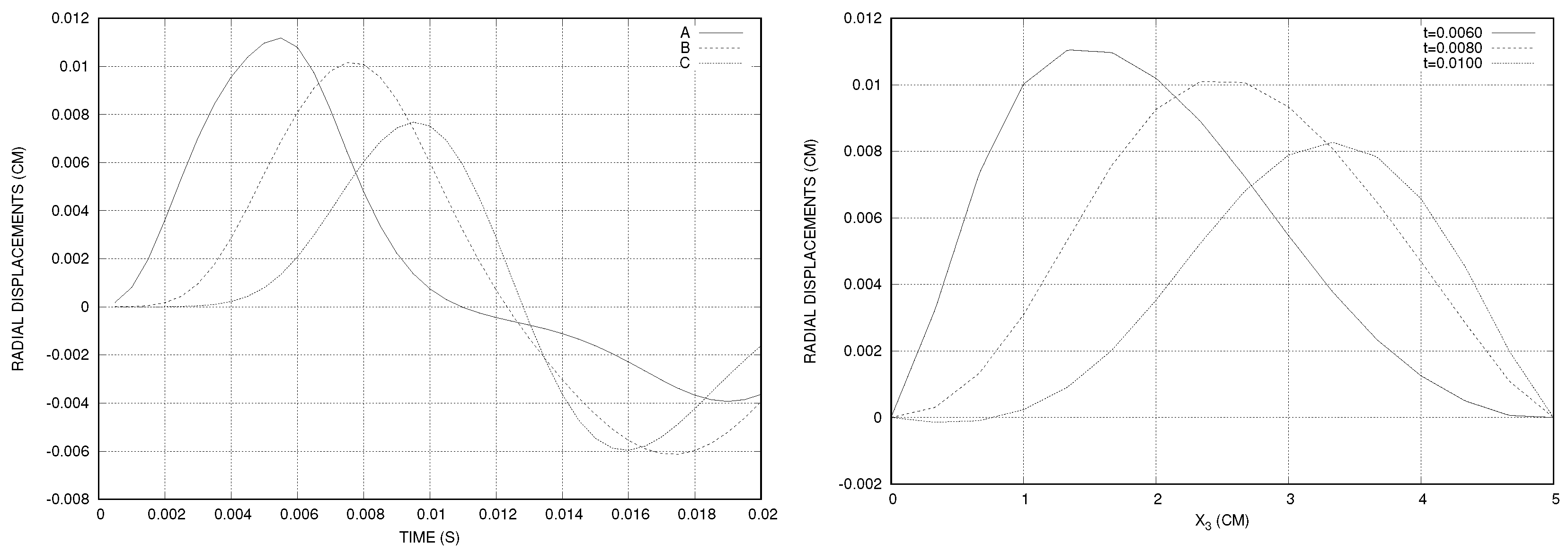
The time step was set to $\Delta t=0.0005$ s and the number of time steps to $N=40$. The radial displacement of the interface was measured at three points $A(R,0,L/4)$, $B(R,0,L/2)$, and $C(R,0,3L/4)$. We observed that the displacements were small, less than $0.012$ cm (see Figure 2, left). Similar results are observed in [41] using non-conforming meshes. In addition, we measured the radial displacement along the line $(R,0,x_3)$, $x_3\in [0,L]$ on the interface (see Figure 2, right.)

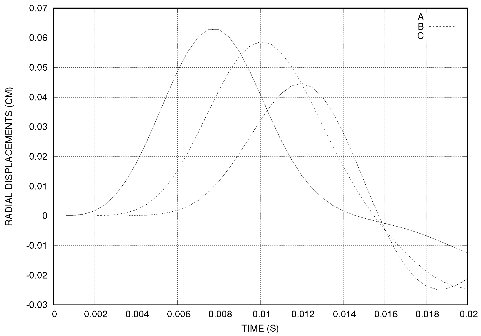
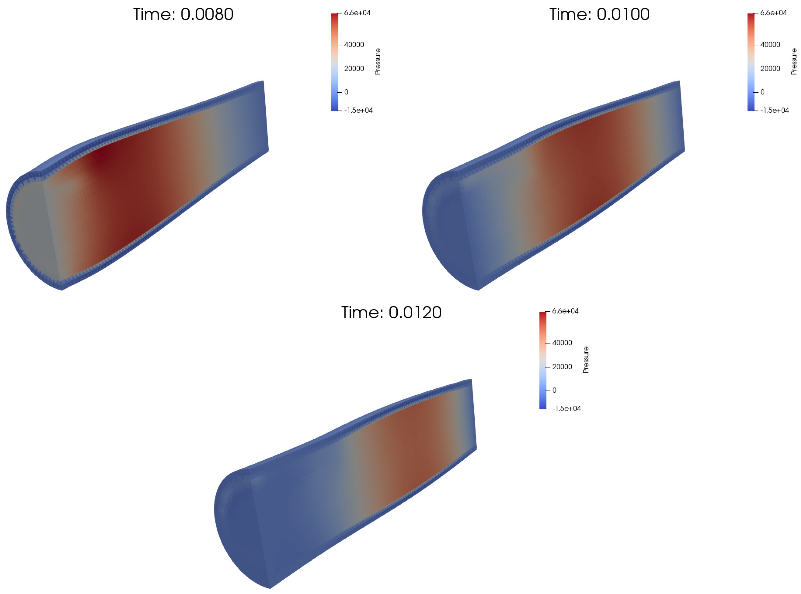
To obtain visible displacement, we also tested with the sin-like stress at the inlet:

$${\mathbf{h}}_{in}(\mathbf{x},t)=\left\{\begin{array}{ll}\left(0,0,5\times 1.3332\times {10}^4\times \frac{(1-cos(2\pi t/0.001\left)\right)}{2}\right),& \mathbf{x}\in {\Sigma }_1,0\le t\le 0.001\\ \left(0,0,0\right),& \mathbf{x}\in {\Sigma }_1,0.001\le t\le T\end{array}\right.$$

where $T=0.02$ s. The other parameters were the same. The displacements at three points are plotted in Figure 3 and the pressure at three time instants is plotted in Figure 4.

At each time step, we had to solve a sparse non-symmetric linear system for the fluid–structure velocity and pressure and a sparse symmetric positive definite linear system for the mesh displacement. The linear systems were solved using MUMPS (MUltifrontal Massively Parallel sparse direct Solver), implemented in FreeFem++. This method was very efficient; the total CPU time for the first three meshes were: 44 s (1.1 s/iteration) for Mesh 1, 173 s (4.3 s/iteration) for Mesh 2 and 1083 s (27 s/iteration) for Mesh 3, on a computer with a processor of 4 × 3.30 GHz frequency and 16 Go RAM. For Mesh 4, the CPU time was about 10 min/iteration on a noed Intel Sandy-Bridge 16 × 3.30 GHz and 64 Go RAM.

In [4], the mean number of iterations per time step is: 33.9 for the fixed-point with Aitken acceleration and 8.9 iterations for a quasi-Newton algorithm. At each iteration of quasi-Newton algorithm, a linear system is solved. In [41,42], the average number of Newton iterations per time step is 3.

6.2. Cane Cylinder

We considered the fluid–structure interaction in a cane-like geometry inspired from [4,43]. The parameters of the fluid domain were: $R=0.5$ cm, $R_1=1$ cm, $L_1=1$ cm, $L_2=5$ cm (see Figure 5, left). The fluid was surrounded by a structure of constant thickness $h^S=0.1$ cm.

The time step was $\Delta t=0.0005$ s, but the final time was $T=0.04$ s. The other parameters were the same as in the case of the straight cylinder. The details of meshes used for the numerical tests are presented in

Table 2. The number of vertices, tetrahedra and degrees of freedom (DOF) of fluid–structure linear system for each mesh.

	Vertices	Tetrahedra	DOF
Mesh 1	2079	9828	37,800
Mesh 2	3632	17,784	67,880
Mesh 3	5802	29,106	110,526

.

We measured the displacement of the interface ar three points: $U_1^S$ at $A(R_1+2R,0,0)$, $U_3^S$ at $B(0,0,R_1+2R)$ and $U_1^S$ at $C(-R_1-2R,0,0)$ (see Figure 6). The pressure at three time instants is plotted in Figure 7. We observed that, for the sin-like stress at the inlet, the structure displacements were greater than 0.23 (cm) and a non-linear model for the structure could be more appropriate. We chose a sin-like stress at the inlet with maximal value five times greater than the constant case to obtain visible deformations. Even though we used the same sin-like stress at the inlet, the structure displacements were larger than in the straight cylinder case because of the shape as well as because the cane was longer. Recall that the structure was fixed at both ends.

The total CPU time for the three meshes were: 255 s (3.18 s/iteration) for Mesh 1, 502 s (6.2 s/iteration) for Mesh 2 and 915 s (11.2 s/iteration) for Mesh 3, on a computer with a processor of 4 × 3.30 GHz frequency and 16 Go RAM.

In [4], the mean number of iterations per time step is 8.9 for quasi-Newton algorithm. The fixed-point algorithm with Aitken acceleration failed.

6.3. Artery Stenosis

Now, we considered a fluid–structure interaction in artery stenosis inspired from the paper [42]. The inlet and outlet surfaces ${\Sigma }_1$, ${\Sigma }_3$ were disks of radius R, normal to the axis $O{x}_1$ of centers $(x_{min},0,0)$ and $(x_{max},0,0)$, respectively. The lateral surface ${\Gamma }_0$ of the initial fluid domain was composed by the bottom half straight cylinder surface

$$\left\{(x_1,x_2,x_3)\in {\mathbb{R}}^3;x_{min}<x_1<x_{max},\sqrt{x_2^2+x_3^2}=R,x_3<0\right\}$$

and the stenosis surface (see Figure 8), obtained from the top half straight cylinder surface

$$\left\{(x_1,x_2,x_3)\in {\mathbb{R}}^3;x_{min}<x_1<x_{max},\sqrt{x_2^2+x_3^2}=R,x_3\ge 0\right\}$$

via the map

$$(x_1,x_2,x_3)\to \left(x_1,x_2,x_3-(h_{max}^S-h_{min}^S)\frac{({\ell }^2-x_1^2)}{{\ell }^2}\frac{(R^2-x_2^2)}{R^2}\right),|x_1|\le \ell ,|x_2|\le R.$$

The initial boundary of the structure domain was composed by: the interior lateral surface ${\Gamma }_0$, which is the fluid–structure interface; the exterior lateral surface

$${\Gamma }_0^N=\left\{(x_1,x_2,x_3)\in {\mathbb{R}}^3;x_{min}<x_1<x_{max},\sqrt{x_2^2+x_3^2}=R+h_{min}^S\right\};$$

and two annular surfaces ${\Sigma }_5$, ${\Sigma }_7$, of radii R and $R+h_{min}^S$, normal to the axis $O{x}_1$, of centers $(x_{min},0,0)$ and $(x_{max},0,0)$, respectively.

The numerical values were: $R=0.5$ cm, $x_{min}=-3,x_{max}=3$, $\ell =1.5$ cm, $h_{min}^S=0.1$ cm, and $h_{max}^S=0.5$ cm. The details of meshes used for the numerical tests are presented in

Table 3. The number of vertices, tetrahedra and degrees of freedom (DOF) of fluid–structure linear system for each mesh.

	Vertices	Tetrahedra	DOF
Mesh 1	5756	28,395	108,209
Mesh 2	20,970	95,202	369,486
Mesh 3	48,245	220,266	805,533
Mesh 4	92,228	425,872	1,554,300

.

We used the same sin-like stress at the inlet similar to the precedent experiments

$${\mathbf{h}}_{in}(\mathbf{x},t)=\left\{\begin{array}{ll}\left(0,0,mag\times 1.3332\times {10}^4\times \frac{(1-cos(2\pi t/0.001\left)\right)}{2}\right),& \mathbf{x}\in {\Sigma }_1,0\le t\le 0.001\\ \left(0,0,0\right),& \mathbf{x}\in {\Sigma }_1,0.001\le t\le T\end{array}\right.$$

where $T=0.02$ s and $mag>0$ is a parameter.

For Mesh 1, the time step was set to $\Delta t=5\times {10}^{-4}$ s, the number of time steps to $N=40$ and $mag=5$. The total CPU time was 323 s (8.07 s/iteration), on a computer with a processor of 4 × 3.30 GHz frequency and 16 Go RAM. The radial displacement of the interface was measured at three points: $A(-\ell ,0,R)$, $B(0,0,R-(h_{max}^S-h_{min}^S))$, and $C(\ell ,0,R)$ (see Figure 9). We observed that the maximal displacement of point A was more than 0.08 cm, which was more important than in the case of straight cylinder (see Figure 3). The artery deformation was more important in the uphill zone of the stenosis than in the case of healthy artery.

For Mesh 2, the time step was set to $\Delta t={10}^{-4}$ s, the number of time steps to $N=200$ and $mag=2$. The total CPU time was 15,123 s (75.6 s/iteration), on a noed Intel Sandy-Bridge 16 × 3.30 GHz and 64 Go RAM.

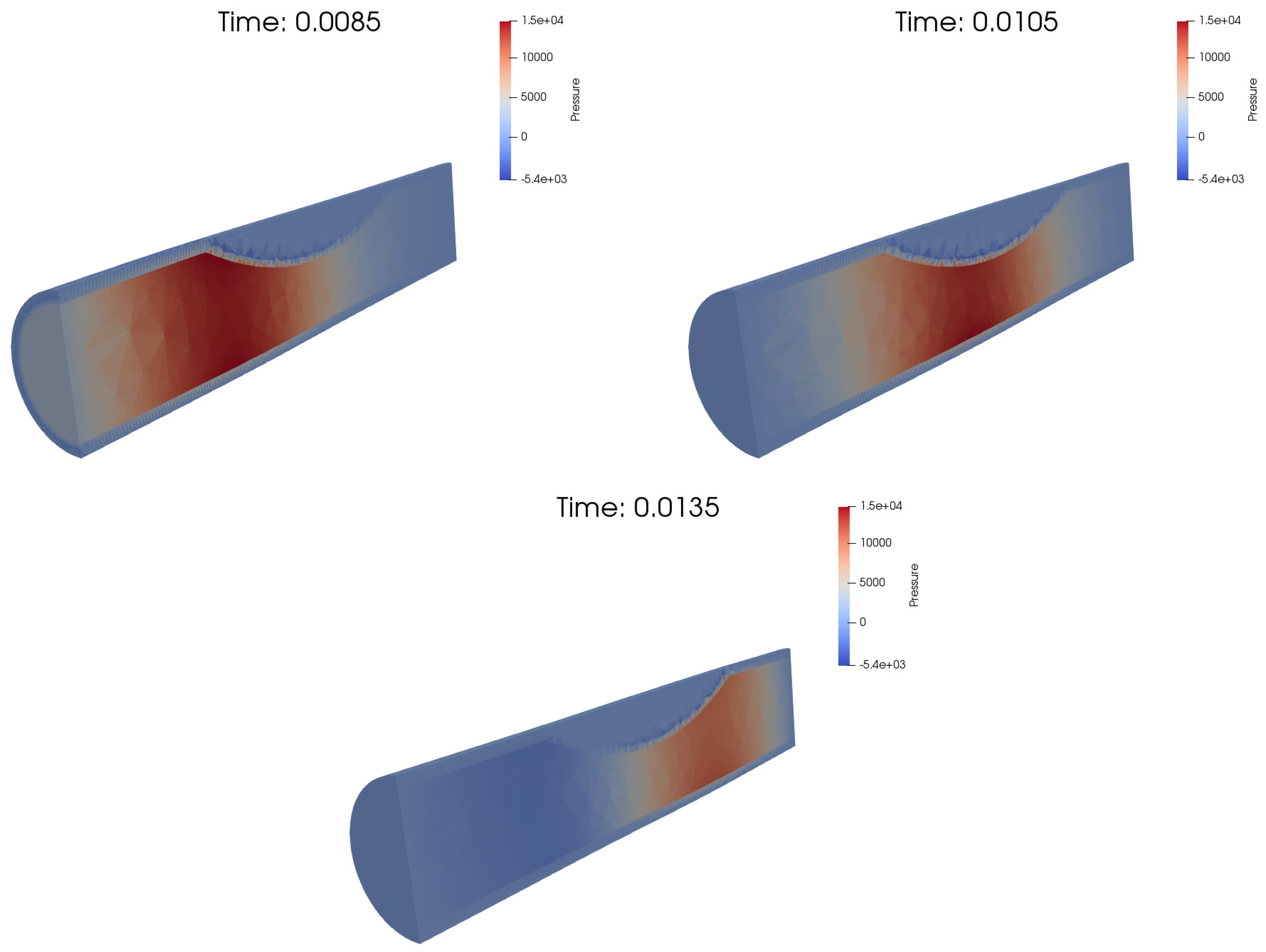
For Mesh 3, the time step was set to $\Delta t={10}^{-4}$ s, the number of time steps to $N=200$ and $mag=1$. The average CPU time was 4 min 55 s by iteration, on a noed Intel Sandy-Bridge 16 × 3.30 GHz and 64 Go RAM. The pressure at three time instants is plotted in Figure 10.

For Mesh 4, the time step was set to $\Delta t=5\times {10}^{-5}$ s, the number of time steps to $N=400$ and $mag=1$. The average CPU time was 18 min 8 s by iteration, on a noed Intel Sandy-Bridge 16 × 3.30 GHz and 64 Go RAM.

For finer mesh, we were forced to use smaller time steps. This phenomenon was observed for neither the three-dimensional tests presented above nor for the two-dimensional benchmark flow around a flexible thin structure attached to a fixed cylinder (see [37]). The semi-implicit algorithms had good stability properties (see Remark 3). We suppose that the source of the problem is this particular surface mesh of the stenosis zone obtained from the mesh of the top half straight cylinder surface by vertical projection on the stenosis surface.

7. Conclusions

We have presented a monolithic semi-implicit method for three-dimensional fluid–structure interaction problems. At each time step, we solve only a linear system to find the fluid–structure velocity and the fluid pressure, thus the method is fast. We use a global mesh for the fluid–structure domain where the fluid–structure interface is an interior boundary. Using globally continuous finite element for the velocity in the fluid–structure mesh, the continuity of velocity at the interface is automatically satisfied.

References

1. Le Tallec, P.; Mouro, J. Fluid structure interaction with large structural displacements. Comput. Methods Appl. Mech. Eng. 2001, 190, 3039–3067. [Google Scholar] [CrossRef]
2. Nobile, F. Numerical Approximation of Fluid-Structure Interaction Problems with Application to Haemodynamics. Ph.D. Thesis, EPFL, Lausanne, Switzerland, 2001. [Google Scholar]
3. Formaggia, L.; Gerbeau, J.-F.; Nobile, F.; Quarteroni, A. On the coupling of 3D and 1D Navier-Stokes equations for flow problems in compliant vessels. Comput. Methods Appl. Mech. Eng. 2001, 191, 561–582. [Google Scholar] [CrossRef]
4. Gerbeau, J.-F.; Vidrascu, M. A quasi-Newton algorithm based on a reduced model for fluid-structure interaction problems in blood flows. M2AN Math. Model. Numer. Anal. 2003, 37, 631–647. [Google Scholar] [CrossRef]
5. Fernàndez, M.A.; Moubachir, M. A Newton method using exact jacobians for solving fluid-structure coupling. Comput. Struct. 2005, 83, 127–142. [Google Scholar] [CrossRef]
6. Dettmer, W.; Perić, D. A computational framework for fluid-structure interaction: Finite element formulation and applications. Comput. Methods Appl. Mech. Eng. 2006, 195, 5754–5779. [Google Scholar] [CrossRef]
7. Murea, C.M. Numerical simulation of a pulsatile flow through a flexible channel. ESAIM Math. Model. Numer. Anal. 2006, 40, 1101–1125. [Google Scholar] [CrossRef]
8. Mbaye, I.; Murea, C.M. Numerical procedure with analytic derivative for unsteady fluid-structure interaction. Commun. Numer. Meth. Eng. 2008, 24, 1257–1275. [Google Scholar] [CrossRef]
9. Kuberry, P.; Lee, H. A decoupling algorithm for fluid-structure interaction problems based on optimization. Comput. Methods Appl. Mech. Eng. 2013, 267, 594–605. [Google Scholar] [CrossRef]
10. Hubner, B.; Walhorn, E.; Dinkler, D. A monolithic approach to fluid-structure interaction using space-time finite elements. Comput. Meth. Appl. Mech. Eng. 2004, 193, 2087–2104. [Google Scholar] [CrossRef]
11. Hron, J.; Turek, S. A monolithic FEM/multigrid solver for an ALE formulation of fluid-structure interaction with application in biomechanics. In Fluid-Structure Interaction; Lecture Notes in Computational Science and Engineering 53; Springer: Berlin, Germany, 2006; pp. 146–170. [Google Scholar]
12. Dunne, T. An Eulerian approach to fluid-structure interaction and goal-oriented mesh adaptation. Int. J. Numer. Methods Fluids 2006, 51, 1017–1039. [Google Scholar] [CrossRef]
13. Heil, M.; Hazed, A.L.; Boyle, J. Solvers for large-displacement fluid-structure interaction problems: Segregated versus monolithic approaches. Cumput. Mech. 2008, 193, 91–101. [Google Scholar] [CrossRef]
14. Pironneau, O. Numerical study of a monolithic fluid-structure formulation. In Variational Analysis and Aerospace Engineering; Springer Optimization and Its Applications 116; Springer: Cham, Seitzerland, 2016; pp. 401–420. [Google Scholar]
15. Hecht, F.; Pironneau, O. An energy stable monolithic Eulerian fluid-structure finite element method. Int. J. Numer. Methods Fluids 2017, 85, 430–446. [Google Scholar] [CrossRef]
16. Chiang, C.-Y.; Pironneau, O.; Sheu, T.W.H.; Thiriet, M. Numerical Study of a 3D Eulerian Monolithic Formulation for Incompressible Fluid-Structures Systems. Fluids 2017, 2, 34. [Google Scholar] [CrossRef]
17. Pironneau, O. An energy stable monolithic Eulerian fluid-structure numerical scheme. Chin. Ann. Math. Ser. B 2018, 39, 213–232. [Google Scholar] [CrossRef]
18. Donea, J. Arbitrary Lagrangian-Eulerian finite element methods. In Computational Methods for Transient Analysis; Belytschko, T., Hughes, T.J.R., Eds.; North-Holland: Amsterdam, The Netherlands, 1983; pp. 474–516. [Google Scholar]
19. Quarteroni, A.; Formaggia, L. Mathematical modelling and numerical simulation of the cardiovascular system. In Handbook of Numerical Analysis, Vol. XII; Ciarlet, P.G., Ed.; North-Holland: Amsterdam, The Netherlands, 2004; pp. 3–127. [Google Scholar]
20. Peskin, C.S. The immersed boundary method. Acta Numer. 2002, 11, 479–517. [Google Scholar] [CrossRef] [Green Version]
21. Glowinski, R.; Hesla, T.I.; Joseph, D.; Pan, T.; Périaux, J. A distributed Lagrange multiplier/fictitious domain method for the simulation of flow around moving rigid bodies: Application to particulate flow. Comput. Meth. Appl. Mech. Eng. 2000, 184, 241–267. [Google Scholar] [CrossRef]
22. Boffi, D.; Gastaldi, L. A fictitious domain approach with Lagrange multiplier for fluid-structure interactions. Numer. Math. 2017, 135, 711–732. [Google Scholar] [CrossRef]
23. Bost, C.; Cottet, G.-H.; Maitre, E. Convergence analysis of a penalization method for the three-dimensional motion of a rigid body in an incompressible viscous fluid. SIAM J. Numer. Anal. 2010, 48, 1313–1337. [Google Scholar] [CrossRef]
24. Yakhlef, O.; Murea, C.M. Numerical procedure for fluid-structure interaction with the structure displacements limited by a rigid obstacle. Appl. Comput. Mech. 2017, 11, 91–104. [Google Scholar] [CrossRef]
25. Court, S.; Fournié, M.; Lozinski, A. A fictitious domain approach for fluid-structure interactions based on the extended finite element method. In Proceedings of the SMAI Congress 2013 6th French Biennale of Applied and Industrial Mathematics, Seignosse, France, 27–31 May 2013; pp. 308–317. [Google Scholar]
26. Court, S.; Fournié, M. A fictitious domain finite element method for simulations of fluid-structure interactions: The Navier-Stokes equations coupled with a moving solid. J. Fluids Struct. 2015, 55, 398–408. [Google Scholar] [CrossRef]
27. Alauzet, F.; Fabrèges, B.; Fernández, M.A.; Landajuela, M. Nitsche-XFEM for the coupling of an incompressible fluid with immersed thin-walled structures. Comput. Methods Appl. Mech. Eng. 2016, 301, 300–335. [Google Scholar] [CrossRef] [Green Version]
28. Boffi, D.; Hecht, F.; Pironneau, O. Distributed Lagrange multiplier for fluid-structure interactions. In Numerical Methods for PDEs; Di Pietro, D., Ern, A., Formaggia, L., Eds.; SEMA SIMAI Springer Series; Springer: Berlin/Heidelberg, Germany, 2018; pp. 129–145. [Google Scholar]
29. Wang, Y.; Jimack, P.; Walkley, M. A one-field monolithic fictitious domain method for fluid-structure, interactions. Comput. Methods Appl. Mech. Eng. 2017, 317, 1146–1168. [Google Scholar] [CrossRef]
30. Wang, Y.; Jimack, P.; Walkley, M. Energy analysis for the one-field fictitious domain method for fluid-structure interactions. Appl. Numer. Math. 2019, 140, 165–182. [Google Scholar] [CrossRef] [Green Version]
31. Fernàndez, M.A.; Mullaert, J.; Vidrascu, M. Explicit Robin-Neumann schemes for the coupling of incompressible fluids with thin-walled structures. Comput. Methods Appl. Mech. Eng. 2013, 267, 566–593. [Google Scholar] [CrossRef]
32. Dettmer, W.; Perić, D. A new staggered scheme for fluid-structure interaction. Int. J. Numer. Meth. Eng. 2013, 93, 1–22. [Google Scholar] [CrossRef]
33. Fernàndez, M.A.; Gerbeau, J.-F.; Grandmont, C. A projection semi-implicit scheme for the coupling of an elastic structure with an incompressible fluid. Int. J. Numer. Methods Eng. 2007, 69, 794–821. [Google Scholar] [CrossRef]
34. Murea, C.M.; Sy, S. A fast method for solving fluid-structure interaction problem numerically. Int. J. Numer. Meth. Fluids 2009, 60, 1149–1172. [Google Scholar] [CrossRef]
35. Sy, S.; Murea, C.M. A stable time advancing scheme for solving fluid-structure interaction problem at small structural displacements. Comput. Meth. Appl. Mech. Eng. 2008, 198, 210–222. [Google Scholar] [CrossRef]
36. Murea, C.M.; Sy, S. Updated Lagrangian/Arbitrary Lagrangian Eulerian framework for interaction between a compressible Neo-Hookean structure and an incompressible fluid. Int. J. Numer. Meth. Eng. 2017, 103, 1067–1084. [Google Scholar] [CrossRef]
37. Murea, C.M. Monolithic algorithm for dynamic fluid-structure interaction problem. In Mathematical Modelling in Solid Mechanics; Dell Isola, F., Sofonea, M., Steigmann, D., Eds.; Advanced Structured Materials 69; Springer: Singapore, 2017; pp. 135–146. [Google Scholar]
38. Sy, S.; Murea, C.M. Algorithm for solving fluid-structure interaction problem on a global moving mesh. Coupled Syst. Mech. 2012, 1, 99–113. [Google Scholar] [CrossRef]
39. Ciarlet, P.G. Élasticité Tridimensionnelle; Masson: Paris, France, 1986. [Google Scholar]
40. Hecht, F. New development in FreeFem++. J. Numer. Math. 2012, 20, 251–265. [Google Scholar] [CrossRef]
41. Deparis, S.; Forti, D.; Quarteroni, A. A Fluid-Structure Interaction Algorithm Using Radial Basis Function Interpolation Between Non-Conforming Interfaces. In Advances in Computational Fluid-Structure Interaction and Flow Simulation; Bazilevs, Y., Takizawa, K., Eds.; Springer: Berlin/Heidelberg, Germany, 2016; pp. 439–450. [Google Scholar]
42. Forti, D.; Bukac, M.; Quaini, A.; Canic, S.; Deparis, S. A monolithic approach to fluid-composite structure interaction. J. Sci. Comput. 2017, 72, 396–421. [Google Scholar] [CrossRef]
43. Lefieux, A.; Auricchio, F.; Conti, M.; Morganti, S.; Reali, A.; Trimarchi, S.; Veneziani, A. Computational Study of Aortic Hemodynamics: From Simplified to Patient-Specific Geometries. In Advances in Computational Fluid-Structure Interaction and Flow Simulation; Bazilevs, Y., Takizawa, K., Eds.; Modeling and Simulation in Science, Engineering and Technology; Springer: Berlin/Heidelberg, Germany, 2016; pp. 397–407. [Google Scholar]
Figure 1. Initial geometrical configuration.
Fluids 04 00094 g001
Figure 2. Constant stress at the inlet: the time history of the displacement of three points on the interface (left); and the radial displacement at time instants t = 0.0060 , t = 0.0080 , t = 0.0100 (right).
Fluids 04 00094 g002
Figure 3. The time history of the displacement of three points on the interface using sin-like stress at the inlet.
Fluids 04 00094 g003
Figure 4. The pressure obtained with Mesh 4 using sin-like stress at the inlet.
Fluids 04 00094 g004
Figure 5. The parameters of the fluid domain (left); and a global mesh for fluid–structure domain (right).
Fluids 04 00094 g005
Figure 6. The time history of the displacement of three points on the interface using constant (left) and sin-like (right) stress at the inlet.
Fluids 04 00094 g006
Figure 7. The computed pressure obtained with sin-like stress at the inlet (Mesh 2).
Fluids 04 00094 g007
Figure 8. The stenosis interface.
Fluids 04 00094 g008
Figure 9. The time history of the displacement of three points on the interface using sin-like stress at the inlet (Mesh 1).
Fluids 04 00094 g009
Figure 10. The computed pressure obtained with Mesh 3.
Fluids 04 00094 g010