Article

Heat Convective Effects on Turbulence and Airflow inside an B767 Aircraft Cabin

School of Engineering Technology, Purdue University, West Lafayette, IN 47907, USA
Fluids 2019, 4(3), 167; https://doi.org/10.3390/fluids4030167
Submission received: 15 June 2019 / Revised: 11 August 2019 / Accepted: 5 September 2019 / Published: 8 September 2019
(This article belongs to the Special Issue Turbulence and Transitional Modeling of Aerodynamic Flows)

Abstract

:
Thermal plumes generated by human bodies can affect the temperature and humidity of the surrounding environment. An experimental study investigated the effects of thermal plumes formed by aircraft passengers on airflow and turbulence characteristics inside aircraft-cabins. An 11-row, wide-body B767 cabin mockup was used with actual seats, air diffusers and cabin profile. Thermal manikins were used simulating passengers in the cabin. Tracer gas and air speed inside the cabin were measured while the heat from the manikins was turned on and off to help understand the effects of the thermal heat released by the manikins. Results showed that tracer gas distribution were more uniformly and equally distributed around the release source and the air speed fluctuation were lower under cooler environments when the thermal manikins were turned off. Heated environments increased the values of turbulence kinetic energy and the turbulence intensity levels. However, the effects on the turbulence intensity were less significant compared to the turbulence kinetic energy. On the other hand, the dissipation rates were higher for unheated cases in the front and back sections of the mockup cabin. The relative uncertainty for tracer gas sampling ranged between ±5–14% for heated manikins versus ±8–17% for unheated manikins. Higher uncertainty levels accompanied the turbulence measurements due to the highly chaotic nature of the flow inside the cabin.

1. Introduction

Several studies have been conducted to understand air quality, airflow characteristics and human thermal comfort inside aircraft cabins. Investigations used various experimental and analytical techniques such as particle image velocimetry (PIV), particles dispersion, computational fluid dynamics (CFD), and tracer gas.
The effect of air nozzle sizes and direction on the airflow inside aircraft cabin was investigated in 2006 by Lebbin et al. [1] inside a generic room using stereoscopic PIV techniques. The generic room was described by Lin et al. [2]. Reynolds number was held constant at the inlet slot of the room with a value of approximately 2226. It was noted that the center of rotation of the overall airflow significantly changed with a change in the size of the air inlet slot size, whereas the turbulence levels in the room was not affected significantly since Reynolds number was not changed [1].
Large Eddy Simulation (LES) and Reynolds Averaged Navier–Stokes (RANS) methods were used by Ebrahimi et al. [3] to understand the airflow and turbulence characteristics inside an 11-row B767 cabin mockup. The simulation results were validated against available experimental data. The studies showed that LES with Werner–Wengle wall function could predict unsteady airflow velocity fields inside the cabin mockup with high accuracy. On the other hand, when air circulation was present, the RGN k-ꜫ model with a non-equilibrium wall function model predicted the airflow velocities with good agreements against experimental results. In a later study by Ebrahimi et al. [4], tracer gas and particle dispersion inside the same 11-row B767 cabin mockup was predicted. The initial airflow velocities exiting the supply nozzles were experimentally measured using omni-probes. Three different grid sizes were examined for grid uncertainty.
The effect of gaspers on the airflow inside a Boeing 767 cabin was investigated using tracer gas. The tracer gas was released and sampled around the nasal area of a seated passenger a thermal manikin represented with a thermal manikin. The personal supply gaspers were found to have some effect on the contaminant plume inside the cabin impacting the local exposure around the release zone. It was also found that there was significant reduction in close-range, person-to-person exposure, while in other cases there was negligible or even negative impacts [5].
Local ventilation effectiveness inside an 11-row B767 cabin mockup and in a 5-row section of a salvaged B737 passenger cabin was investigated by [6] and [7], respectively. Tracer gas was used as the tracing agent during the experiments in both cabins. For the 11-row B767 cabin mockup, the tracer gas, which was mainly composed of CO2, was sampled in all seats. The overall ventilation rate was found approximately at 27 air changes per hour (ACH) based on total supply air flow. The ventilation effectiveness ranged from 0.86 to 1.02 with a mean value of 0.94. These ventilation effectiveness values were higher than what typically is found in other indoor environments. This gain in effectiveness is likely due to the relatively high airspeeds that can improve mixing rates. On the other hand, experiments inside the 5-row sectional B737 were carried with similar thermal manikins as was used in the B767 cabin mockup. Local ventilation effectiveness was found to be uniform throughout the B737 cabin regardless of the location inside the cabin. For gaseous transport, similar conclusions were found in both cabins, B767 and B737, where gaseous transport was significantly transported in the transverse and longitudinal directional of the cabins.
Outbreaks of Severe Acute Respiratory Syndrome (SARS) and H1N1-swine flu can cause serious hazardous and threats to humans due to the large number of passengers using airplanes. In 2002, it was believed that a person infected with SARS led to 22 other passengers being infected during a flight from Hong Kong to Beijing. Furthermore, concerns of possible terrorist attacks onboard commercial flights have significantly risen due to the use of the nerve agent to attack the Tokyo subway in 1995 and the anthrax cases in Florida and Washington, D.C. in 2001. Consequently, it became considerably important to understand particulates dispersion behavior inside aircraft cabins, develop means for detecting undesirable components inside aircraft cabins and to find methods for preventing the aircraft from being used for intentional contaminant deployment [8]. The potential of contaminating aircraft cabins with oil and hydraulic fluids was recognized by the Committee on Aviation Toxicology (CAT) of the Aero Medical Association acknowledged shortly after the introduction of bleed air system [9]. The concentration of airborne contaminants inside aircraft cabins is expected to vary depending on aircraft type, specific airline maintenance practices, and bleed air source already too old [10]. Frequency of bleed air contamination incidents were estimated between 0.09 to 3.88 incidents per a thousand flight cycles, according to [11], which could mean 2–3 bleed air incidents per day. Another study by [8] indicated that there might be 0.2–0.8 incidents per thousand flights according to incidents reported by the US Federal Aviation Administration (FAA), Department of Transportation, NASA and flight attendant association databases [12]. Thus, it is important to understand the airflow characteristics inside aircraft cabins to help in preventing and minimizing bacterial and viral spreads or intentional nerve attacks onboard air flights. Previous studies have investigated bacterial, particulate and gaseous dispersion inside passenger aircraft flights under normal operating conditions mostly assuming fully occupied cabins. However, since airplanes are not always fully occupied and since heat released by the passengers can affect the indoor airflow and air quality as they generate thermal plumes, it was important to investigate the effect of such variables on the airflow characteristics inside the cabin. Thermal plumes can significantly influence indoor airflow distribution as well as indoor air quality. Aircraft passenger cabins are occupied by humans whose body released heat can rise both temperature and humidity. This rise can affect the velocity and the airflow distribution inside aircraft cabins. A change in the number of passengers, such as in a partially full flight, can affect the convective transport mechanism inside the aircraft cabin. For these reasons, this study analyzed the effects of heat generated by passengers on the airflow and turbulence characteristics inside a B767 aircraft cabin mockup using thermally heated manikins. The study used tracer gas, mainly composed from carbon dioxide, to track the airflow inside the cabin. Air speed transducers were used to measure the speed at various locations inside the cabin. Tracer gas and air speed were collected when the cabin mockup was assumed to be fully equipped or empty by running electric current in thermal wires wrapped around the thermal manikins on and off for each case.
The study will provide experimental data for researchers to better understand the airflow characteristic inside aircraft cabins as well as airline manufacturers who might have to modify their designs. The study also provides some data necessary for computational fluid dynamics work to help in developing “user-defined functions” (UDF) and to validate some simulations on the same aircraft model and type.

2. Background

To analyze turbulence characteristics of a fluid, the k–ε model is one of the most frequently used models utilizing two diffusive equations. The first one modeling the turbulent kinetic energy “k” and the second one modeling the dissipate rate “ε” as shown in Equations (1) and (2), respectively:
t ( ρ k ) + x i ( ρ k u i Γ ( k ) k x i   ) = ρ ( P ( k ) ε ) ,
t ( ρ ε ) + x i (   ρ ε u i Γ ( ε ) ε x i   ) = ρ ( C ε 1 P ( k ) ε C ε 2 ) ε k ,

Rate of Change Advection Diffusion Source

where Γ ( k ) =   μ +   μ T   σ k ; Γ ( ε ) =   μ +   μ T   σ ε . μ T is the turbulence dynamic viscosity, P ( k ) is the turbulence production rate, ui is the velocity vector, and ρ is the density. Values for the different empirical constants were proposed by Launder and Spalding in 1974 [13] and were given as C ε 1 = 1.44 ; C ε 2 = 1.92 ; σ ϵ = 1.3 ; σ k = 1 ;   P ( k ) =   u v ¯ u y =   μ T   ρ ( u y ) 2 or u i u j ¯ u i x j , where u   a n d   v are the fluctuating components of the velocities in two-dimensional flow. These values were based on extensive examination of free turbulent flows, but they cannot be used for wall flows. Thus, this model is applicable only to flows or flow regions with high turbulence rates and cannot be applied near walls, where viscous effects become dominant. For such situations, a near wall function approach is usually used.
Assuming that the turbulence was isotropic, the turbulence kinetic energy “k” in its tensor format in Equation (3) reduces to Equation (4), where v’ is the isotropic speed fluctuation part:
k = 1 2 u i u i ¯ ,
which reduces to
k =   3 2 ( v ) 2
Kolmogorov formulated the hypothesis of local isotropy based on definitions of local homogeneity and isotropy. This hypothesis postulates that at large Reynolds numbers all the symmetries of the Navier–Stokes equations are restored in the statistical sense [14]. The local dissipation rate as a function of the local strain created by the flow is then given in Equation (5) [14]:
ε =   γ S i j S i j ,
where Sij is the strain defined in Equation (6). Thus, the local dissipation rate “ ε ” becomes according to Taylor dissipation rate for isotropic flow as given in Equation (7), where v is the isotropic local speed and A is an empirical constant (approximately = 15) [14]:
S i j = 1 2 ( U i x j + U j x i ) ,
ε = A γ ( v x ) 2 ¯ .

3. Experimental Setup

3.1. Testing Facility

A full-scale aircraft mockup with dimensions of 9.6 m in length and 4.7 m in width was used to conduct the testing. The aircraft cabin mockup was one of the largest available research mockup cabins in its class and it modelled a B767, 11-row aircraft cabin. Each row consisted of seven seats in the transverse direction. The seats, air supply ducts, and diffusers were all utilized from salvaged B767 aircrafts. To simulate heat gains by a seated passenger, 10 m wire heater elements were wrapped and distributed around manikins that were seated in each seat inside the cabin mockup. The heat gain by each manikin was approximately 100 Watts similar to that released by a seated human [15]. The heat for each manikin could be turned on or off by cutting the electrical supply to each manikin. Fresh air was conditioned (cooled or heated) and filtered inside a set of HEPA (high efficiency particulate air) filters before was supplied to the cabin. The diffusers supplying air to the cabin were linear and had a decreasing supply duct upstream that balanced the air pressure across the diffusers. The exterior and interior of the cabin mockup along with the cooling and heating loops are shown in Figure 1.
The air supplied into the cabin was according to [16] standards supplying 8.57 L/s (18 ft3/min or CFM) per passenger seat. This made the total supplied air to the cabin 660 L/s (1400 CFM). The mockup cabin was supplied with 100% outside air, conditioned to 15.6 °C (60 F) at the upstream of the cabin main supply duct shown in Figure 1a (Air Inlet Supply Duct point). The outdoor air temperature was conditioned to the desired set point using an electric hear and water-glycol loops. The temperature at the main cabin supply duct was measured using an Omega 3-wire RTD model PR-10-2-100-1/4-6-E sensor (Norwalk, CT, USA). The humidity of the air was treated in a Munter dehumidifier (Amesbury, MA, USA).
The air temperature was conditioned to 15.6 °C (60 °F) at the duct entering the cabin, as shown in Figure 1a. The temperature inside the cabin was monitored, with the manikin heat on, using twenty-four thermocouples along the cabin interior surfaces, distributed evenly between the left and right side, and along the vertical height using 12 more thermocouples. The average temperature of all thermocouples ranged between 19–24 °C. The temperature ranges came into agreement with O’Donnell et al. [17] who reported that temperature onboard passenger aircraft cabins ranges between 19–23 °C. Before conducting any testing, it was necessary to ensure the uniformity of the air exiting the two linear diffusers shown in Figure 1c. The air exited the cabin through two exit openings along the bottom side of the walls on each side of the cabin mockup.

3.2. Tracer Gas Testing Setup and Methodology

Tracer gas mixture made up of 62.4% CO2 and 37.6% helium was used as the tracer gas agent in the experiments. The tracer gas was released in different seats inside the cabin though a 25.4 mm diameter copper tube. The mass flow of each of the two gases was controlled using two mass flow controllers (model MKS 1559A-200L-SV-S for CO2 and MKS 2179A-00114-CS-18V for He). The flow controllers were controlled by an Agilent DAQ system (model 34970A) (Santa Clara, CA, USA), MKS PR4000 power supply and RS-232 interface unit. The tracer gas was sampled using PP-Systems CO2-analyzers (Amesbury, MA, USA). The analyzers contained non-dispersive infrared sensors. To increase the simultaneous collection frequency during each test, a collection tree was connected to the inlet of the tracer gas analyzer. The tree had four ports and were distanced from each other so each port would be in the same seat in consecutive rows. This enabled all four ports of the sampling tree to be utilized in four separate seat locations (in consecutive rows) during a single experiment. LabVIEW (LabView6.1) was used to operate the Agilent DAQ, the interface unit and the mass flow controllers. It was designed to allow sequential collection from the first port until the fourth one. The tracer gas release tube and the collection tree are shown in Figure 2. The tip of the collection ports was fixed at a height of 1.23 m from the cabin floor. Tracer gas was released at very low speeds (approximately 0.53 ± 0.02 m/s) to minimize the disturbance to the airflow inside the cabin caused by the gas injection. To normalize the tracer gas sampled inside the cabin, two more CO2-analyzers were used. One was installed to sample the inlet CO2 at with the air coming through supply duct and another one analyzing the tracer gas leaving the cabin through the exhaust fans that are shown in Figure 1a.
Previous smoke visualization testing inside the cabin was done by [10] to decide on the best locations where tracer gas needed to be released. The airflow inside the cabin was shown to be very chaotic and thus the testing and visualization scenarios were repeated multiple times to decide on best local flow patterns. The smoke tracks along with the used tracer gas release locations are shown in Figure 3. The tracer gas was generally collected in the same row of release, three rows to the back and three rows to the front of the release row. The decision to cover three rows in each direction away from the release row was based on results from [18] who concluded that particles and tracer gas dispersion are significantly reduced beyond 3-rows. The released particles or tracer gas would be present beyond the 3-row limit, but in very small concentrations. In this study, tracer gas was injected continuously during each test for a total duration of 20-min. Samples were collected in each port of the sampling tree every 5 s resulting in 240 samples for each port or seat. Each 20-min sampling test was repeated in each seat three times for statistical consistency. With the 8-release locations were distributed around the cabin and with sampling done three to four rows to the front and three to four rows to the back, in mostly every seat in the transverse direction of each row, the data collected provided strong indication for the tendency of the tracer gas movement inside the cabin.
To ensure steady state conditions inside the cabin prior to any testing, it was estimated that 5 min were enough to exhaust any available CO2 from the background of the cabin remaining previous tests, from any person entering into the cabin to modify the sampling tree or entering through the cabin doors. Thus, after 5 min, the tracer gas was released sequentially in each of the eight seats shown in Figure 3.
To investigate the effects of heat generated by each manikin inside the cabin, the same tests were run but with no heat released by the manikins by cutting the electrical source into them.

3.3. Turbulence Characteristics Investigation Setup

A spherical omni-directional TSI velocity transducer (8475 series model) was used inside the cabin to measure and record the speed of the air. This would help in evaluating the turbulence intensity (TI) and turbulence kinetic energy (k). The speed transducer had a 5 s response time and its averaged uncertainty was estimated to be ±1%. The spherical transducer was fixed at a height of 1.23 m above the cabin floor in each seat across the cabin similar to where the tracer gas was sampled in. The probe is shown in Figure 4. Similar to the tracer gas testing, a 5-min waiting period was used prior to any data collection. The measured speed was used to estimate the turbulence intensity and the turbulence kinetic energy. Speed tests were done with heated and unheated manikins to check on the effects of the thermal plumes caused by the heated manikins on the turbulence characteristics inside the cabin.
Assuming isotropic flow, the TI and k were calculated as shown in Equations (4) and (8), respectively, where v is the fluctuating part of the speed and V ¯ is the average speed:
T I =   v 2 ¯ V ¯ .
The heat dissipation rate was numerically evaluated by discretizing Equation (7) and by implementing three omni-transducers, as shown in Equation (9). The middle transducer was represented as “i” and those in front and back were represented as “i + 1” and “i − 1”, respectively:
ε = 15 γ ( v i + 1   v i 1 2 Δ x ) 2 .
The separation distance “ Δ x ” was the distance between two consecutive transducers and γ was the kinematic viscosity of the air inside the cabin. The optimal separation distance Δ x was investigated to maintain minimal numerical errors. Five separation distances were considered between 5–25 cm. It was found that a separation distance of 12.7 cm was the best option providing the least numerical errors.

4. Results and Discussion

Tracer gas testing and speed measurements were done and repeated while having the electrical source supplying the thermal wires around the manikins turned on and off. With heated manikins, the temperature inside the cabin ranged between 19–23 °C, whereas, with unheated manikins, this air temperature dropped to 14–15 °C. The sampled CO2 through the analyzers in the cabin was normalized against the inlet and exit CO2 concentrations. This normalization is shown in Equation (10), where C is the sampled concentration of CO2, and the subscript n stands for normalized value:
C n =   C c a b i n   C i n l e t   C e x i t   C i n l e t .
Results for the normalized tracer gas and turbulence characteristics inside the B767 cabin mockup were published with more analysis and details in [19]. This paper focuses on similar results but when no heat was dissipated from the manikins and compares the results to the heated cases. Any time the term “heated” was used, it meant that the manikins were heated or the thermal wires were switched-on and similarly when “unheated” term was used then that meant the thermal wires were switched off and cutting any heat dissipation by the manikins.
The heated cabin testing resulted in multiple circulations inside the cabin [19]. The 2D circulations at a height of 1.23 m from the cabin floor are shown in Figure 5.
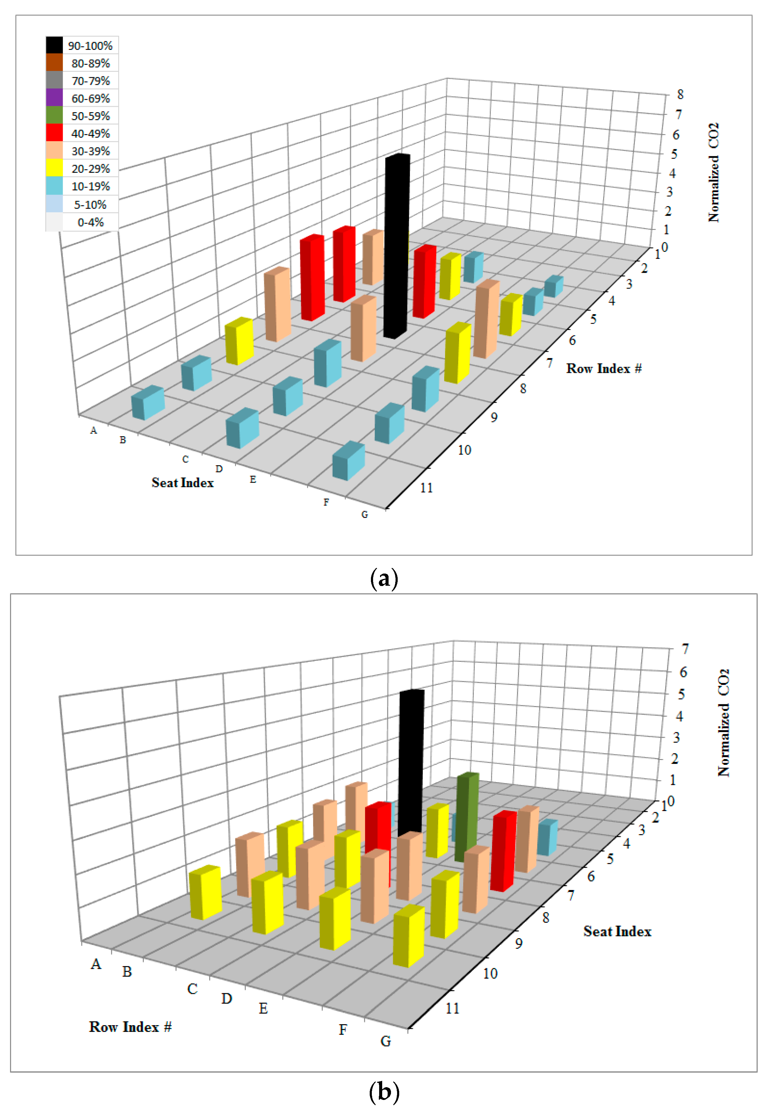
Normalized tracer gas distribution results for heated and unheated cases when releasing in seats 2D and 7D are presented in Figure 6a,b and Figure 7a,b), respectively. All individual test results for the heated manikins were published in [19]. For either case, heated or unheated, the results of more than one release location were combined together to conclude the behavior of the flow in specific sections inside the cabin mockup. For heated cases, based on results for release in seats 2D (Figure 6a) and 5B, a major drift in the front section of the cabin from east to west side was observed. On the other side, tracer gas analysis for release in seat 5D and seat 4F showed a major drift in the front-west side towards the east side. Moving further to the back section of the cabin and considering results for release in seat 7D (Figure 7a), another drift from the west to the east side of the cabin was concluded. The final combined analysis of the results was discussed in detail in [19] and showed the behavior shown in Figure 5. The smoke visualization results shown in Figure 3 (red lines), which were conducted with heated manikins, and the tracer gas results shown in Figure 5 both concluded the existence of multiple circulations inside the cabin mockup. Based on tracer gas results and analysis, the length of these circulations was shown to depend on the integral length scale of the cabin in each region. With a cabin length of 9.6 m, width 4.7 m and height of approximately 2 m, isotropic circulations with dimensions between 2 to 4 m were concluded. The dimensions of the circulations at a height of 1.23 m above the floor are shown in Figure 5.
The unheated tracer gas results, which were conducted with temperatures 6 °C less than the heated cases, showed more uniformly and symmetrically distributed tracer gas around the release location, especially when it was released in the centerline seats of the cabin as shown in Figure 6b and Figure 7b. In all of the release cases, the normalized tracer gas samples did not favor any side of the cabin over the other as was contrarily observed with heated cases such as in Figure 6a and Figure 7a.
All of the above analysis checked the dispersion at a height of 1.23 m; it was important to check any significant differences at different heights inside the cabin. Tracer gas vertical exposure was done in the east and west aisles in the front and middle sections of the cabin mockup. For the front part, the tracer gas was released in row 2 and collected in the same row but in the east and west aisles, whereas, for the middle part, the tracer gas was released in row 5 and collected in the east and west aisles of rows 4 and 6. The results for both heated and unheated results are shown in Table 1. More uniform results or smaller variability were seen with unheated than with heated environments, except in the lower regions near the floor. The non-uniform distribution in the lower sections of the cabin near the floor was expected due to many disturbances such as seats and manikins.

Turbulence Characteristics Results and Analysis

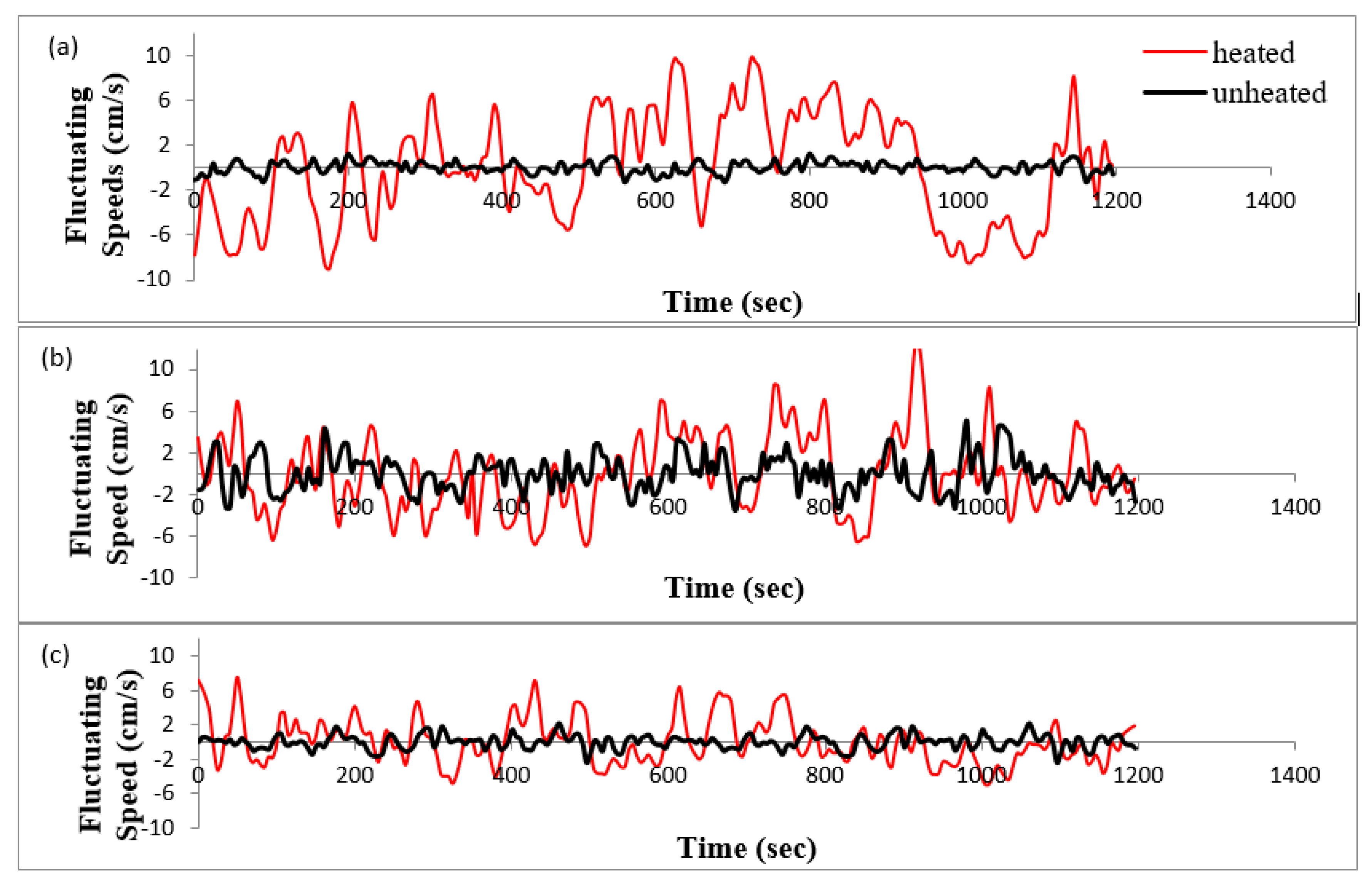
Sample results for the airflow speed for both cases, heated and unheated, are presented in Figure 8a–c. The local speeds in the east, center and west sides are also presented along with 95% confidence intervals in Figure 9. With heated manikins, the middle rows in the east side had relatively higher air speeds than in the front rows, whereas, in the west side, the air experienced higher speeds in the back section of the cabin. These observations were changed with unheated manikins, where the speed was more uniform across the cabin except near the front and back walls. Thus, the heated environment showed higher fluctuations and higher speeds, which was shown in Figure 8a–c and in most seats in Figure 9. This was also reflected on the values of the turbulence kinetic energy “k” and turbulence intensities “TI” at the different locations inside the cabin. The average values based on Equations (4) and (8) for k and TI, respectively, are shown in Figure 10 for k and in Figure 11 for TI. The values in Figure 9, Figure 10 and Figure 11 also included 95% confidence intervals.
The relative change between heated and unheated results for the turbulence kinetic energy and turbulence intensity were evaluated using Equation (11) and plotted in Figure 12 and Figure 13, respectively:
R e l a t i v e _ C h a n g e =   H e a t e d   U n h e a t e d   H e a t e d .
The relative change would serve as a quick indicator to which case had higher values. A positive value means that the heated results were higher than the unheated ones and vice versa. Out of 33 comparison locations in the east, center and west sides of the cabin, the heated cases showed a majority of higher values (27 points higher in both k and TI). There were two negative peaks for k and four negative peaks in TI comparisons that had relative change lower than 0.5. Relative change values for k showed that 22 seats (66% of the seats) had values between 0.5–1. This indicated the significant effect of thermal plumes or the heat generated by the manikins on the kinetic energy behavior inside the cabin. On the other side, for turbulence intensity, most of the values were between 0–0.5, which indicated warmer environments increased the turbulence intensity levels, but the effect was not as much as for turbulent kinetic energies. In general, the TI in the east and west sides of the cabin were less sensitive to heat than the turbulence kinetic energies were.
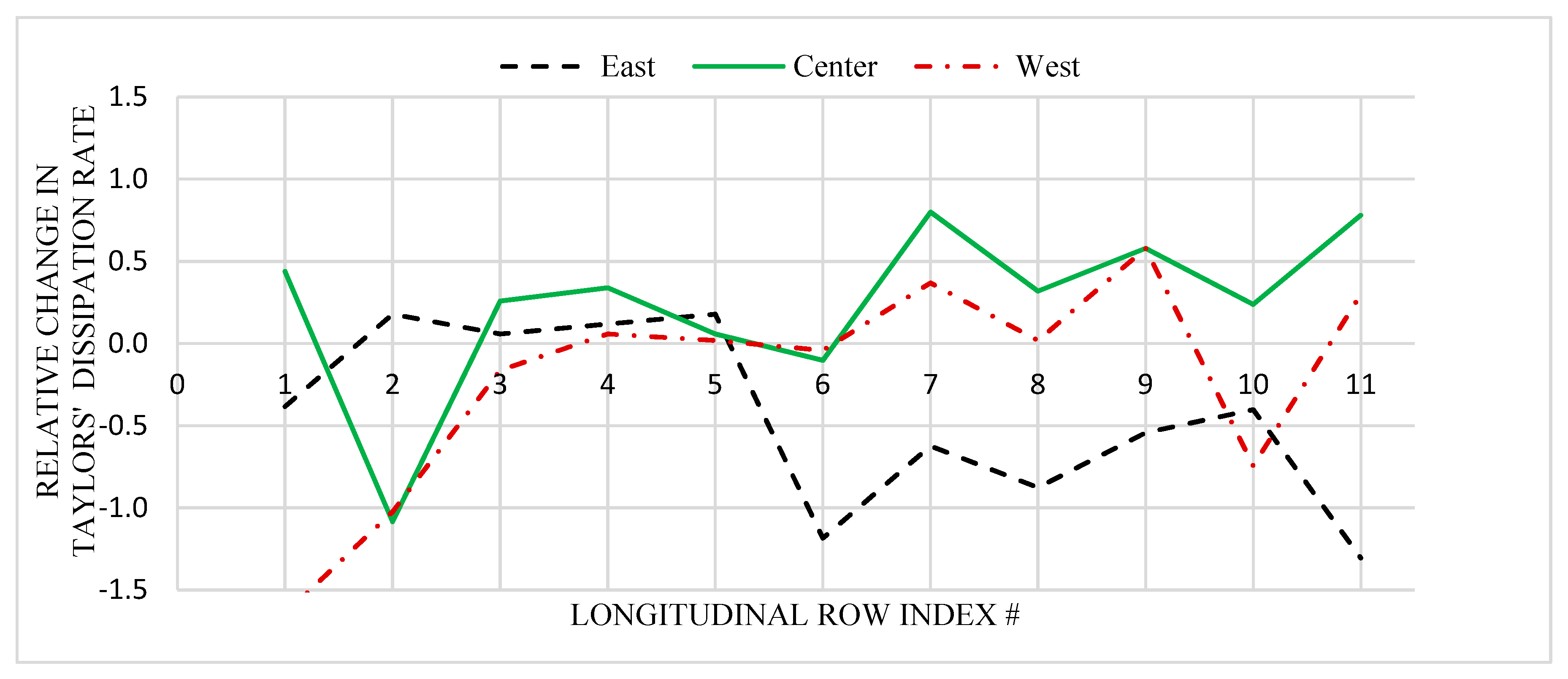
The change in k is related to the heat dissipated in each location. The discretized heat dissipation for heated and unheated cabins were evaluated using three transducers separated by a distance of 12.7 cm and utilizing Equation (9). The relative change in the dissipation rates with unheated manikins over heated cases were calculated using Equation (11) and the results are shown in Figure 14. Negative values would favor unheated results over heated ones or would mean the unheated cabin dissipated more energy than the heated ones and vice versa for positive values. As can be seen in Figure 14, the dissipation rates were higher for the unheated case in the front-west and back-east sides of the cabin. This indicated that the velocities and k were lower in these regions.

5. Uncertainty Analysis

For either the tracer gas measurements, TI, k or ε , the relative uncertainty contained two parts. The first one was the uncertainty due to measurement error “urandom” and the second one was due to the bias in the analyzer itself “ubias”. The total uncertainty was estimated using Equation (12):
u t o t a l =   ( u b i a s ) 2 +   ( u r a n d o m ) 2 .
The bias and random uncertainties for tracer gas measurements are given in Equations (13) and (14), respectively, where N is the number of samples collected, t95% is the 95% confidence interval constant and was estimated approximately 1.96, σ is the standard deviation of the samples collected, C ¯ n is the average normalized CO2 concentration in each location as indicated, and u c a b i n ,   u i n l e t ,   u e x i t are the relative uncertainty obtained by each analyzer. The uncertainty for each analyzer also included the uncertainty of the tracer gas used, repeatability of each analyzer, linearity of the measurements and uncertainty of the DAQ system used:
( u g a s , b i a s ) 2 =   [ C ¯ c a b i n C ¯ n ( C ¯ e x i t C ¯ i n l e t ) u c a b i n ] 2 + [ C ¯ e x i t ( C ¯ c a b i n C ¯ i n l e t ) C ¯ n ( C ¯ e x i t C ¯ i n l e t ) 2 u e x i t ] 2 +   [ C ¯ i n l e t ( C ¯ c a b i n C ¯ e x i t ) C ¯ n ( C ¯ e x i t C ¯ i n l e t ) 2 u i n l e t ] 2 ,
u g a s , r a n d o m =   t 95 % . σ n N 1 . C ¯ n .
Similarly, the random and bias uncertainties for k, TI and ε were calculated as given in Equations (15) through (20), where U v , b i a s   is the total bias uncertainty for the omni-directional TSI transducer (approximately 1% V ¯ ) , < > is the average of the reading (k, TI, or ε ), ( v , V   ¯ ,   v ) are the instantaneous, averaged and fluctuating components of the measured speed, and σ is the standard deviation of the variable:
u k , r a n d o m =   t 95 % . σ T K E N 1 . k , r e a d i n g s ,
u k , b i a s 2 =   8 ( U v , b i a s v ) 2 ,
u T I , r a n d o m =   t 95 % . σ T I N 1 T I , r e a d i n g s ,
( u T I , b i a s ) 2 =   ( U v , b i a s v ) 2 [ 1 +   ( v V ¯ ) 2 ]   ,
u ε , r a n d o m =   t 95 % . σ ε N 1 . ε ,
u ε , b i a s =   2 . u t r a n s d u c e r .
The relative uncertainty for all tracer gas sampling procedures ranged between ±5–14% for heated manikins versus ±8–17% for unheated manikins. For turbulence measurements, the relative uncertainties for heated and unheated environments, respectively, were ±14–39% and ±14–28% for the turbulence kinetic energy “k” and between ±11–34% and ±13–40% for dissipation rate analysis. For TI, the relative uncertainty was almost the same for both heated and unheated cases and ranged between ±7–11%. Thus, heated cases had higher uncertainties associated with k, whereas, with unheated cases, the normalized tracer gas concentrations and the dissipation rates were accompanied with higher uncertainties. This was expected due to the highly chaotic nature of the airflow inside the cabin.

6. Conclusions

An experimental study was conducted to check on the dispersion of tracer gas inside a Boeing aircraft model B767 cabin mockup made up of 11 rows with seven seats in the transverse direction of each row. The sampled tracer gas in the cabin was normalized against the inlet and outlet concentrations into and out of the cabin. Results for both manikins’ statuses, heated and unheated, were compared against each other. Testing with heated minikins showed multiple air circulations, which agreed with smoke visualization testing done by [19]. The multiple circulations were controlled by the minimum allowed distance inside the cabin, which was the height from the floor to the ceiling. The identified circulations in the rear section of the cabin were of comparatively smaller size than in other sections. The unheated tracer gas results showed more uniform tracer gas distribution around the release point.
Speed measurement showed smaller fluctuations with lower temperature environments indie the cabin. Hence, the turbulence kinetic energy values were higher with heated manikins testing than with unheated ones. This was the case as well with turbulence intensity, except that the difference between heated and unheated results were smaller than for turbulence kinetic energy. Regions inside the cabin that had lower turbulence kinetic energy level were accompanied with higher dissipation rates, which indicated that kinetic energy has been significantly dissipated as compared to heated regions. Thus, heated cases had higher uncertainties when evaluating “k”, whereas, with unheated cases, the normalized tracer gas concentrations and the dissipation rate estimations were accompanied with higher uncertainties. This was expected due to the highly chaotic nature of the airflow inside the cabin.
In conclusion, the air temperature inside the cabin can play an important role in affecting the air flow distribution and turbulence levels due to changes in convective heat and transport phenomena of the air.

Funding

The results presented are from research funded, in part, by the U.S. Federal Aviation Administration (FAA) Office of Aerospace Medicine through the National Air Transportation Center of Excellence for Research in the Intermodal Transport Environment under Cooperative Agreement 07-C-RITE-KSU. Although the FAA supported this project, it neither endorses nor rejects the findings of this research. The presentation of this information is in the interest of invoking technical community comment on results and conclusions of the research.

Conflicts of Interest

The author declares no conflict of interest.

References

  1. Lebbin, P.A.; Hosni, M.H.; Jones, B.W.; Beck, B.T.; Lin, C.H.; Horstman, R.H. Comparison of SPIV Measurements for Different Test Room Air Inlet Configurations with the Same Inlet Reynolds Number. ASHRAE Trans. 2006, 112, 54–59. [Google Scholar]
  2. Lin, C.; Wu, T.; Horstman, R.; Lebbin, P.; Hosni, M.; Jones, B.W.; Beck, B. Comparison of large eddy simulation predictions with particle image velocimetry data for the airflow in a generic cabin model. In Proceedings of the 10th International Conference on Indoor Air Quality and Climate, Beijing, China, 4–9 September 2005; Tsinghua University Press: Beijing, China, 2005. [Google Scholar]
  3. Ebrahimi, K.; Zheng, Z.; Hosni, M. LES and RANS Simulation of Turbulent Airflow and Tracer Gas Injection in a Generic Aircraft Cabin Model. In Proceedings of the ASME 2010 Fluids Engineering Division Summer Meeting, Montreal, BC, Canada, 1–5 August 2010; ASME: New York, NY, USA, 2010; pp. 227–240. [Google Scholar] [CrossRef]
  4. Ebrahimi, K.; Hosni, M.; Zheng, Z. Computational Study of Turbulent Airflow in a Full-Scale Aircraft Cabin Mockup—Part 1: Determination of Boundary Conditions at the Outlet of Air Diffusers. In Proceedings of the ASME 2013 Fluids Engineering Division Summer Meeting, Village, NV, USA, 7–11 July 2013; ASME: New York, NY, USA, 2013. [Google Scholar] [CrossRef]
  5. Anderson, M.; Jones, B.W.; Hosni, M. Impact of Personal Air Outlets on Person-to-Person Bio-Effluent Exposure in Aircraft Cabins. ASHRAE Trans. 2013, 119, 1–8, DE-13-C054. [Google Scholar]
  6. Patel, J.; Jones, B.; Hosni, M.; Keshavarz, A. Experimental investigation of ventilation effectiveness in an airliner cabin mockup. In Proceedings of the ASME 2016 International Mechanical Engineering Congress and Exposition, Phoenix, AZ, USA, 11–17 November 2016; ASME: New York, NY, USA, 2016. [Google Scholar] [CrossRef]
  7. Patel, J.; Jones, B.W.; Hosni, M. Experimental Analysis of Ventilation Effectiveness and Tracer Gas Dispersion in a Boeing-737 Mockup Cabin. In Proceedings of the Second International Conference on Energy and Indoor Environment for Hot Climates, Doha, Qatar, 26–27 February 2017; ASHRAE: Atlant, GA, USA, 2017. [Google Scholar]
  8. Shehadi, M. Experimental Investigation of Optimal Particulate Sensor Location inside an Aircraft Cabin. Master’s Thesis, Kansas State University, Manhattan, KS, USA, 2010. [Google Scholar]
  9. Kayser, C. General Features of the Problems of Aviation Toxicology, Aviation Toxicology: An Introduction to the Subject and a Handbook of Data; Committee on Aviation Toxicology, Aero Medical Association; The Blakiston Company: New York, NY, USA, 1953.
  10. Shehadi, M.; Hosni, M.; Jones, B.W. Airflow distribution in the longitudinal plan of a Boeing 767 mockup cabin. In Proceedings of the ASME 2014 International Mechanical Engineering Congress & Exposition, IMECE2014-40102, Montreal, QC, Canada, 14–20 November 2014. [Google Scholar]
  11. NRC. The Airliner Cabin Environment and the Health of Passengers and Crew; The National Academy Press: Washington, DC, USA, 2002.
  12. Shehadi, M.; Hosni, M.; Jones, B. Characterization of the frequency and nature of bleed air contamination events in commercial aircraft. Indoor Air 2016, 25, 478–488. [Google Scholar] [CrossRef] [PubMed]
  13. Launder, B.E.; Spalding, D.R. The numerical computation of turbulent flows. Comp. Meth. Appl. Mech. Eng. 1974, 3, 269–289. [Google Scholar] [CrossRef]
  14. Glasgow, L. Transport Phenomena—An Introduction to Advanced Topics; John Wiley and Sons: Hoboken, NJ, USA, 2010. [Google Scholar]
  15. ASHRAE: 2017 ASHRAE Handbook-Fundamentals; American Society for Heating, Refrigeration and Air-conditioning Engineers, Inc.: Atlanta, GA, USA, 2017.
  16. ASHRAE. ANSI/ASHRAE Standard 62-2001, Ventilation for Acceptable Indoor Air Quality; American Society of Heating, Refrigerating and Air-Conditioning Engineers, Inc.: Atlanta, GA, USA, 2001. [Google Scholar]
  17. O’Donnel, A.; Donnini, G.; Nguyen, V.H. Air quality, ventilation, temperature and humidity in aircraft. ASHRAE J. 1991, 4, 42–46. [Google Scholar]
  18. Beneke, J.M.; Jones, B.W.; Hosni, M.H. Fine Particle Dispersion in a Commercial Aircraft Cabin. HVAC&R Res. 2011, 17, 107–117. [Google Scholar]
  19. Shehadi, M.; Jones, B.; Hosni, B. Airflow and turbulence analysis inside a wide-body aircraft cabin mockup. Indoor Built Environ. 2018, 27, 766–785. [Google Scholar] [CrossRef]
Figure 1. Cabin mockup (a) exterior; (b) heating and cooling loops; and (c) interior of the cabin showing the thermally heated manikins.
Fluids 04 00167 g001
Figure 2. (a) tracer gas release tube; (b) tracer gas sampling tree.
Fluids 04 00167 g002aFluids 04 00167 g002b
Figure 3. Airflow prediction based on smoke visualization testing [13] and tracer gas release locations used.
Fluids 04 00167 g003
Figure 4. 8475 series TSI speed transducer.
Fluids 04 00167 g004
Figure 5. Results for airflow in the cabin with heated manikins [19].
Fluids 04 00167 g005
Figure 6. (a) normalized CO2 results for release in seat 2D (1 being at the front side of the cabin)—Heated case; (b) normalized CO2 results for release in seat 2D (1 being at the front side of the cabin)—Unheated case.
Fluids 04 00167 g006
Figure 7. (a) normalized CO2 results for release in seat 7D—Heated case; (b) normalized CO2 results for release in seat 7D—Unheated case.
Fluids 04 00167 g007
Figure 8. Comparison of the fluctuating speed in seat (a) 9D; (b) 7D; and (c) 6D with heated and unheated manikins.
Fluids 04 00167 g008
Figure 9. Comparison of the speed with heated and unheated manikins in east, centerline, and west side seats.
Fluids 04 00167 g009
Figure 10. Turbulence kinetic energy comparison for heated and unheated cases in the east, center and west sides of the cabin.
Fluids 04 00167 g010
Figure 11. Turbulence intensity comparisons for heated and unheated cases in the east, center and west sides of the cabin.
Fluids 04 00167 g011
Figure 12. Relative change in k between heated and unheated manikins.
Fluids 04 00167 g012
Figure 13. Relative change in TI between heated and unheated manikins.
Fluids 04 00167 g013
Figure 14. Dissipation rate relative change between heated and unheated cases.
Fluids 04 00167 g014
Table 1. Vertical normalized tracer gas comparison with heated and unheated cases.
Location Above FloorEast AisleWest Aisle
HeatedUnheatedHeatedUnheated
Release in Seat 2DRow 21792 mm16.5%41%51%34%
1344 mm17%36%70.0%35.5%
896 mm16%30%91%52%
448 mm23%39%99%74%
Release in Seat 5DRow 41792 mm29%20%13%19%
1344 mm33.5%26%16%19%
896 mm32%36%16%19%
448 mm37%46%20%29%
Row 61792 mm22%24%26%26%
1344 mm21.4%30%31%33%
896 mm23%35%33%30%
448 mm26%40%41%29%

