Linear Stability Analysis of Liquid Metal Flow in an Insulating Rectangular Duct under External Uniform Magnetic Field


Department of Aeronautics and Astronautics, Tokyo Metropolitan University, Hino, Tokyo 191-0065, Japan
Fluids 2019, 4(4), 177; https://doi.org/10.3390/fluids4040177
Submission received: 29 August 2019
/
Revised: 24 September 2019
/
Accepted: 27 September 2019
/
Published: 1 October 2019
(This article belongs to the Special Issue Numerical Analysis of Magnetohydrodynamic Flows)
Abstract
:Linear stability analysis of liquid metal flow driven by a constant pressure gradient in an insulating rectangular duct under an external uniform magnetic field was carried out. In the present analysis, since the Joule heating and induced magnetic field were neglected, the governing equations consisted of the continuity of mass, momentum equation, Ohm’s law, and conservation of electric charge. A set of linearized disturbance equations for the complex amplitude was decomposed into real and imaginary parts and solved numerically with a finite difference method using the highly simplified marker and cell (HSMAC) algorithm on a two-dimensional staggered mesh system. The difficulty of the complex eigenvalue problem was circumvented with a Newton—Raphson method during which its corresponding eigenfunction was simultaneously obtained by using an iterative procedure. The relation among the Reynolds number, the wavenumber, the growth rate, and the angular frequency was successfully obtained for a given value of the Hartmann number as well as for a direction of external uniform magnetic field.
1. Introduction
Magnetohydrodynamics is a discipline that deals with the interaction between electromagnetic fields and fluid flows, and its application encompasses a wide range of subjects, such as astrophysics, geodynamo phenomena, metallurgy, and electromagnetic pumps [1,2,3]. In magnetohydrodynamic flows, the most basic system is that a vertical uniform magnetic field is applied to the liquid metal flow between parallel plates, the so-called Hartmann flow, in which a sufficiently long container in the span direction is used [4,5]. The velocity distribution of the Hartmann flow is divided into a core region where viscosity is negligible and boundary layers formed near the wall perpendicular to the imposed magnetic field. This boundary layer is called the Hartmann boundary layer, but in a system with a finite span length, there is another boundary layer that develops near the walls parallel to the magnetic field, which was recently called the Shercliff boundary layer. The thickness of the Hartmann boundary layer is known to be proportional to the inverse of the Hartmann number.
The velocity distribution of the liquid metal flow, whether it is a parallel flow or a non-parallel flow with a temperature distribution like a natural convection flow, is influenced not only by the magnetic field strength and its direction but also by the electric conductivity of the container wall. When considering magnetohydrodynamics in mathematical formulas, one of the major points is whether to consider the induced magnetic field or not. This judgment is determined by the value of the magnetic Reynolds number. Since the magnetic Reynolds number is a dimensionless number given by the product of the magnetic Prandtl number and the Reynolds number, in general, the induced magnetic field cannot be ignored in high-speed flows or in the phenomena imposed by high-frequency magnetic fields [6]. However, in most cases of static magnetic field application, the induced magnetic field is often negligible. In this paper, the influence of the induced magnetic field is ignored.
In various industrial processes, such as semiconductor single crystal manufacturing, steel continuous casting processes, or fusion reactor blankets, the flow of liquid metal must be controlled to improve the quality of the final product. It is also necessary to understand the heat transfer of liquid metal under a magnetic field. In order to contribute to this point of view, theoretical, experimental, and numerical studies have been conducted thus far, but the thermal flow phenomenon in such high-temperature industrial processes is not easily handled experimentally. In addition, it is not easy to simulate the cases with respect to high Reynolds number (or Rayleigh number), low Prandtl number, and high Hartmann number. On the other hand, regarding the transition from laminar to turbulent flow, one of the theoretical approaches focusing on flow periodicity is the stability analysis of magnetohydrodynamic flows by Chandrasekar [7]. Hereafter, we refer to such research as follows.
The critical Reynolds number of the plane Poiseuille flow is known to be 5772 when the wave number takes 1.02. It is known that, when the Reynolds number exceeds that critical value, two-dimensional disturbance called a Tollmien—Schlichting wave is amplified with the phase speed of this wave 0.264 at the critical point. Stuart [8] discussed the effect of a uniform magnetic field applied parallel to the basic flow, while Lock [9] demonstrated the effect of a uniform vertical magnetic field on a plane Poiseuille flow by linear stability analysis. The parallel magnetic field does not affect the basic flow, but it affects the flow stability. On the other hand, the vertical magnetic field is characterized by the basic flow that itself is distorted under the influence of the magnetic field. In both cases, the flow tends to be stabilized by applying the uniform magnetic field. Takashima [10] carried out linear stability analysis for almost the same system as that by Lock [9], and he calculated critical values for various values of Hartmann number quite accurately with and without considering the effect of induced magnetic field.
Concerning the linear stability of parallel flow within a rectangular cross-section, Tatsumi and Yoshimura [11] and Adachi [12] are worth mentioning, although no magnetic field was applied in their configurations. Tatsumi and Yoshimura [11] reported the effect of the aspect ratio of the rectangular cross-section on the linear stability while paying attention to the fact that the Hagen—Poiseuille flow indicates linearly stable irrespective of the Reynolds number. When the aspect ratio of a cross-section becomes infinite, the value of critical Reynolds number approaches to that of the plane Poiseuille flow, while when the aspect ratio becomes smaller than a certain critical value (3.2), the linear stability analysis indicates that the critical Reynolds number is infinite as observed in the Hagen—Poiseuille flow. Concerning the mechanism of the discontinuous divergence of the critical Reynolds number to infinity in the vicinity of the critical aspect ratio around 3.2 reported by Tatsumi and Yoshimura [11], Adachi [12] found that the neutral curves consist of two bifurcation branches. One is the first bifurcation branch where the flow loses its stability with respect to three-dimensional disturbances, while the other is the second bifurcation branch where it recovers its stability.
Regarding the stability of parallel flow, it is known that there is a large discrepancy in critical values between the experiment and the linear theory, for instance, as indicated in the case of the Hagen—Poiseuille flow mentioned above. Airiau and Castets [13], Krasnov et al. [14], and Ksarnov et al. [15] made such a discussion in the case of magnetohydrodynamic flows. More recently, Dong et al. [16,17] obtained temporal growth and spatial distribution of perturbations based on nonmodal stability theory. It was also noted that the magnetohydrodynamic flow sometimes exhibited two-dimensional tendency in such situations that the main flow vorticity field and the external magnetic field were parallel to each other. In such cases, it was reported that the heat transfer coefficient of natural convection was enhanced by applying a uniform magnetic field [18,19,20]. Pothérat [21] performed linear stability analysis for a liquid metal within an insulating duct flow using the model from Sommeria and Moreau [22] where the flow field was assumed to be quasi-two-dimensional. More recently, Vo et al. [23] extended the investigation of Pothérat [21] by introducing vertical thermal stratification into the system, where the linear stability of Poiseuille—Rayleigh—Bénard flows under the effect of a transverse magnetic field was investigated.
The study of the effect of the magnetic field on the linear stability of parallel flow of liquid metal in a rectangular conducting duct can be found in the research from Priede, Bühler, and Molokov [24,25,26,27,28]. Among their studies, Hunt’s flow should be mentioned. In reference [24], the linear stability of the fully developed flow of a liquid metal in a square duct subject to a transverse magnetic field was studied numerically, but the walls of the duct perpendicular to the magnetic field were perfectly conducting, whereas the parallel ones were insulating. This case is called Hunt’s flow [29]. In a sufficiently strong magnetic field, the flow consists of two jets at the insulating walls and a near-stagnant core. Recently, Qi et al. [30] dealt with the case where the influence of buoyancy was incorporated together with Hunt’s flow. In these studies [24,25,26,27,28,29,30], the linear stability of the rather unstable flow with the inflection point of the basic flow was discussed. On the other hand, there have been no previous studies with three-dimensional numerical analysis on the stability of liquid metal flow in an insulating rectangular duct. Therefore, we carried out a linear stability analysis of liquid metal parallel flow in a duct with rectangular cross-section whose walls were electrically insulating. This configuration was similar to the recent study presented in a conference by Tagawa [31], and we extended this study in general, particularly focusing on the explanation of the numerical method.
2. Configuration of Problem and Governing Equations
We consider the magnetohydrodynamic parallel flow driven by a constant pressure gradient in a rectangular duct whose walls are electrically insulating. The primary flow is in Z-direction, and a uniform external magnetic field is imposed in either X- or Y-direction, as shown in Figure 1. In this study, we focus on a case where the aspect ratio of the cross-section of the duct is large enough that the basic flow is linearly unstable.
It is assumed that the fluid is an incompressible Newtonian fluid and the heat sources such as viscous dissipation and Joule heating are neglected. In addition to this, since the magnetic Prandtl number Prm is the order of 10−6 in most usual liquid metals, the induced magnetic field is neglected in this analysis. This study covers that the Reynolds number Re is less than the order of 105. The governing equations are written as follows.
Equation (1) is the continuity of mass, Equation (2) is the momentum balance, Equation (3) is the conservation of electric charge, Equation (4) is the Ohm’s law, and Equation (5) indicates the direction of external uniform magnetic field. Here, bx and by are constants. The boundary condition for velocity is no-slip and no-penetration at the four walls, and that for electric current density is electrically insulating, as shown in the boundary condition (6). Here, 2h is the height of the duct, and 2a is the spanwise length of the duct. It is noted that the characteristic length is h, which is the half length of the duct height in this study.
3. Basic State and Disturbance Equations
In the present analysis, we consider the case that the duct length along the primary flow is so long that a fully-established parallel flow is attained. Because of the parallel flow, the basic state having no disturbance is determined among the force balance between the pressure gradient, the viscous force, and the electromagnetic force. The solution of the basic state can be obtained by solving the following three equations numerically.
In this study, it is presumed that the maximum velocity of the plane Poiseuille flow is taken as the reference velocity uref, and the strength of the uniform applied magnetic field is taken as the reference magnetic field b0. The above equations are remade in a dimensionless form by using the following definitions.
The non-dimensional equations for the basic state are as follow.
In the analysis of parallel flow, the basic state is not related to the Reynolds number since there is no inertial term. The only relevant parameter in the present basic flow is the Hartmann number, whose square value represents the ratio of the Lorentz force to the viscous force. To examine the linear stability of the basic flow, the variables such as velocity, pressure, electric current density, and electric potential are assumed to be the sum of the basic state and the infinitesimal disturbance.
By substituting Equation (14) into Equations (1)–(4) and then neglecting quadric disturbances, the following linearized disturbance equations are obtained.
By considering the sinusoidal periodicity along the streamwise direction, infinitesimal disturbance is assumed to be given in the following form.
where k is the streamwise wavenumber (real number), and s is the complex number whose real part and imaginary part indicate the linear growth rate and the angular frequency, respectively. If > 0 for a certain wavenumber, its disturbance grows, and the basic flow is unstable, while if < 0 for all the wavenumbers, the disturbance attenuates, and the basic flow is stable. After substituting Equation (20) into Equations (15)–(19) and creating non-dimensionalization, the dimensionless disturbance equations for the complex amplitude are obtained.
The dimensionless variables and non-dimensional numbers are defined as follows.
Where Re represents the Reynolds number, Ha is the Hartmann number, A is the aspect ratio, α is the dimensionless wavenumber, and S is the dimensionless complex angular frequency. The system of the above equations and the boundary condition constitutes a generalized eigenvalue problem.
4. Numerical Methodology
As illustrated in Figure 2, the simultaneous partial differential equations for both the basic and the disturbance states were discretized on a two-dimensional equidistant staggered mesh system within a cross-section of the duct and solved with a finite difference method using the fourth-order central difference method. The discretization on a one-dimensional staggered mesh system with the cylindrical coordinate system can be found in our recent study in [32].
First, the variables of the basic state, such as streamwise velocity, electric current density, and electric potential, were obtained for a given Hartmann number. Then, the disturbance equations were numerically solved, during which both the linear growth rate and the angular frequency of the most unstable mode had to be determined for a given condition of parameters, such as wavenumber and Reynolds number. To circumvent such a complex eigenvalue problem, we employed a Newton—Raphson method. In Appendix A, the second-order central difference method is used to explain the computational algorithm for the eigenvalue problem in more detail.
5. Results and Discussion
5.1. Validation of the Code Diveloped
First of all, it was necessary to check the validity of the present numerical code. Our developed code is a two-dimensional one with the effect of electromagnetic force and can predict any neutral points for given parameters as the eigenvalue problems. Here, we checked the results of neutral values for the onset of instability in the plane Poiseuille flow without considering the effect of electromagnetic field. The obtained values for the neutral Reynolds number, the angular frequency, and the phase speed are summarized in Table 1 together with the dependency of grid resolution when the wavenumber 1.0205474 is given. The relative error in the Reynolds number becomes one order smaller as the number of meshes is doubled. It was judged that the present code can obtain quite accurate values when the number of meshes is sufficient.
Figure 3 shows the instantaneous profile of the velocity vectors and the pressure at the onset of instability, where the contribution of basic state is excluded from this profile. One wavelength is visualized because this unstable mode of travelling wave has periodicity along the streamwise direction. The color contour lines indicate that the perturbed pressure takes a positive value at the places where the perturbed velocity is positive. This tendency for the pressure can be easily understood by the fact that this perturbed velocity profile is superimposed with the basic flow, and the total flow exhibits a sinusoidal wavy profile. It is noted that the absolute value of the perturbed pressure is not important in the present linear analysis but is shown herein to display the numerical symmetry.
5.2. Hartmann Flow
When the aspect ratio of the cross-section becomes infinite with BX = 1 and BY = 0, the set of basic Equations (11)–(13) and that of disturbance Equations (21)–(27) are reduced to a set of ordinary differential equations.
Equation (29) shows the analytical solution for the Hartmann flow, and its velocity profile is visualized in Figure 4 for several values of the Hartmann number [1]. In this study, however, the basic flow profile is numerically obtained by solving Equation (28) instead of using Equation (29). Note that the spanwise velocity and the electric potential are zero, although the basic electric field E, which is induced in Y-direction, is non-zero constant.
Table 2 shows the summary of the critical values for several values of Hartmann number together with those obtained by Takashima [10]. The present computational results were checked by changing the two different mesh-systems. The critical Reynolds number monotonously increases as the Hartmann number increases. On the contrary, the wavenumber is not much varied, even though the Hartmann number changes. This tendency is consistent with the results by Lock [9] or Takashima [10], who used a Reynolds number based on the maximum velocity of the basic flow at each case of the Hartmann number. The Reynolds number defined by them is modified by the following relation in order to compare with the present results.
As the Hartmann number increases, compared with the results obtained by Takashima, the influence of mesh-dependency is rather obvious in the present study. This is due to the fact that the boundary layer thickness becomes thinner as the critical Reynolds number increases. For higher values of Ha > 5, the present computation is not impossible, but it is rather difficult to keep its numerical accuracy. In addition to this, neglecting the induced magnetic field is no longer valid since the critical Reynolds number at Ha = 7 is the order of 106, where the magnetic Reynolds number becomes the order of unity and therefore the induced magnetic field cannot be negligible.
Figure 5 shows the contour lines of the X-directional component of velocity for three cases of the Hartmann number. The red and the blue vortices indicate upward and downward velocity, respectively. As the Hartmann number increases, boundary layers formed in the vicinity of the two walls, which become thinner due to the increase in the critical Reynolds number. The profile of the contour lines is similar to the stream function Ψ because the following equation for is used to visualize the contour maps.
The stream function can be easily obtained by integrating Z, and it is almost equivalent to the imaginary part of . Therefore, the profile of the X-directional component of velocity is similar to that of stream function . This fact is also confirmed by comparing between Figure 3 and Figure 5.
Figure 6 shows the neutral stability curves of the Hartmann flow in the vicinity of the critical point for Ha = 1. For the range of wavenumber α > 1.05, the basic flow at Ha = 1 is always stable. The red symbols indicate the relation of Reynolds number and wavenumber, while the blue symbols indicate that of angular frequency and wave number. The value of the critical Reynolds number is approximately 10,840 when both wavenumber 0.972 and angular frequency 0.212 are given. As shown in Figure 6, the critical point is located at the upper curve of the angular frequency. Therefore, the lower curve of the angular frequency corresponds to the upper curve of the Reynolds number.
5.3. Finite Aspect Ratio
When the spanwise length of the duct is finite, it is necessary to take the sidewall effect into account. Since all duct walls are assumed to be electrically insulating, the effect of electric potential is crucial. In this study, the aspect ratio of spanwise length to duct height is limited to 5. Table 3 shows the summary of the computational results of the critical values obtained for relatively small Hartmann numbers. When no magnetic field is applied, the critical Reynolds number for A = 5 is much larger than that for the two-dimensional plane Poiseuille flow. According to Tatsumi and Yoshimura [11] or Adachi [12], it is reported that the critical Reynolds number for linear stability significantly depends on the aspect ratio of the duct cross-section. The critical values of the Reynolds number and the wavenumber for A = 5 are approximately 10,400 and 0.91, respectively. The critical Reynolds number by the present computation is not in agreement with Tatsumi and Yoshimura [11]. This may be due to the lack of grid resolution. The critical Reynolds number by the present code tends to produce smaller values than the previous studies, such as in Takashima [10] for the Hartmann flow and in Tatsumi and Yoshimura [11] for the duct flow of A = 5.
As the Hartmann number increases, the critical wavenumber αc tends to decrease slightly, but the Reynolds number increases rapidly. The X-directional magnetic field exhibits a better stabilizing effect than the Y-directional magnetic field provided the same Hartmann number is applied. In order to check the other magnetic field direction, Table 3 also includes results where the uniform magnetic field is applied obliquely at the angle of 45°. The reason that the stabilizing effect in the X-directional magnetic field is stronger than that in the Y-directional magnetic field is rather difficult to explain, but it is related to the configuration between the magnetic field direction and the axis of vortex in the flow. In the X-directional magnetic field, the magnetic field line and the axis of the vortex are perpendicular to each other, as already shown in the Hartmann flow. In this case, the streamwise component of velocity tends to be damped. In the Y-directional magnetic field, the magnetic field line and the axis of the vortex are parallel to each other. In this case, when the magnetic field becomes quite large, a quasi-two-dimensional flow that has little variation of the velocity profile [18,19,20,21,22] is observed.
It is noted that the accuracy of the computational results for the finite aspect ratio might be less than that for the Hartmann flow because of the requirement of two-dimensional meshing in the cross-sectional area as well as the high value of the critical Reynolds number. Therefore, in this subsection, we focus on the difference in flow characteristics affected by the direction of magnetic field rather than a quantitative discussion on the accurate critical values.
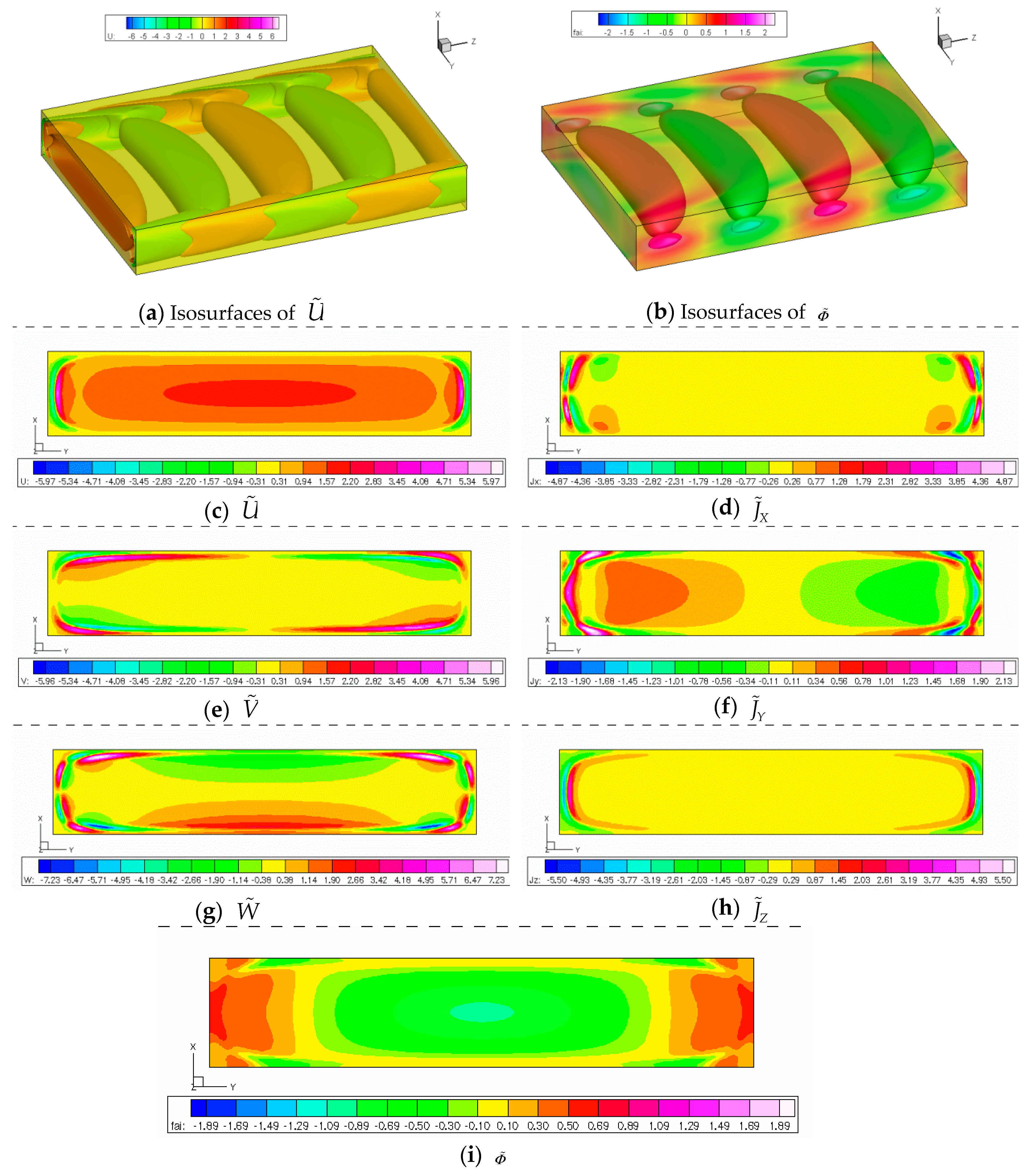
Figure 7 and Figure 8 show perspective views of the iso-surface of vertical velocity and electric potential , respectively, as well as cross-sectional views of the contour map for the three components of velocity, the three components of electric current density, and the electric potential when the uniform magnetic field is applied in either X-direction or Y-direction. Since the strength of the magnetic field is rather weak (Ha = 1), the velocity profiles seem almost similar to each other for both cases. However, the difference in electric current density and electric potential can be found, especially for the contour map of and . This can be explained by considering Ohm’s law, as shown in Equation (26). Since the symmetry mode of is (o,o) irrespective of the magnetic field direction, that of and in the X-directional magnetic field is also (o,o). In a similar way, the symmetry mode of is (e,e) irrespective of the magnetic field direction, and that of and in the Y-directional magnetic field is also (e,e). As shown in Figure 8b, the iso-surface of the electric potential is similar to that of the vertical component of velocity, as was explained using Equation (34), because the distribution of electric potential is quite similar to that of stream function when the magnetic field is applied in the direction parallel to the axis of vortices.
Table 4 summarizes the comparison for the symmetry modes between the X-directional and the Y-directional magnetic fields. There are no differences in the three components of velocity and pressure between the two magnetic fields, but the symmetry mode difference in electric current density and electric potential is found depending on the direction of the magnetic field. The modes of velocity and pressure fields were classified by Tasumi and Yoshimura [11] into four modes, I, II, III, and IV. The present result in the Y-directional magnetic field is equivalent to that obtained by Priede et al. [24] for mode I, where the uniform magnetic field is applied parallel to the conducting walls and perpendicular to the insulating walls.
6. Conclusions
Linear stability analysis of liquid metal flow driven by a constant pressure gradient in a rectangular duct under external uniform magnetic field applied either in the X- or the Y-direction was carried out. In this study, the liquid metal was assumed to be an incompressible Newtonian fluid, and the viscous dissipation, the Joule heating, and the induced magnetic field were neglected. A set of linearized disturbance equations for the complex amplitude was discretized on a two-dimensional staggered mesh system and solved with the use of the HSMAC (highly simplified marker and cell) method. The difficulty of the generalized eigenvalue problem was circumvented with the employment of a Newton—Raphson method.
Concerning the validation of the present code, one-dimensional computations were carried out for the plane Poiseuille flow in which neither meshing in the spanwise direction nor consideration of the effect of magnetic field were first attempted. As the number of meshes increased, both the Reynolds number and the angular frequency tended to coincide with the exact value.
When the aspect ratio of the cross-section of the rectangular duct was infinite, the set of disturbance equations could be drastically reduced without directly using electric current density. In the stability analysis of this Hartmann flow, the effect of insulating sidewalls was taken into account, but the flow near the sidewalls was neglected. The one-dimensional computation based on the present reduced equations suggested that the flow was stabilized as the Hartmann number increased. This result qualitatively agreed with the previous reports by Lock [9] and Takashima [10].
For the case that the aspect ratio of the cross-section of rectangular duct was five, both the basic flow and the disturbance equations were solved within a cross-sectional area. By comparing the symmetry modes between the X-directional and the Y-directional magnetic fields, the symmetry mode difference in electric current density and electric potential was found depending on the direction of magnetic field. The X-directional (vertical direction) magnetic field had a stronger effect than the Y-directional (spanwise direction) magnetic field on stabilization of liquid metal flow.
Author Contributions
Conceptualization, T.T.; methodology, T.T.; software, T.T.; validation, T.T.; formal analysis, T.T.; investigation, T.T.; resources, T.T.; data curation, T.T.; writing—original draft preparation, T.T.; writing—review and editing, T.T.; visualization, T.T.
Funding
This research received no external funding.
Conflicts of Interest
The authors declare no conflict of interest.
Nomenclature
| a | half spanwise length of duct (m) |
| A | aspect ratio = a/h (-) |
| b | magnetic flux density = (bx, by, 0) (T) |
| B | dimensionless magnetic flux density = b/ b0 = (BX, BY, 0) (-) |
| b0 | strength of external magnetic flux density = (bx2+ by2)1/2 (T) |
| C | coefficient of Newton—Raphson method |
| E | Electric field (V/m) |
| ex | unit vector in x direction (-) |
| ey | unit vector in y direction (-) |
| h | half length of duct height (m) |
| Ha | Hartmann number = b0h (σ/μ)1/2 (-) |
| i | imaginary unit (-) |
| j | electric current density = (jx, jy, jz) (A/m2) |
| J | dimensionless electric current density = (JX, JY, JZ) (-) |
| k | wavenumber in streamwise direction (rad/m) |
| p | pressure (Pa) |
| P | dimensionless pressure (-) |
| Prm | magnetic Prandtl number = σμmν = ν/νm (-) |
| Re | Reynolds number = uref h/ν (-) |
| Rem | magnetic Reynolds number = uref h/νm = PrmRe (-) |
| s | complex angular frequency = sr + isi (rad/s) |
| S | dimensionless complex angular frequency = SR + iSI (-) |
| SI | dimensionless angular frequency (-) |
| SR | dimensionless linear growth rate (-) |
| t | time (s) |
| u | x-directional velocity component (m/s) |
| u | velocity vector = (u, v, w) (m/s) |
| uref | reference velocity (m/s) |
| U | dimensionless x-directional velocity component = u/uref (-) |
| v | y-directional velocity component (m/s) |
| V | dimensionless y-directional velocity component = v/uref (-) |
| w | z-directional velocity component (m/s) |
| W | dimensionless z-directional velocity component = w/uref (-) |
| z | z coordinate (m) |
| Z | dimensionless z coordinate = z/h (-) |
| Greek symbols | |
| α | dimensionless wavenumber = kh (-) |
| μ | viscosity (Pa·s) |
| μm | magnetic permeability (H/m) |
| ν | kinematic viscosity = μ/ρ (m2/s) |
| νm | magnetic viscosity = 1/(σμm) (m2/s) |
| ρ | density (kg/m3) |
| σ | electric conductivity (1/(Ω·m)) |
| τ | dimensionless time (-) |
| φ | electric potential (V) |
| Φ | dimensionless electric potential (-) |
| Ψ | dimensionless stream function (-) |
| Subscripts or superscripts | |
| arb | arbitrary point |
| int | interpolation |
| c | critical |
| I | imaginary part |
| R | real part |
| i,j | grid point |
| n | time step |
| m | number of iteration |
| * | predictive |
| perturbed | |
| – | basic |
| ~ | complex amplitude |
Appendix A
In this appendix, the novelty of the present computational method for the stability analysis of fluid flow is highlighted. In the present study, the HSMAC method was used for solving both the basic state and the disturbance equations. One of the advantages of the present analysis using the HSMAC method was to be able to obtain the information of the pressure (in contrast to the use of the Orr—Sommerfeld equation) as well as to extend this method to multi-dimensional problems quite easily even in cases with or without the electromagnetic field. The set of disturbance equations constituted a complex eigenvalue problem. In this study, the difficulty of the complex eigenvalue problem was circumvented with a Newton—Raphson method during which its corresponding eigenfunction was simultaneously obtained by using an iterative procedure. The novelty of this simple procedure, which may allow many researchers to treat eigenvalue problems without using commercial software, is explained in the appendix.
Appendix A.1. Basic State
The basic state is numerically solved by a finite difference method with an iterative procedure. In the momentum equation, a virtual time-derivative term is introduced, as shown in Equation (A1) in order to make use of the iterative procedure. This virtual time-derivative method is almost equivalent to the Jacobi method if the time increment Δτ is as large as possible.
Here, the subscript “int” indicates the value interpolated at the cell-center points because the electric current density is defined at the cell -interfaces. The electric current density in the momentum equation is obtained by the HSMAC method. At a time instance (n+1), Equation (A2) is used for getting predictive values of electric current density. Then, Equations (A3) and (A4) are simultaneously used iteratively until the values of electric potential and electric current density are sufficiently converged. This convergence criterion is related to the accuracy of Equation (12).
The subscript i,j indicates grid location, while the superscripts m and n indicate the iteration of corrections for the convergence of Equation (A3) and the virtual time step, respectively.
Appendix A.2. How to Solve the Eigenvalue Problem
Equations (21)–(26) are decomposed into the real and the imaginary parts, respectively, and the set of partial differential disturbance equations is discretized on the same staggered mesh system as used in the computation of the basic state. The time-derivative terms are also introduced in Equations (22), (23), and (24) in order to make use of the iterative procedure together with the HSMAC method. The most unstable mode can be automatically obtained by this procedure although its complex eigenvalue has to be acquired by some means. This is explained at the end of this subsection. After getting the predictive values of the three velocity components from Equations (22), (23), and (24), the pressure and the velocity components are simultaneously corrected by the following discretized Equations (A5) and (A6).
Since Equations (A5) and (A6) contain imaginary units, both the real and the imaginary components have to be solved simultaneously. In a similar way, after getting the predictive value of electric current density vector from Equation (26), the electric potential and the three components of electric current density are also corrected by the following discretized equations. It is noted that there is no time increment Δτ in Equations (A7) and (A8).
The complex eigenvalue for the most unstable mode can be obtained by using Equation (A10). For instance, Equation (22) is utilized at an arbitrary point during the stage of predictive computation, as shown in Equation (A9). Both the real and the imaginary parts are shown in Equation (A9).
where f (SR) is regarded as a function of SR only, although SI is also included, while f (SI) is regarded as a function of SI only although SR is also included. Owing to the formula of the Newton—Raphson method, the following equations are derived from the real and the imaginary parts of Equation (A9), respectively.
where CR and CI are constants and are responsible for each convergence speed. By adopting Equation (A10) during the stage of predictive computation, both the linear growth rate SR and the angular frequency SI are automatically obtained. Meanwhile, the eigenfunction of the most unstable mode should be normalized in order to set it uniquely. In this study, the value of a component of velocity at an arbitrary point within the staggered mesh system is fixed at unity during the computation.
Appendix A.3. How to Obtain Neutral Curve
For a given Ha, α and Re, the obtained eigenvalue SR (growth rate) is not zero. For the purpose of obtaining a neutral stability curve, it is desired to get a combination among Ha, α, Re, and SI that satisfies SR is equal to zero. Herein, the values of Ha and α are fixed, but Re is freely varied. The value of neutral Reynolds number Re is gradually modified so that SR approaches zero. During such an iterative procedure, the value of SI is also gradually modified. Equation (A11) is useful for getting a neutral Reynolds number.
where C1 is the positive constant, and its value is responsible for the convergence speed. For SR > 0, the value of Re becomes gradually smaller until SR = 0 is satisfied. For SR < 0, Re becomes gradually larger until the value of Re is converged. Figure A1 shows an example for neutral stability curve. The region inside the curve is unstable (SR > 0), and the infinitesimal disturbance grows, whereas the region outside the curve is stable (SR < 0). Therefore, by using Equation (A11), the lower branch of the curve can be obtained for a given wavenumber. If the sign of C1 is set to a negative value, the upper branch of the curve can be acquired for a given wavenumber. The part connecting the upper and the lower curves is very steep, and therefore it is difficult to seek the neutral Reynolds number. In such a situation, on the contrary, a neutral wavenumber is easily obtained when the Reynolds number is set as a given parameter.
Figure A1.
An example of neutral curve.

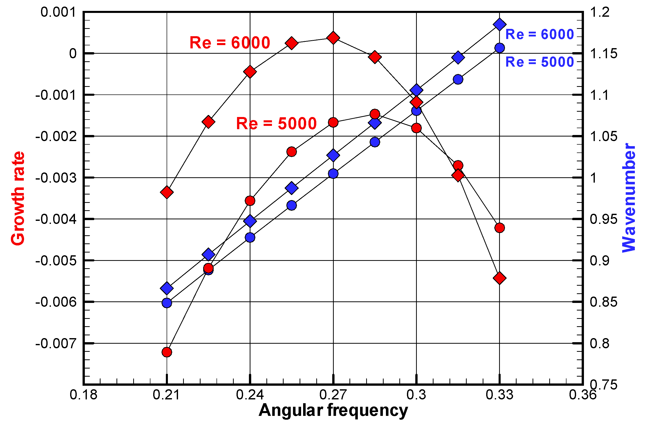
It is sometimes required to seek both α and SR for a given combination of Re and SI. Figure A2 depicts an exemplified result of the plane Poiseuille flow. The red symbols indicate the relation of growth rate and angular frequency, while the blue symbols indicate that of wavenumber and angular frequency. The blue symbols exhibit linear tendency for both Re = 5000 and 6000. To get this kind of figure, the following equation is utilized instead of Equation (A11).
where, C2 is the positive constant, and its value is responsible for the convergence speed, and ω is an input value of angular frequency. Equation (A12) converges if the value of SI becomes the same as that of ω. Meanwhile, Equation (A10) should always be applied.
Figure A2.
An example of relation among wavenumber, growth rate, and angular frequency for the plane Poiseuille flow for two different values of the Reynolds number (Re = 5000 and 6000).
Figure A2.
An example of relation among wavenumber, growth rate, and angular frequency for the plane Poiseuille flow for two different values of the Reynolds number (Re = 5000 and 6000).
Appendix A.4. How to Determine Critical Point
As shown in Figure A1, the critical Reynolds number does not change along the neutral curve at the point of critical wavenumber, i.e., the derivative of Re for α is zero at the critical point. From the Newton—Raphson method, the following formula is derived.
By the use of the second-order central difference method, the critical wavenumber that takes the minimum neutral Reynolds number is automatically obtained by using the following equation iteratively.
where Δα is the increment of wavenumber, which is an input parameter. and are the values of neutral Reynolds number at α and α ± Δα, respectively. The superscript m indicates the number of iterations.
References
- Moreau, R.J. Magnetohydrodynamics; Fluid Mechanics and Its Application; Kluwer Academic Publishers: Dordrecht, The Netherlands; Norwell, MA, USA, 1990; Volume 3. [Google Scholar]
- Ozoe, H. Magnetic Convection; Imperial College Press: London, UK, 2005. [Google Scholar]
- Molokov, S.; Moreau, R.; Moffatt, H.K. Magnetohydrodynamics: Historical Evolution and Trends; Fluid Mechanics and Its Application; Springer: Berlin/Heidelberg, Germany, 2007; Volume 80. [Google Scholar]
- Müller, U.; Bühler, L. Magnetofluiddynamics in Channels and Containers; Springer: Berlin/Heidelberg, Germany, 2001. [Google Scholar]
- Moreau, R.; Molokov, S. Julius Hartmann and his followers: A review on the properties of the Hartmann layer. In Magnetohydrodynamics; Springer: Berlin/Heidelberg, Germany, 2007; pp. 155–170. [Google Scholar]
- Ueno, K. Inertia effect in two-dimensional MHD channel flow under a traveling sine wave magnetic field. Phys. Fluids A Fluid Dyn. 1991, 3, 3107–3116. [Google Scholar] [CrossRef]
- Chandrasekhar, S. Hydrodynamic and Hydromagnetic Stability; Dover Publication: Mineola, NY, USA, 1961. [Google Scholar]
- Stuart, J.T. On the stability of viscous flow between parallel planes in the presence of a co-planar magnetic field. Proc. R. Soc. Lond. Series A Math. Phys. Sci. 1954, 221, 189–206. [Google Scholar] [CrossRef]
- Lock, R.C. The stability of the flow of an electrically conducting fluid between parallel planes under a transverse magnetic field. Proc. R. Soc. Lond. Series A Math. Phys. Sci. 1955, 233, 105–125. [Google Scholar] [CrossRef]
- Takashima, M. The stability of the modified plane Poiseuille flow in the presence of a transverse magnetic field. Fluid Dyn. Res. 1996, 17, 293. [Google Scholar] [CrossRef]
- Tatsumi, T.; Yoshimura, T. Stability of the laminar flow in a rectangular duct. J. Fluid Mech. 1990, 212, 437–449. [Google Scholar] [CrossRef]
- Adachi, T. Linear stability of flow in rectangular ducts in the vicinity of the critical aspect ratio. Eur. J. Mech. B Fluids 2013, 41, 163–168. [Google Scholar] [CrossRef]
- Airiau, C.; Castets, M. On the amplification of small disturbances in a channel flow with a normal magnetic field. Phys. Fluids 2004, 16, 2991–3005. [Google Scholar] [CrossRef]
- Krasnov, D.S.; Zienicke, E.; Zikanov, O.; Boeck, T.; Thess, A. Numerical study of the instability of the Hartmann layer. J. Fluid Mech. 2004, 504, 183–211. [Google Scholar] [CrossRef] [Green Version]
- Krasnov, D.; Zikanov, O.; Rossi, M.; Boeck, T. Optimal linear growth in magnetohydrodynamic duct flow. J. Fluid Mech. 2010, 653, 273–299. [Google Scholar] [CrossRef]
- Dong, S.; Liu, L.; Ye, X. Linear stability analysis of magnetohydrodynamic duct flows with perfectly conducting walls. PLoS ONE 2017, 12, e0186944. [Google Scholar] [CrossRef]
- Dong, S.; Liu, L.S.; Ye, X.M. Instability of MHD Flow in the Duct with Electrically Perfectly Conducting Walls. J. Appl. Fluid Mech. 2017, 10, 1293–1304. [Google Scholar] [CrossRef]
- Tagawa, T.; Ozoe, H. Enhancement of heat transfer rate by application of a static magnetic field during natural convection of liquid metal in a cube. J. Heat Transf. 1997, 119, 265–271. [Google Scholar] [CrossRef]
- Tagawa, T.; Ozoe, H. Enhanced heat transfer rate measured for natural convection in liquid gallium in a cubical enclosure under a static magnetic field. J. Heat Transf. 1998, 120, 1027–1032. [Google Scholar] [CrossRef]
- Authié, G.; Tagawa, T.; Moreau, R. Buoyant flow in long vertical enclosures in the presence of a strong horizontal magnetic field. Part 2. Finite enclosures. Eur. J. Mech. B Fluids 2003, 22, 203–220. [Google Scholar] [CrossRef]
- Pothérat, A. Quasi-two-dimensional perturbations in duct flows under transverse magnetic field. Phys. Fluids 2007, 19, 074104. [Google Scholar] [CrossRef]
- Sommeria, J.; Moreau, R. Why, how, and when, MHD turbulence becomes two-dimensional. J. Fluid Mech. 1982, 118, 507–518. [Google Scholar] [CrossRef]
- Vo, T.; Pothérat, A.; Sheard, G.J. Linear stability of horizontal, laminar fully developed, quasi-two-dimensional liquid metal duct flow under a transverse magnetic field and heated from below. Phys. Rev. Fluids 2017, 2, 033902. [Google Scholar] [CrossRef]
- Priede, J.; Aleksandrova, S.; Molokov, S. Linear stability of Hunt’s flow. J. Fluid Mech. 2010, 649, 115–134. [Google Scholar] [CrossRef]
- Priede, J.; Aleksandrova, S.; Molokov, S. Linear stability of magnetohydrodynamic flow in a perfectly conducting rectangular duct. J. Fluid Mech. 2012, 708, 111–127. [Google Scholar] [CrossRef] [Green Version]
- Priede, J.; Arlt, T.; Bühler, L. Linear stability of magnetohydrodynamic flow in a square duct with thin conducting walls. J. Fluid Mech. 2016, 788, 129–146. [Google Scholar] [CrossRef]
- Arlt, T.; Priede, J.; Bühler, L. The effect of finite-conductivity Hartmann walls on the linear stability of Hunt’s flow. J. Fluid Mech. 2017, 822, 880–891. [Google Scholar] [CrossRef]
- Bühler, L.; Arlt, T.; Boeck, T.; Braiden, L.; Chowdhury, V.; Krasnov, D.; Mistrangelo, C.; Molokov, S.; Priede, J. Magnetically induced instabilities in duct flows. In IOP Conference Series: Materials Science and Engineering; IOP Publishing: Bristol, UK, 2017; Volume 228, p. 012003. [Google Scholar]
- Hunt, J.C.R. Magnetohydrodynamic flow in rectangular ducts. J. Fluid Mech. 1965, 21, 577–590. [Google Scholar] [CrossRef]
- Qi, T.Y.; Liu, C.; Ni, M.J.; Yang, J.C. The linear stability of Hunt-Rayleigh-Bénard flow. Phys. Fluids 2017, 29, 064103. [Google Scholar] [CrossRef] [PubMed]
- Tagawa, T. Linear stability of parallel flow of liquid metal in a rectangular duct driven by a constant pressure gradient under the influence of a uniform magnetic field. In IOP Conference Series: Materials Science and Engineering; IOP Publishing: Bristol, UK, 2018; Volume 424, p. 012016. [Google Scholar]
- Tagawa, T.; Song, K. Stability of an axisymmetric liquid metal flow driven by multi-poles rotating magnetic field. Fluids 2019, 4, 77. [Google Scholar] [CrossRef]
Figure 1.
Sketch of the duct flow problem with uniform magnetic field imposed either in X- or Y-direction. All four side walls are electrically insulating.
Figure 1.
Sketch of the duct flow problem with uniform magnetic field imposed either in X- or Y-direction. All four side walls are electrically insulating.

Figure 2.
The equidistant staggered mesh system employed in the computations of basic and disturbance equations. The variables such as pressure and electric potential are defined at the cell-centers indicated with red points, while the vector components are defined at the cell-interfaces indicated with blue and green arrows.
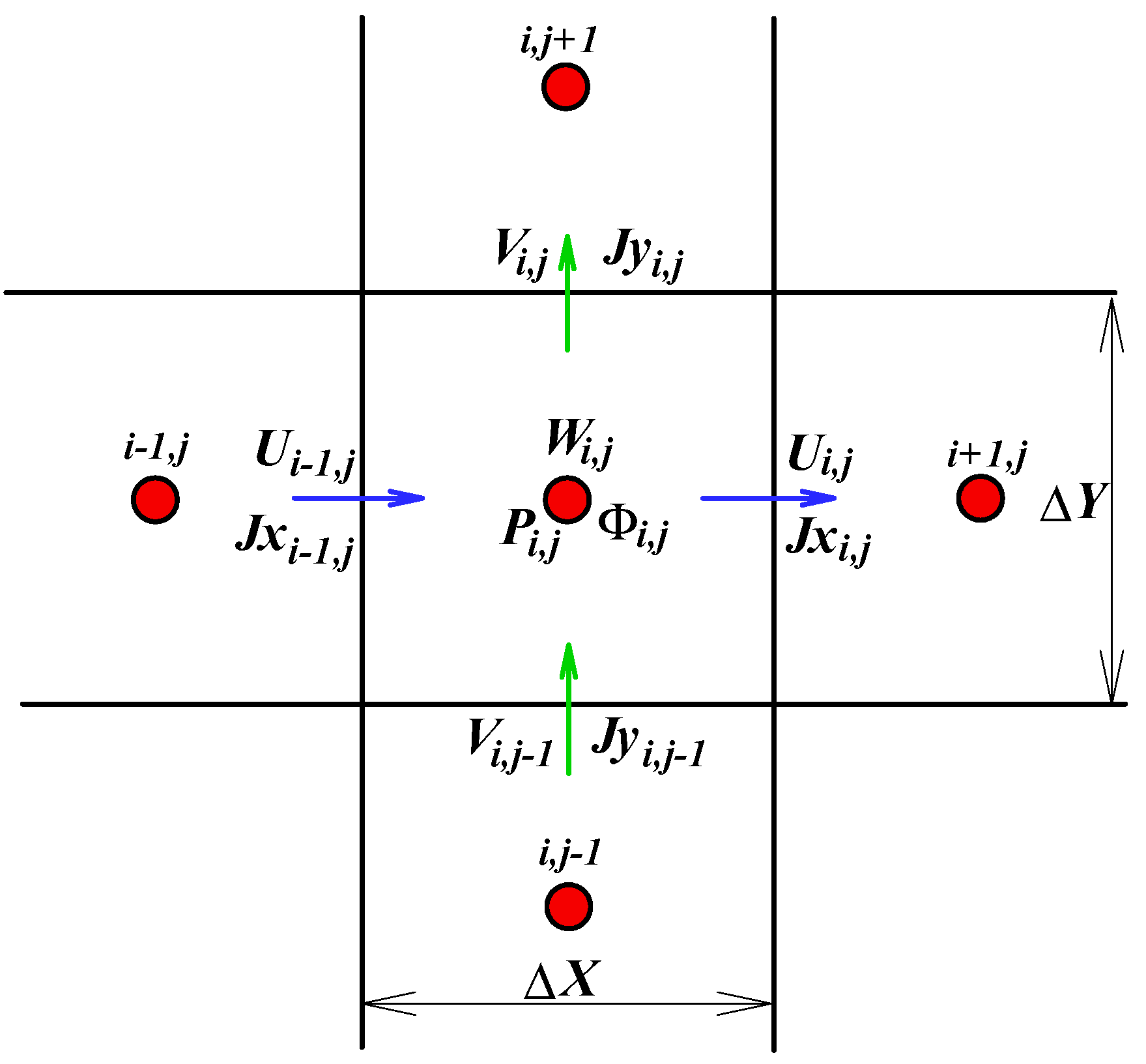
Figure 3.
Visualization of eigenfunctions of velocity vector and pressure for a wavelength at a critical point (Re = 5772, α = 1.02 and Cph = 0.264).
Figure 3.
Visualization of eigenfunctions of velocity vector and pressure for a wavelength at a critical point (Re = 5772, α = 1.02 and Cph = 0.264).
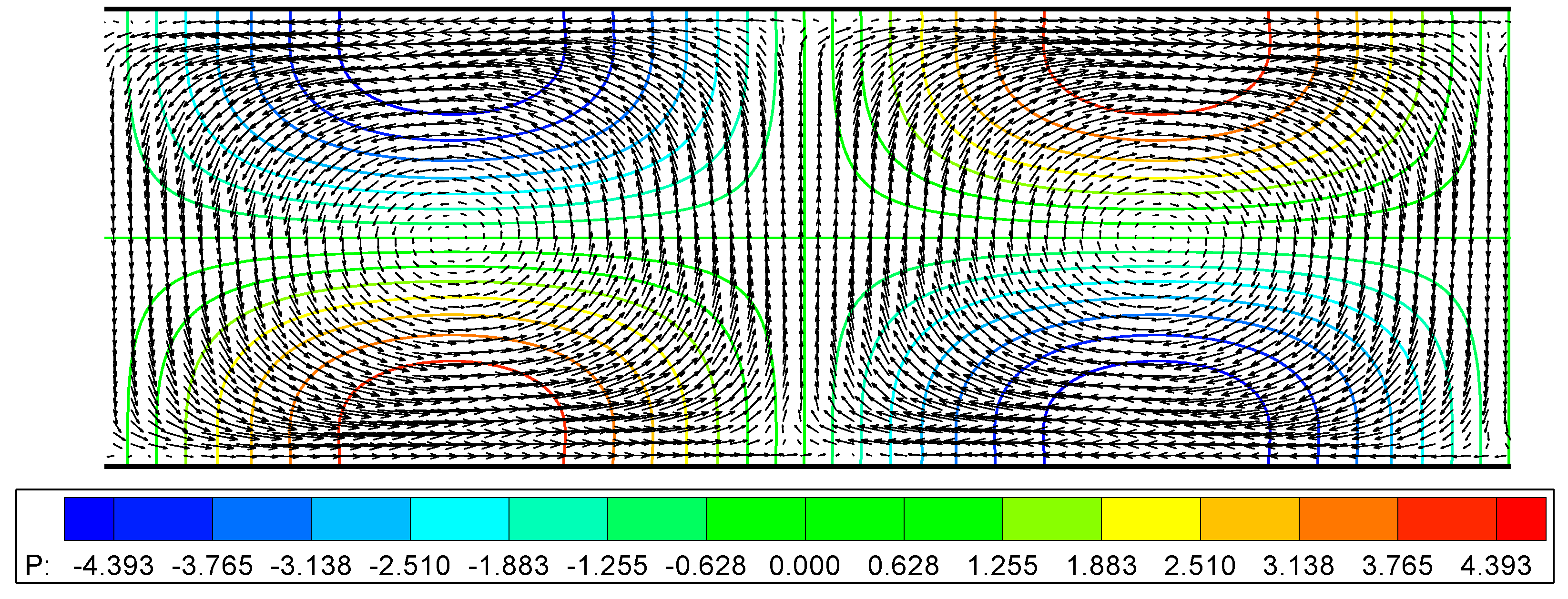
Figure 4.
Basic velocity profile of the Hartmann flow with insulating sidewalls for several values of Hartmann number.
Figure 4.
Basic velocity profile of the Hartmann flow with insulating sidewalls for several values of Hartmann number.
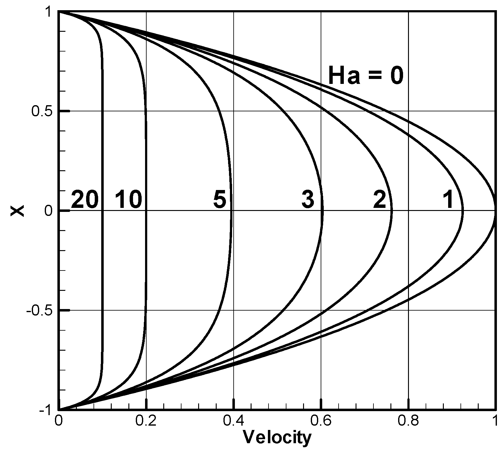
Figure 5.
The contour lines of the X-directional component of velocity at the critical state for Ha = 1, 3, and 5. The computational conditions of wavenumber, Reynolds number, and angular frequency are as listed in Table 2.
Figure 5.
The contour lines of the X-directional component of velocity at the critical state for Ha = 1, 3, and 5. The computational conditions of wavenumber, Reynolds number, and angular frequency are as listed in Table 2.
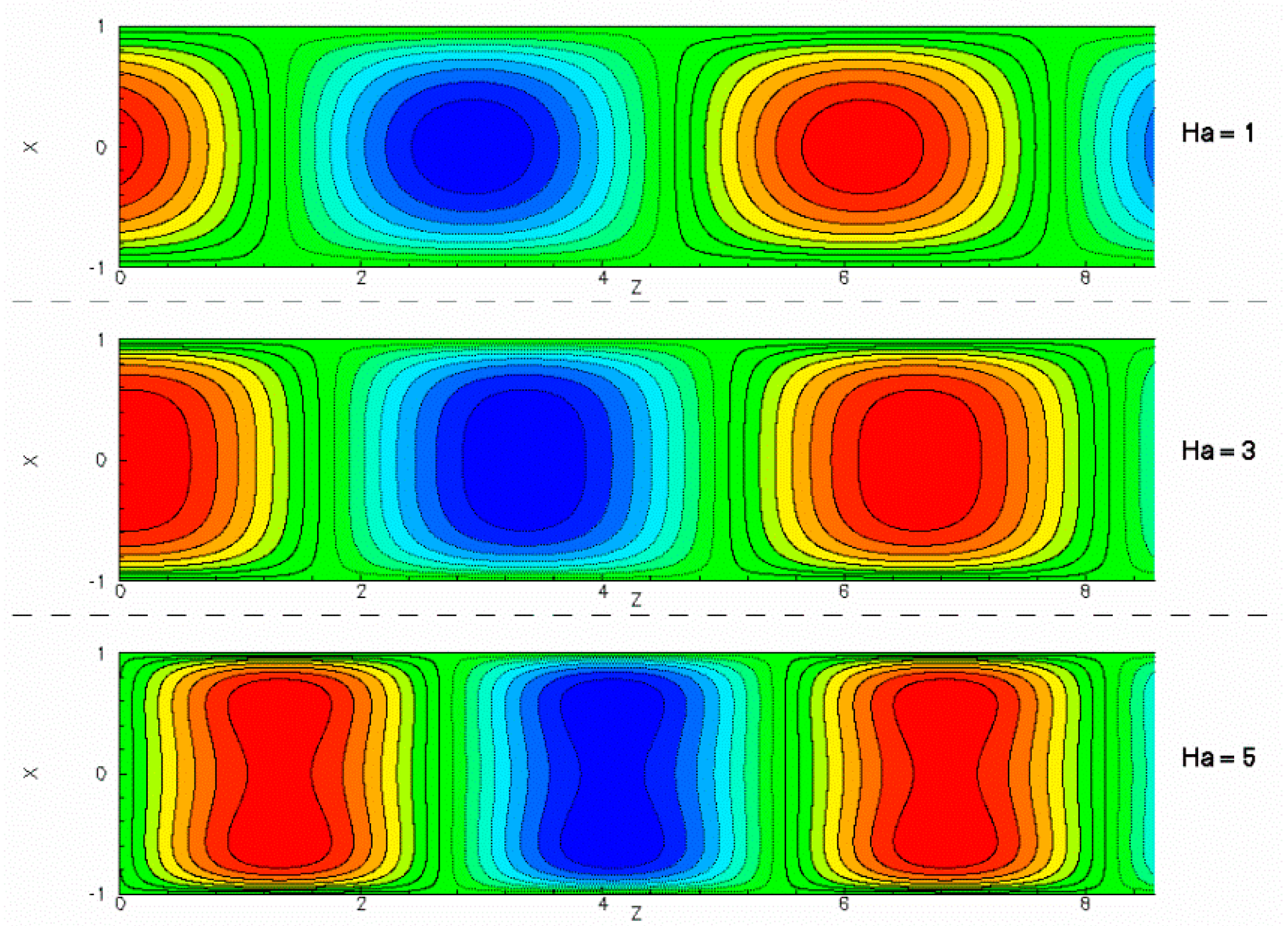
Figure 6.
Neutral stability curves in the vicinity of the critical point for Ha = 1.
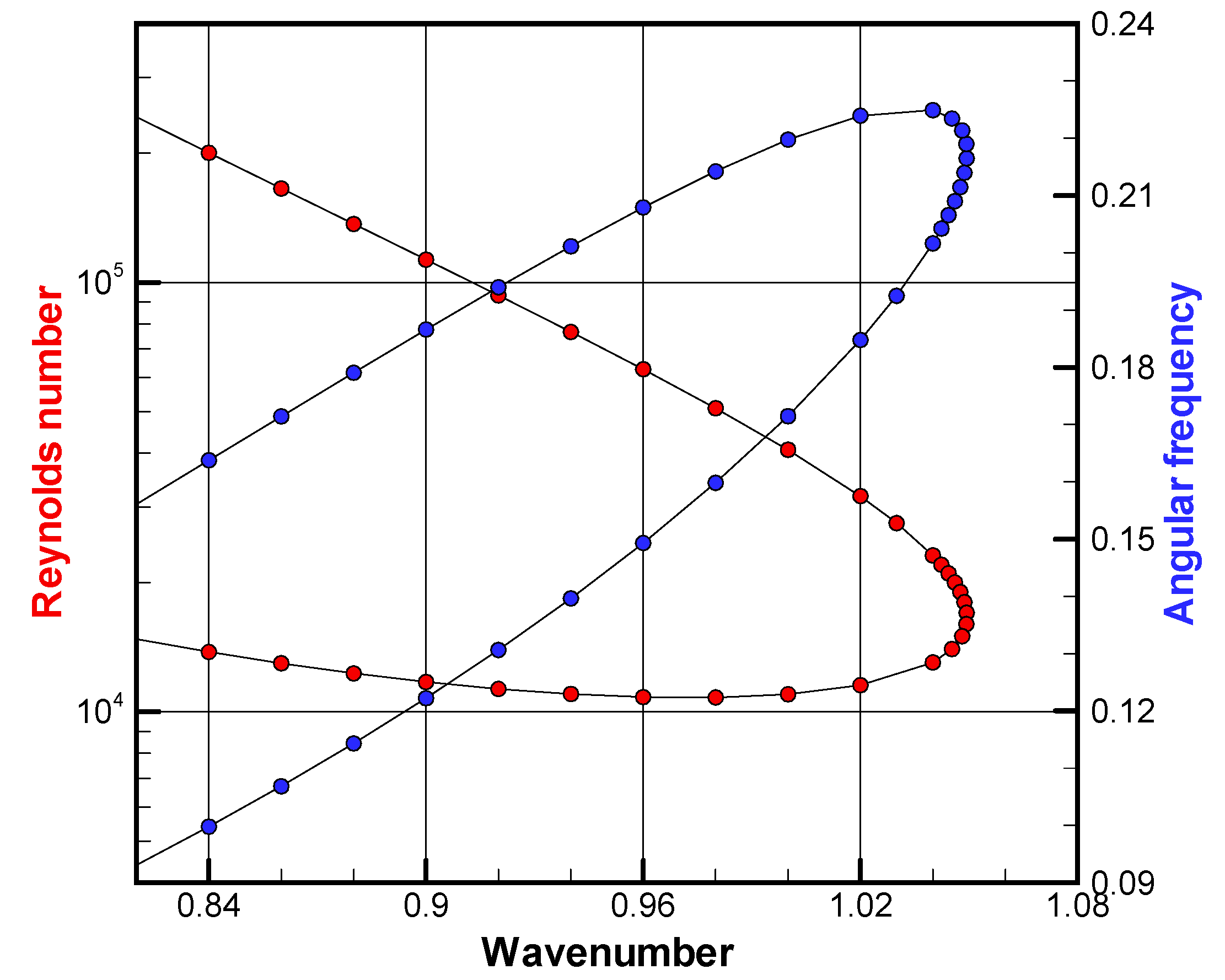
Figure 7.
Contour maps at the critical state when external uniform magnetic field is applied in X-direction (B = ex) at A = 5, Ha = 1, αc = 0.8737, Rec = 20,140, and SIc = −0.1680. (a) Iso-surface of vertical component of velocity; (b) iso-surface of electric potential; (c) contour map of ; (d) contour map of ; (e) contour map of ; (f) contour map of ; (g) contour map of ; (h) contour map of ; (i) contour map of

Figure 8.
Contour maps at the critical state when external uniform magnetic field is applied in Y-direction (B = ey) at A = 5, Ha = 1, αc = 0.9129, Rec = 10,933, and SIc = −0.2097. (a) Iso-surface of vertical component of velocity; (b) iso-surface of electric potential; (c) contour map of ; (d) contour map of ; (e) contour map of ; (f) contour map of ; (g) contour map of ; (h) contour map of ; (i) contour map of .

Table 1.
Dependency on number of meshes for the neutral value of Reynolds number, angular frequency, phase speed, and relative error in Reynolds number deviated from the exact value at α = 1.0205474 and SR = 0.
Table 1.
Dependency on number of meshes for the neutral value of Reynolds number, angular frequency, phase speed, and relative error in Reynolds number deviated from the exact value at α = 1.0205474 and SR = 0.
| Number of Meshes | Re | −SI | Cph | Error in Re |
|---|---|---|---|---|
| 100 | 5720.572 | 0.2699707 | 0.2645352 | 8.95 × 10⁻³ |
| 200 | 5767.318 | 0.2694774 | 0.2640518 | 8.50 × 10⁻⁴ |
| 400 | 5771.866 | 0.2694287 | 0.2640041 | 6.17 × 10⁻⁵ |
| 800 | 5772.198 | 0.2694250 | 0.2640005 | 4.16 × 10⁻⁶ |
| Exact value | 5772.222 | 0.2694248 | 0.2640003 | - |
Table 2.
Summary of the critical values obtained for several values of Hartmann number. Dependency on the number of meshes and the comparison with Takashima’s results are shown.
Table 2.
Summary of the critical values obtained for several values of Hartmann number. Dependency on the number of meshes and the comparison with Takashima’s results are shown.
| Present | Takashima [10] | ||||||
|---|---|---|---|---|---|---|---|
| Ha | Number of Meshes | αc | Rec | −SIc | αc | ReTak. | Remod |
| 0 | 200 | 1.0207 | 5767.31 | 2.695 × 10⁻¹ | 1.0205 | 5772.22 | 5772.22 |
| 400 | 1.0206 | 5771.87 | 2.694 × 10⁻¹ | ||||
| 1 | 200 | 0.9722 | 10,817.5 | 2.118 × 10⁻¹ | 0.9718 | 10,016.3 | 10837.4 |
| 400 | 0.9718 | 10,835.9 | 2.116 × 10⁻¹ | ||||
| 2 | 200 | 0.9294 | 37,274.3 | 1.363 × 10⁻¹ | 0.9277 | 28,603.6 | 37,577.5 |
| 400 | 0.9279 | 37,532.8 | 1.358 × 10⁻¹ | ||||
| 3 | 200 | 0.9636 | 105,614 | 9.901 × 10⁻² | 0.9582 | 65,155.2 | 107,974 |
| 400 | 0.9588 | 107,702 | 9.788 × 10⁻² | ||||
| 4 | 200 | 1.0476 | 224,231 | 8.180 × 10⁻² | 1.0354 | 112,395 | 233,178 |
| 400 | 1.0372 | 231,617 | 8.008 × 10⁻² | ||||
| 5 | 200 | 1.1527 | 399,687 | 7.230 × 10⁻² | 1.1342 | 164,090 | 415,791 |
| 400 | 1.1386 | 410,155 | 7.060 × 10⁻² | ||||
Table 3.
Effect of the direction of the uniform magnetic field on the critical values obtained for various values of Hartmann number at A = 5. The number of meshes employed within the cross-section is 50 × 250 in the X- and the Y-directions, respectively.
Table 3.
Effect of the direction of the uniform magnetic field on the critical values obtained for various values of Hartmann number at A = 5. The number of meshes employed within the cross-section is 50 × 250 in the X- and the Y-directions, respectively.
| Direction of Magnetic Field | Ha | αc | Rec | −SIc |
|---|---|---|---|---|
| - | 0 | 0.9255 | 9883.7 | 0.2193 |
| X | 0.5 | 0.9119 | 11,783 | 0.2051 |
| 1.0 | 0.8765 | 19,489 | 0.1700 | |
| 1.5 | 0.8797 | 36,013 | 0.1446 | |
| 2.0 | 1.0808 | 55,378 | 0.1711 | |
| Y | 0.5 | 0.9223 | 10,139 | 0.2169 |
| 1.0 | 0.9124 | 10,944 | 0.2098 | |
| 1.5 | 0.8952 | 12398 | 0.1983 | |
| 2.0 | 0.8710 | 14,582 | 0.1832 | |
| 2.5 | 0.8437 | 17,382 | 0.1672 | |
| 3.0 | 0.8214 | 20,570 | 0.1536 | |
| 3.5 | 0.8031 | 24367 | 0.1417 | |
| 4.0 | 0.8987 | 54,436 | 0.1518 | |
| XY | 1.0 | 0.8934 | 14,670 | 0.1884 |
| 2.0 | 0.8658 | 36,837 | 0.1414 |
Table 4.
The computational results obtained for the symmetry modes for the X-directional magnetic field and the Y-directional magnetic field. The notation is such that, e.g., (o,e) stands for an odd function in x-direction and an even function in y-direction.
Table 4.
The computational results obtained for the symmetry modes for the X-directional magnetic field and the Y-directional magnetic field. The notation is such that, e.g., (o,e) stands for an odd function in x-direction and an even function in y-direction.
| X-mag. (B = ex) | Y-mag. (B = ey) |
© 2019 by the author. Licensee MDPI, Basel, Switzerland. This article is an open access article distributed under the terms and conditions of the Creative Commons Attribution (CC BY) license (http://creativecommons.org/licenses/by/4.0/).
Share and Cite
MDPI and ACS Style
Tagawa, T. Linear Stability Analysis of Liquid Metal Flow in an Insulating Rectangular Duct under External Uniform Magnetic Field. Fluids 2019, 4, 177. https://doi.org/10.3390/fluids4040177
AMA Style
Tagawa T. Linear Stability Analysis of Liquid Metal Flow in an Insulating Rectangular Duct under External Uniform Magnetic Field. Fluids. 2019; 4(4):177. https://doi.org/10.3390/fluids4040177
Chicago/Turabian StyleTagawa, Toshio. 2019. "Linear Stability Analysis of Liquid Metal Flow in an Insulating Rectangular Duct under External Uniform Magnetic Field" Fluids 4, no. 4: 177. https://doi.org/10.3390/fluids4040177