Liquid-Cooling System of an Aircraft Compression Ignition Engine: A CFD Analysis

Abstract

The present work deals with an analysis of the cooling system for a two-stroke aircraft engine with compression ignition. This analysis is carried out by means of a 3D finite-volume RANS equations solver with k-$ϵ$ closure. Three different cooling system geometries are critically compared with a discussion on the capabilities and limitations of each technical solution. A first configuration of such a system is considered and analyzed by evaluating the pressure loss across the system as a function of the inlet mass-flow rate. Moreover, the velocity and vorticity patterns are analyzed to highlight the features of the flow structure. Thermal effects on the engine structure are also taken into account and the cooling system performance is assessed as a function of both the inlet mass-flow rate and the cylinder jackets temperatures. Then, by considering the main thermo-fluid dynamics features obtained in the case of the first configuration, two geometrical modifications are proposed to improve the efficiency of the system. As regards the first modification, the fluid intake is split in two manifolds by keeping the same total mass-flow rate. As regards the second configuration, a new single-inlet geometry is designed by inserting restrictions and enlargements within the cooling system to constrain the coolant flow through the cylinder jackets and by moving downstream the outflow section. It is shown that the second geometry modification achieves the best performances by improving the overall transferred heat of about 20% with respect to the first one, while keeping the three cylinders only slightly unevenly cooled. However, an increase of the flow characteristic loads occurs due to the geometrical restrictions and enlargements of the cooling system.

1. Introduction

It is well known that internal combustion engines for aeronautical applications operate within a specific temperature range to avoid structural damages, detonations and loss of efficiency of the combustion process. The heat released by combustion is only partially converted to work: a certain amount is within exhaust gases, while the remaining part warms-up the engine structure. This heat needs to be some how dissipated by keeping the engine within its optimal temperature range as to ensure reliability and long service life [1]. This temperature range (roughly from 350 to 380 K) ensures that the engine is efficiently working from the thermodynamic point of view. Indeed, a high cooling would reduce the engine thermal efficiency whereas if the engine temperature exceeds this range, the engine may over-heat and this over-heating is likely to damage the engine. The engine over-heating can be prevented by using efficient cooling systems to assist the engine running at its optimal performance. Hence, there is a need to look at the total heat balance and control system for the aircraft in order to search for performance optimization [2,3,4].

Generally, for piston aircraft engines, either air or liquid cooling systems are employed; only a few modern engines implement a combination of both, all with their own advantages and disadvantages [5]. Inline four, six or eight cylinders engines are almost exclusively air-cooled, except for the Rotax, Viking and Subaru engines and some aero diesels [6]. Such a cooling technique represents a good compromise between the structure design and the low weight achieved when compared to liquid cooling circuits. Nevertheless, air-cooled cylinders present a large number of fins cast around the heads increasing the total exposed surface. Indeed, the engine may be shock-cooled at high altitudes [7]. On the other hand, liquid-cooling systems have a weight penalty with respect to air-based systems while they are able to keep the temperature of all of the cylinders quite even and the engine cannot be shock-cooled during high speed or low power descends. Moreover, the coolant liquid is usually thermostatically controlled so that the engine is quickly warmed up at the start-up and works all the time around the optimal operating temperature [8].

In this context, a detailed analysis of such cooling systems is required by the designer to optimize the heat distribution of the engine structure. Computational Fluid Dynamics (CFD) simulations provide a means to optimize cooling circuit configurations by employing sensitivity analysis to the components of such circuits. Indeed, simulation models are very useful for engineers not only to support but also to reduce the amount of testing required during the design of the engine. Numerical models and simulations can greatly enhance development efforts by predicting performance trends and trade-offs and will, therefore, result in more efficient and better-optimized heating and cooling systems for high-performing engines [9,10,11,12,13,14]. Specifically, due to the wide spatial and temporal scales involved in internal combustion engine simulations, steady and unsteady Reynolds-averaged Navier–Stokes (RANS) solvers are largely employed supporting the rational design of such engines. Moreover, recently, hybrid approaches involving both unsteady RANS and Large Eddy Simulations (LES) techniques have also been proposed thus achieving the required resolutions needed for a comprehensive analysis of such engines [15,16,17].

In this work, a liquid cooling system for a specific aircraft engine is analyzed by means of a 3D finite-volume RANS equations solver with k-$ϵ$ closure. Specifically, the RANS equations for an incompressible thermal fluid is used to analyze the cooling system performance as a function of the inlet mass-flow rate G${}_{In}$. Such analysis is carried out by varying the cylinder jackets temperature and by comparing the outflow temperature and the transferred thermal power as a function of coolant mass-flow rate. The CFD results enable us to notice the drawbacks of the cooling system geometry and suggest some improvements that can be used to enhance the heat transfer. Two geometrical modifications to the cooling system are proposed. The first modification consists of two coolant inlets while keeping the same total mass-flow rate; the second configuration consists of a new single-inlet geometry with new restrictions and enlargements within the cooling system to constrain the coolant flow through the cylinder jackets and also by positioning downstream the outflow manifold. Capabilities and limitations of these three cooling system geometries are critically discussed and compared providing useful insights for the internal combustion engine community.

2. The Model

2.1. Mathematical Model

The steady three-dimensional Reynolds-Averaged Navier-Stokes (RANS) system of equations with the k–$ϵ$ closure reads:

$$\frac{\partial (E-E_v)}{\partial x}+\frac{\partial (F-F_v)}{\partial y}+\frac{\partial (G-G_v)}{\partial z}=S,$$

(1)

where E, F and G are the inviscid flux vectors:

$$E=\left(\begin{array}{c}\overline{u}\\ \rho {\overline{u}}^2+p_t\\ \rho \overline{u}\overline{v}\\ \rho \overline{u}\overline{w}\\ \rho c_p\overline{T}\overline{u}\\ \rho \overline{u}k\\ \rho \overline{u}ϵ\end{array}\right),F=\left(\begin{array}{c}\overline{v}\\ \rho \overline{u}\overline{v}\\ \rho {\overline{v}}^2+p_t\\ \rho \overline{v}\overline{w}\\ \rho c_p\overline{T}\overline{v}\\ \rho \overline{v}k\\ \rho \overline{v}ϵ\end{array}\right),G=\left(\begin{array}{c}\overline{w}\\ \rho \overline{u}\overline{w}\\ \rho \overline{v}\overline{w}\\ \rho {\overline{w}}^2+p_t\\ \rho c_p\overline{T}\overline{w}\\ \rho \overline{w}k\\ \rho \overline{w}ϵ\end{array}\right);$$

(2)

where overbar indicates Reynolds-averaging of the physical variable; $\rho$ is the density; $(\overline{u},\overline{v},\overline{w})$ and $\overline{T}$ are the Reynolds-averaged velocity components and temperature, respectively; ${\overline{p}}_t=\overline{p}+\frac{2}{3}k$ being $\overline{p}$ the Reynolds-averaged pressure; k and $ϵ$ are the turbulent kinetic energy and its dissipation rate.

$E_v$, $F_v$ and $G_v$ represent the viscous flux vectors, reading:

$$E_{\nu }=\left(\begin{array}{c}0\\ \mu \frac{\partial \overline{u}}{\partial x}\\ \mu \frac{\partial \overline{v}}{\partial x}\\ \mu \frac{\partial \overline{w}}{\partial x}\\ \lambda \frac{\partial \overline{T}}{\partial x}+\mu [2{(\frac{\partial \overline{u}}{\partial x})}^2+{(\frac{\partial \overline{v}}{\partial x}+\frac{\partial \overline{u}}{\partial y})}^2]\\ {\mu }_t\frac{\partial k}{\partial x}\\ {\mu }_t\frac{\partial ϵ}{\partial x}\end{array}\right),F_{\nu }=\left(\begin{array}{c}0\\ \mu \frac{\partial \overline{u}}{\partial y}\\ \mu \frac{\partial \overline{v}}{\partial y}\\ \mu \frac{\partial \overline{w}}{\partial y}\\ \lambda \frac{\partial \overline{T}}{\partial y}+\mu [2{(\frac{\partial \overline{v}}{\partial y})}^2+{(\frac{\partial \overline{w}}{\partial y}+\frac{\partial \overline{v}}{\partial z})}^2]\\ {\mu }_t\frac{\partial k}{\partial y}\\ {\mu }_t\frac{\partial ϵ}{\partial y}\end{array}\right),$$

$$G_{\nu }=\left(\begin{array}{c}0\\ \mu \frac{\partial \overline{u}}{\partial z}\\ \mu \frac{\partial \overline{v}}{\partial z}\\ \mu \frac{\partial \overline{w}}{\partial z}\\ \lambda \frac{\partial \overline{T}}{\partial z}+\mu [2{(\frac{\partial \overline{w}}{\partial z})}^2+{(\frac{\partial \overline{u}}{\partial z}+\frac{\partial \overline{w}}{\partial x})}^2]\\ {\mu }_t\frac{\partial k}{\partial z}\\ {\mu }_t\frac{\partial ϵ}{\partial z}\end{array}\right);$$

(3)

being $\mu$, ${\mu }_t$ and $\lambda$ the molecular viscosity, turbulent viscosity and thermal diffusivity, respectively. Finally, S corresponds to the source term vector,

$$S=\left(\begin{array}{c}0\\ 0\\ 0\\ 0\\ 0\\ S_k\\ S_{ϵ}\end{array}\right),$$

(4)

where $S_k$ and $S_{ϵ}$ are the source terms related to k and $ϵ$, respectively.

The steady-state RANS equations with k–$ϵ$ turbulence closure are solved by means of a cell-centered finite volume numerical scheme. The computational domain is discretized by a multi-block unstructured mesh. A pressure-based solver is employed where the equations are solved segregated one to each other, i.e., each equation is decoupled from all the others. Indeed, this segregated algorithm is memory-efficient, since the discretized equations need only to be located in the memory one at a time [18]. Specifically, the SIMPLE solver by Patankar and Spalding [19] is employed. Viscous terms are discretized by a second-order-accurate least-squares cell-centered scheme [20], while convective terms are treated with a second-order upwind scheme [21]. The pressure and velocity fields are solved by using a SIMPLE-type pressure-velocity coupling in which the momentum equation is solved using an estimated initial pressure field. Then, the SIMPLE correction for the pressure field is employed to satisfy the continuity equation. The pressure-correction equation is solved by using the algebraic multigrid (AMG) method by Hutchinson and Raithby [22]. In the present work, only steady flows are considered; therefore, the algorithm is iterated in a pseudo-time until a residual drop of at least four orders of magnitude for all of the conservation-law equations is achieved. No-slip conditions are imposed along the engine walls while the near-wall region of the flow field is treated with the standard wall-functions approach proposed by Launder and Spalding [23].

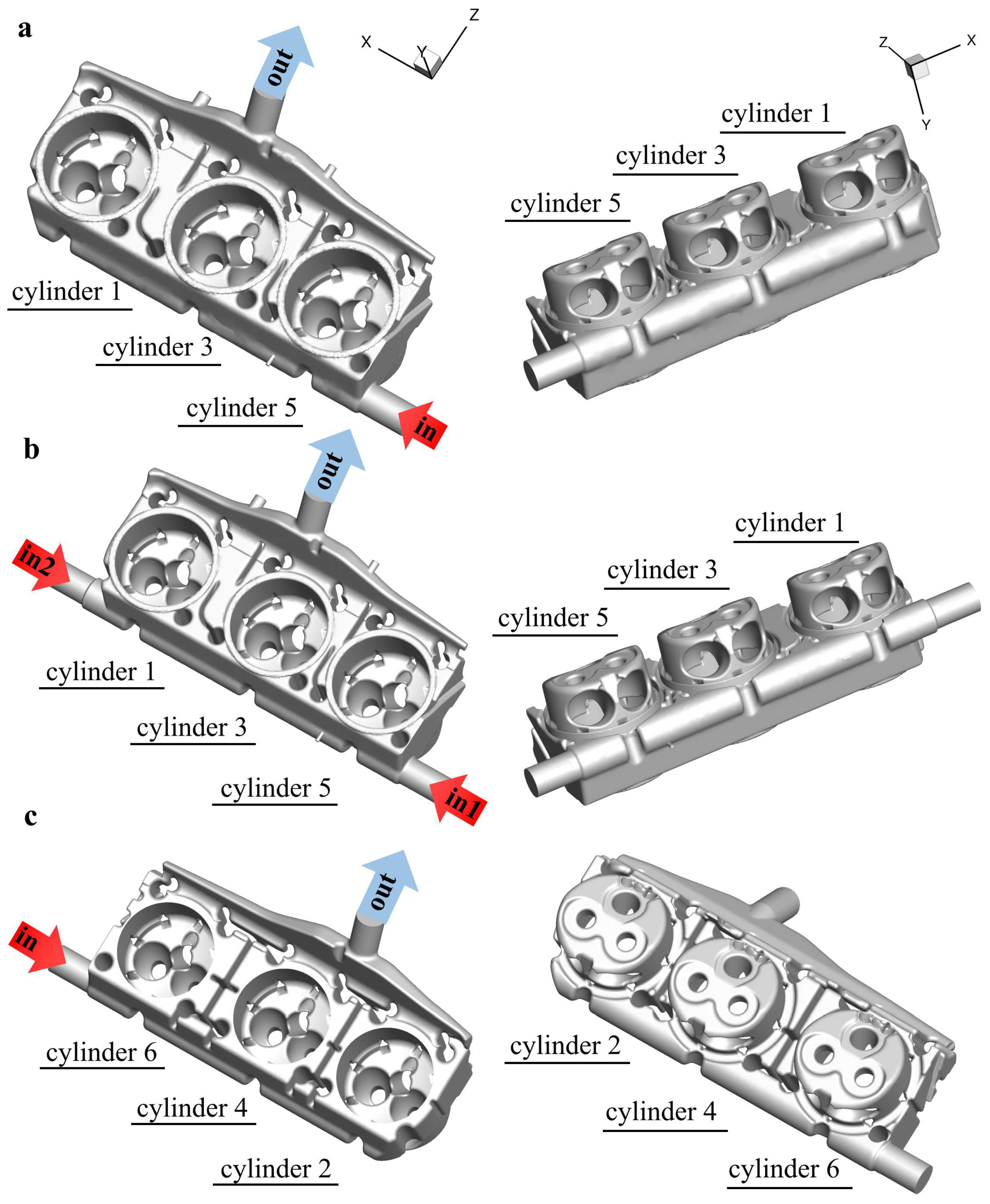
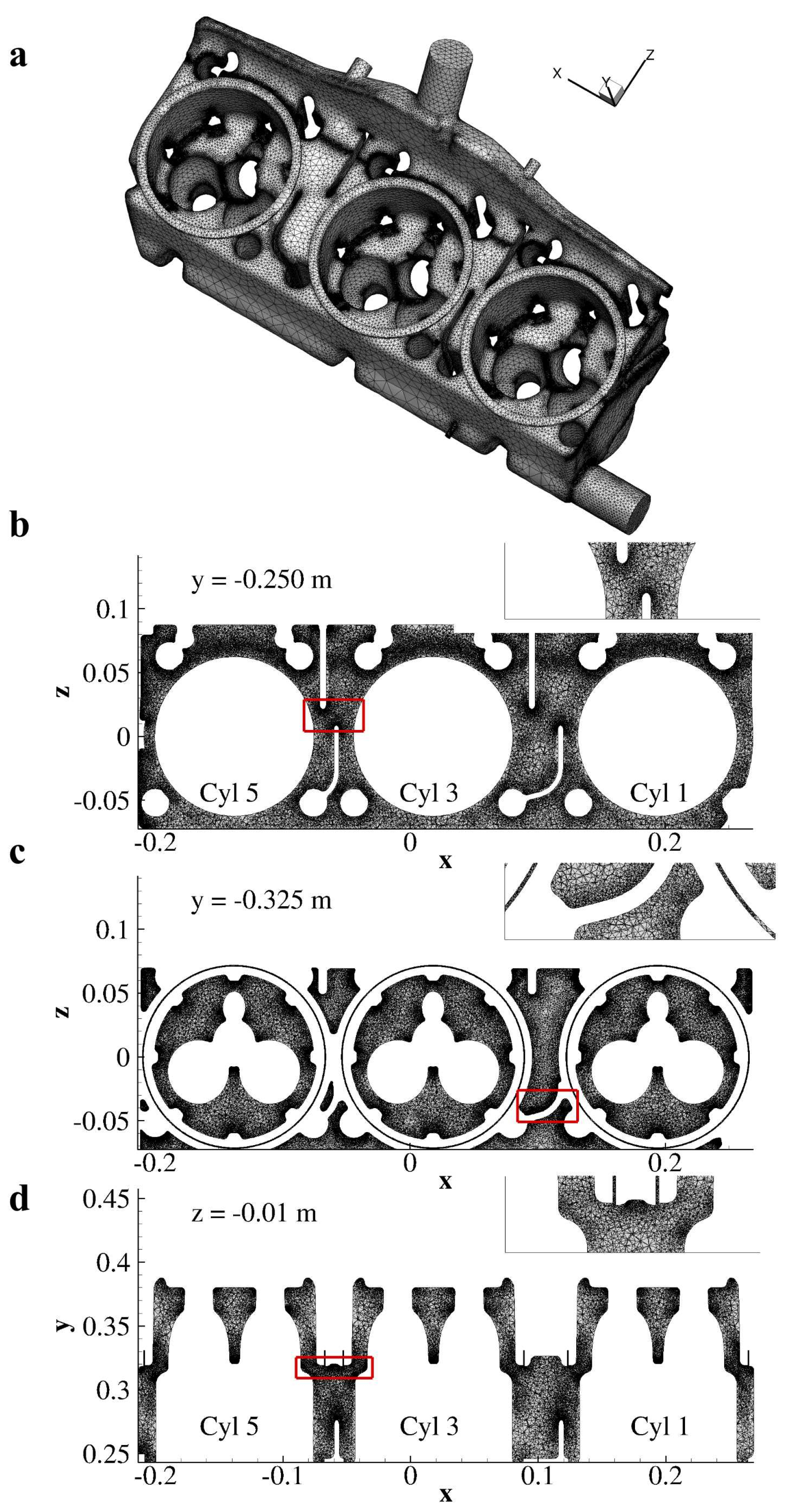
2.2. Computational Domain and Boundary Conditions

In this work, a six-cylinder aircraft compression ignition engine with two opposite banks is considered. Specifically, due to the specular geometries of the banks, only one of the two cooling system banks is considered (Figure 1a). The bank is characterized by an inlet section and an outlet section and presents three slots corresponding to the three cylinders jackets. Moreover, two modifications of this geometry are proposed and discussed to provide improvements in terms of mass-averaged outflow temperature and cylinder specific and total transferred thermal power (see Figure 1b,c). These geometries are discretized by means of about 8,000,000 tetrahedral elements with an average cell size of about 1.5 mm and a global minimum size of about 0.05 mm. The spatial discretization used in the computations for the single-inlet geometry (depicted in Figure 1a) is shown in Figure 2. Three sections are considered along with close-ups to show the quality of the discretization in the near-wall regions. Specifically, two transversal sections are located at y = −0.250 m and y = −0.325 m and the longitudinal section corresponds to the valve plane at z = −0.01 m. The minimum and maximum $y^{+}$ for this numerical discretization are 20 and 97, respectively. These values are well confined in the range of $10\le y^{+}\le 300$, which represents a constraint for the employed k–$ϵ$ closure joined with the use of standard wall functions.

The comparison between the three geometries is provided in terms of both the thermodynamic and kinematic flow fields, i.e., velocity, vorticity and temperature distributions, and of the evaluation of the pressure loss through the bank, the outflow temperature, as well as the cylinder specific and total transferred thermal power. To this end, two sets of simulations with five inlet mass-flow rates, namely $G_{in}=$ 0.5, 1.0, 1.5, 2.0, and 2.5 kg/s are considered. At first instance, thermal effects are neglected, i.e., fluid temperature is constant through the bank. This analysis is mainly carried out to provide a picture of the overall flow structure and to identify flow features under such an assumption. The working fluid is assumed to be water at 353 K with density and viscosity equal to 972 kg/s and 3.54 × 10${}^{-4}$ Pa·s, respectively. The second set of computations includes heat transfer between fluid and walls with the inlet coolant water temperature equal to 343 K and the crankcase external temperature equal to 380 K, whereas the cylinder jacket temperature ranges from 400 K to 460 K. For such thermal analysis, the water density and viscosity are computed as functions of the water temperature by employing a second-order polynomial fitting [24]. For both sets of computations, the mass-flow rate is set at the inlet section with an outlet pressure p${}_{out}=1$ bar. As regards turbulence, the inlet turbulence intensity is $u_{in}^{\prime }=0.25u_{in}$ and the turbulence characteristic length is equal to $0.3d_{in}$, being $d_{in}$ and $u_{in}$ the inlet diameter and the inlet mass-averaged fluid velocity, respectively.

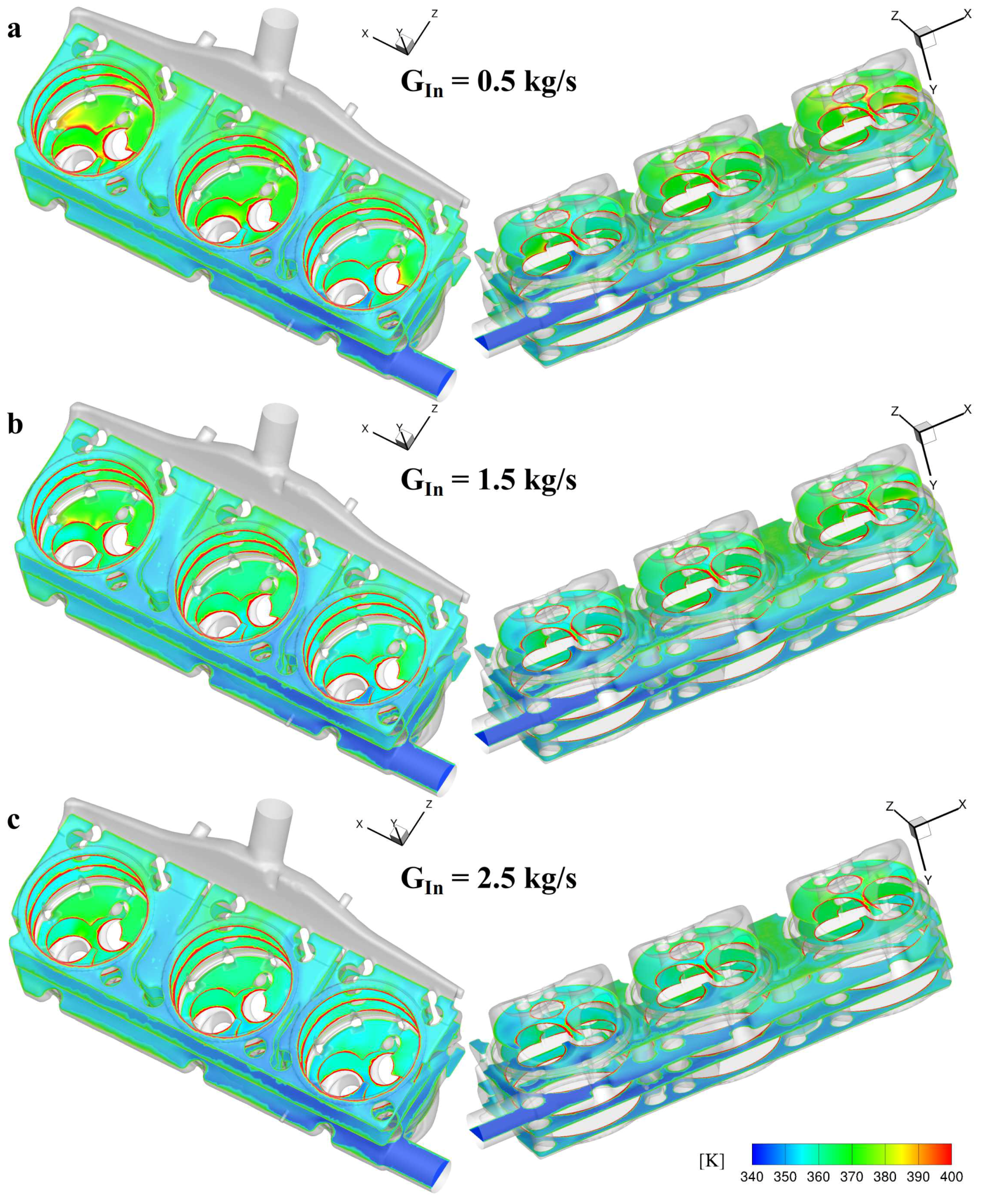
3. Results and Discussion

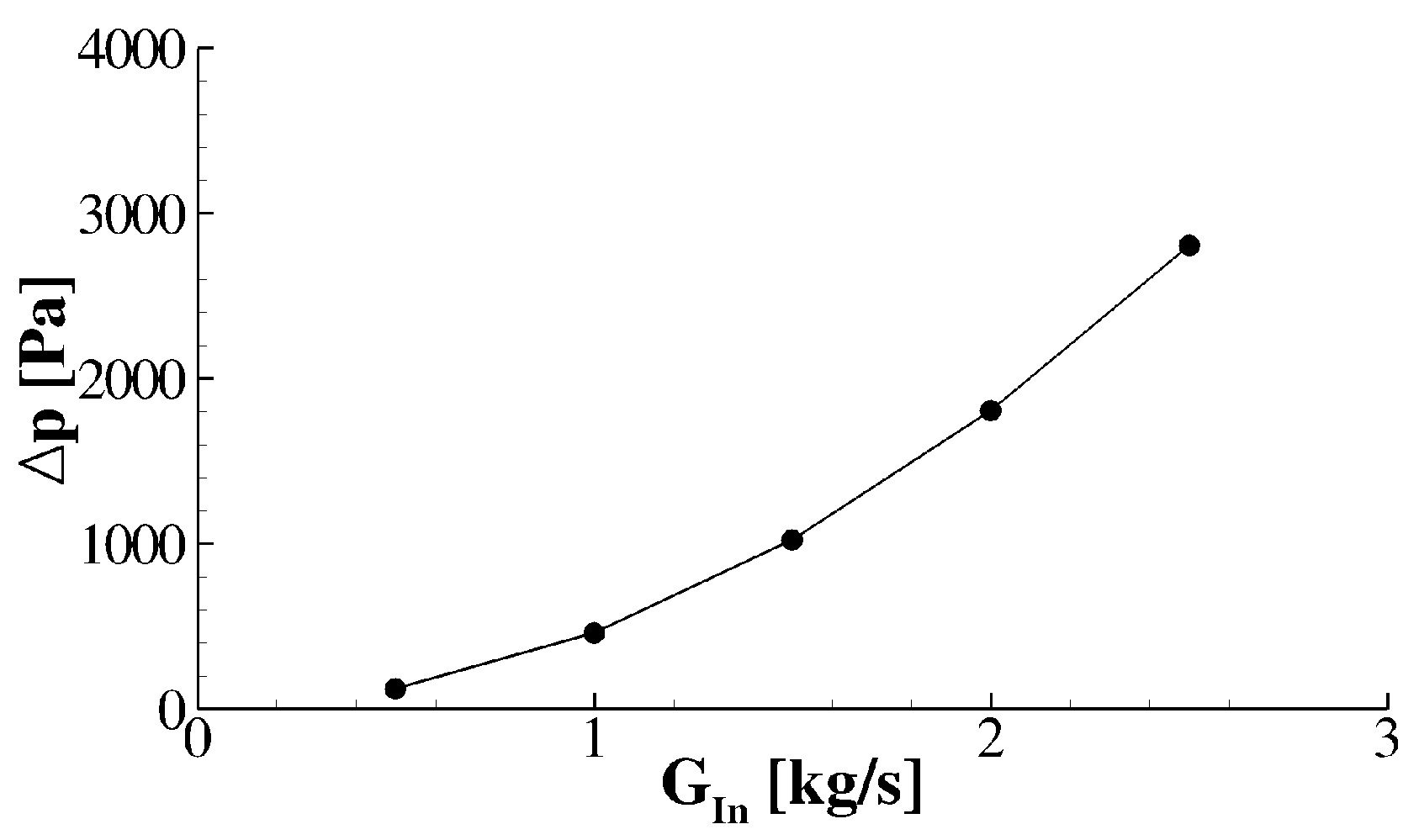
3.1. Analysis of the Single-Inlet Geometry

At first instance, the flow field of the single-inlet geometry (see Figure 1a) is analyzed by neglecting thermal effects. The pressure drop across the cooling system is computed as a function of the inlet mass-flow rate and shown in Figure 3. The head losses are computed as the difference between the inlet ($<p_{in}>$) and the outlet ($<p_{out}>$) surface-averaged pressure, $\mathsf{\Delta }p=<p_{in}{>}_{A_{in}}-<p_{out}{>}_{A_{out}}$, where $<p_{in/out}{>}_{A_{in/out}}$ correspond to the surface-averaged pressure related to the inlet (outlet) sections. The diagram shows that $\mathsf{\Delta }p$ vs. G${}_{in}$ follows a quadratic trend due to the fully developed turbulent regime of the flow field. The figure shows that $\mathsf{\Delta }p$ is of the order of 10${}^{-2}$ bar for all the investigated inlet mass-flow rates.

The velocity and vorticity magnitude contour plots, given in Figure 4, show that a large fraction of the flow pattern sweeps over the cylinder that is closer to the inlet section, i.e., cylinder 5. Then, the flow is almost totally short-circuited from the inlet directly to the outlet for all values of G${}_{in}$. Indeed, the cylinder in between, i.e., cylinder 3, is directly affected by the fluid flow, whereas cylinder 1 results poorly cooled down even for large values of G${}_{in}$, as shown in Figure 4c. On the other hand, the small values of $\mathsf{\Delta }p$ (O$\left({10}^{-2}\right)$ bar) reflect that the flow is somehow short-circuited so that the path actually performed by the fluid is relatively short and without much cross-sectional area variations. An interesting view of the flow structure is given in Figure 5 for G${}_{In}$ = 0.5, 1.5, and 2.5 kg/s, where the velocity magnitude colored streamlines are drawn to provide a qualitative picture of the coolant internal flow structure.

In order to consider thermal effects, the temperatures of the inlet water and of the crankcase are kept constant and equal to 343 K and 380 K, respectively. Several simulations have been performed by changing the cylinder jackets temperatures (T${}_{Cyls}$) from 400 to 460 K with a 20 K step. For the sake of conciseness, only the temperature contour plots for the case T${}_{Cyls}$ = 440 K are reported in Figure 6. Like the velocity and the vorticity patterns, the fluid temperature field clearly shows that the highest temperature is located around cylinder 1, regardless of G${}_{in}$. The water, flowing through cylinder 5 jacket, results colder than that through cylinder 3 jacket which is colder than that through cylinder 1 jacket. As regards the mass-averaged outflow temperature,

Table 1. Mass-averaged temperature, cylinder-specific and total transferred heat flux for T${}_{Cyls}$ = 440 K and G${}_{In}$ = 0.5, 1.0, 1.5, 2.0, and 2.5 kg/s obtained considering the single-inlet geometry.

G${}_{\mathit{In}}$ [kg/s]	T${}_{\mathit{Out}}$ [K]	Q${}_5$ [kW]	Q${}_3$ [kW]	Q${}_1$ [kW]	Q${}_{\mathit{Tot}}$ [kW]
0.5	362.6	9.6	6.9	4.4	40.8
1.0	360.2	17.5	11.4	6.7	71.4
1.5	359.2	25.4	16.3	9.0	100.7
2.0	358.7	32.9	21.3	11.4	130.3
2.5	358.5	40.8	25.9	13.9	160.5

shows that T${}_{Out}$ decreases, by increasing G${}_{In}$, with a smaller rate with respect to the mass flow rates (see Figure 7a). Besides, Table 1 shows the cylinder-specific and the total heat transferred. The cylinder-specific heat is computed by considering only the numerical cells that surround each cylinder, whereas the total heat is the sum over all the cells of the computational domain. The values of Table 1 clearly show that the cooling of the cylinder reduces as the distance between the cylinders and the inlet section increases. Specifically, the cylinder closest to the inlet transfers to the fluid a thermal power that is 2 to 3 times that of the furthest cylinder. ${\dot{Q}}_{Tot}$ increases linearly with G${}_{In}$ as depicted in Figure 7b. The distributions of T${}_{Out}$ for T${}_{Cyls}$ = 400, 420, 440, and 460 K are summarized in Figure 7c. Indeed, the functional form of these distributions is roughly constant with respect to the parameter T${}_{Cyls}$, while the distributions themselves are displaced with an offset which varies between 1.3 and 1.7 K. Two convenient thresholds for both the mass-averaged outflow temperature and the total transferred heat flux have been selected, which are superimposed to Figure 7c,d. T${}_{Out}$ has been supposed to be lower than 363 K since too high values would represent an inefficient cooling for the engine itself. Besides, since the output mechanical power of the six-cylinder engine ranges from 200 to 250 kW, the total transferred heat flux for each bank should range from 100 to 120 kW. The second condition is more stringent than the first and returns only some of the couples (T${}_{Cyl}$, G${}_{In}$) which are acceptable in the parameter space spanned with the simulations. The physically acceptable parameters are enlighten in

Table 2. Mass-averaged outflow temperature and total transferred heat flux tabulated as a function of G${}_{In}$ and T${}_{Cyls}$ for the single-inlet geometry.

	T${}_{\mathit{Cyls}}$ = 400 K		T${}_{\mathit{Cyls}}$ = 420 K		T${}_{\mathit{Cyls}}$ = 440 K		T${}_{\mathit{Cyls}}$ = 460 K
G${}_{\mathit{In}}$ [kg/s]	T${}_{\mathit{Out}}$ [K]	Q${}_{\mathit{Tot}}$ [kW]	T${}_{\mathit{Out}}$ [K]	Q${}_{\mathit{Tot}}$ [kW]	T${}_{\mathit{Out}}$ [K]	Q${}_{\mathit{Tot}}$ [kW]	T${}_{\mathit{Out}}$ [K]	Q${}_{\mathit{Tot}}$ [kW]
0.5	359.3	33.7	360.9	37.1	362.6	40.8	364.3	44.3
1.0	357.1	58.7	358.7	65.1	360.2	71.4	361.7	77.8
1.5	356.3	82.4	357.9	92.7	359.2	100.7	360.7	109.9
2.0	355.8	107.1	357.4	119.3	358.7	130.3	360.2	142.3
2.5	355.5	129.0	357.0	145.6	358.5	160.5	359.9	175.3

.

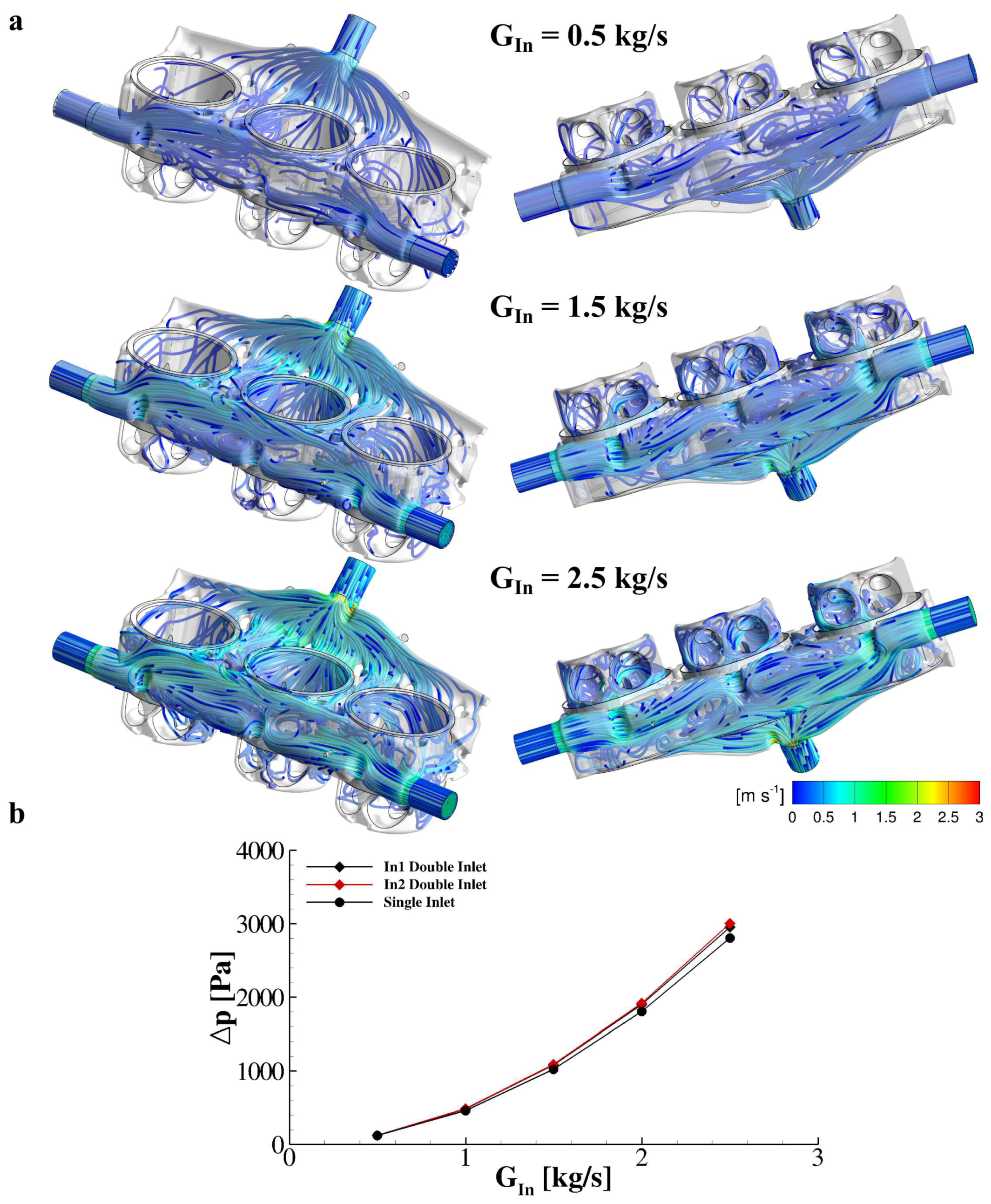
3.2. A First Cooling Improvement: The Double-Inlet Geometry

To overcome the uneven distribution of the cylinder-specific heat transfer with the single inlet geometry, a first simple geometrical modification is to double the intake manifold but with the same total inlet mass-flow rate G${}_{In}$, as reported in Figure 1b. Specifically, the second inlet section is placed close to cylinder 1 to promote heat transfer for this cylinder. The non-thermal analysis is firstly considered and shown in Figure 8. The internal flow streamlines depict an even distribution of the fluid between the three cylinders. Nonetheless, it must be stressed that the up-left region close to cylinder 1 results in the less-cooled region regardless of G${}_{In}$. This is qualitatively given in Figure 8a for G${}_{In}$ = 0.5, 1.5, and 2.5 kg/s. The head losses computed separately for both inlets as a function of G${}_{In}$ are comparable to the single inlet geometry case as shown in Figure 8c, where G${}_{In}$ is the total mass flow rate through the two inlets.

In order to account for the thermal effects, with the same fashion as per the single inlet geometry, the mass-averaged outflow temperature, as well as the cylinder-specific and the total transferred heat, are computed as a function of both G${}_{In}$ and T${}_{Cyls}$. These data are given in

Table 3. Mass-averaged temperature, cylinder-specific and total transferred heat flux for T${}_{Cyls}$ = 440 K and G${}_{In}$ = 0.5, 1.0, 1.5, 2.0, and 2.5 kg/s when considering the double-inlet geometry.

G${}_{\mathit{In}}$ [kg/s]	T${}_{\mathit{Out}}$ [K]	Q${}_5$ [kW]	Q${}_3$ [kW]	Q${}_1$ [kW]	Q${}_{\mathit{Tot}}$ [kW]
0.5	361.2	6.0	6.1	5.8	35.8
1.0	358.1	9.7	9.9	9.4	58.9
1.5	357.2	13.9	13.5	13.3	82.6
2.0	356.5	17.6	17.2	17.3	104.5
2.5	356.3	21.5	20.9	21.2	128.5

for T${}_{Cyls}$ = 440 K. Regardless of G${}_{In}$, the double inlet geometry returns outflow temperatures somewhat smaller than those of the single inlet geometry. Moreover, although an almost perfectly even distribution of transferred heat among the three cylinders, the total transferred thermal power is about 12-20% less than the previous geometry (see Table 1). This is because, even with a second inlet section, this geometry provides less cooling than the previous geometry. Indeed, it must be pointed out that the total intake mass-flow rate is the same as before but supplied by the two inlets. This reduces the amount of coolant fluid flowing into the system from each inlet, so that cylinder 5 jacket exchanges less heat with the less supplied water. As regards cylinder 3 and cylinder 1, the amount of water is about the same of cylinder 5 but not enough to efficiently cool down the overall system. For all of the investigated values of T${}_{Cyls}$, the total transferred heat and the outflow temperatures are given in

Table 4. Mass-averaged outflow temperature and total transferred heat flux tabulated as a function of G${}_{In}$ and T${}_{Cyls}$ for the double inlet geometry.

	T${}_{\mathit{Cyls}}$ = 400 K		T${}_{\mathit{Cyls}}$ = 420 K		T${}_{\mathit{Cyls}}$ = 440 K		T${}_{\mathit{Cyls}}$ = 460 K
G${}_{\mathit{In}}$ [kg/s]	T${}_{\mathit{Out}}$ [K]	Q${}_{\mathit{Tot}}$ [kW]	T${}_{\mathit{Out}}$ [K]	Q${}_{\mathit{Tot}}$ [kW]	T${}_{\mathit{Out}}$ [K]	Q${}_{\mathit{Tot}}$ [kW]	T${}_{\mathit{Out}}$ [K]	Q${}_{\mathit{Tot}}$ [kW]
0.5	357.6	27.7	359.7	32.6	361.6	35.8	362.7	38.9
1.0	355.6	48.3	356.9	53.6	358.1	58.9	359.5	65.0
1.5	354.8	67.6	356.0	75.1	357.2	82.6	358.4	90.3
2.0	354.3	86.2	355.5	96.0	356.5	104.5	357.8	115.7
2.5	353.9	104.5	355.1	116.5	356.3	128.5	357.4	140.5

which reflects the same picture drawn for the single inlet geometry.

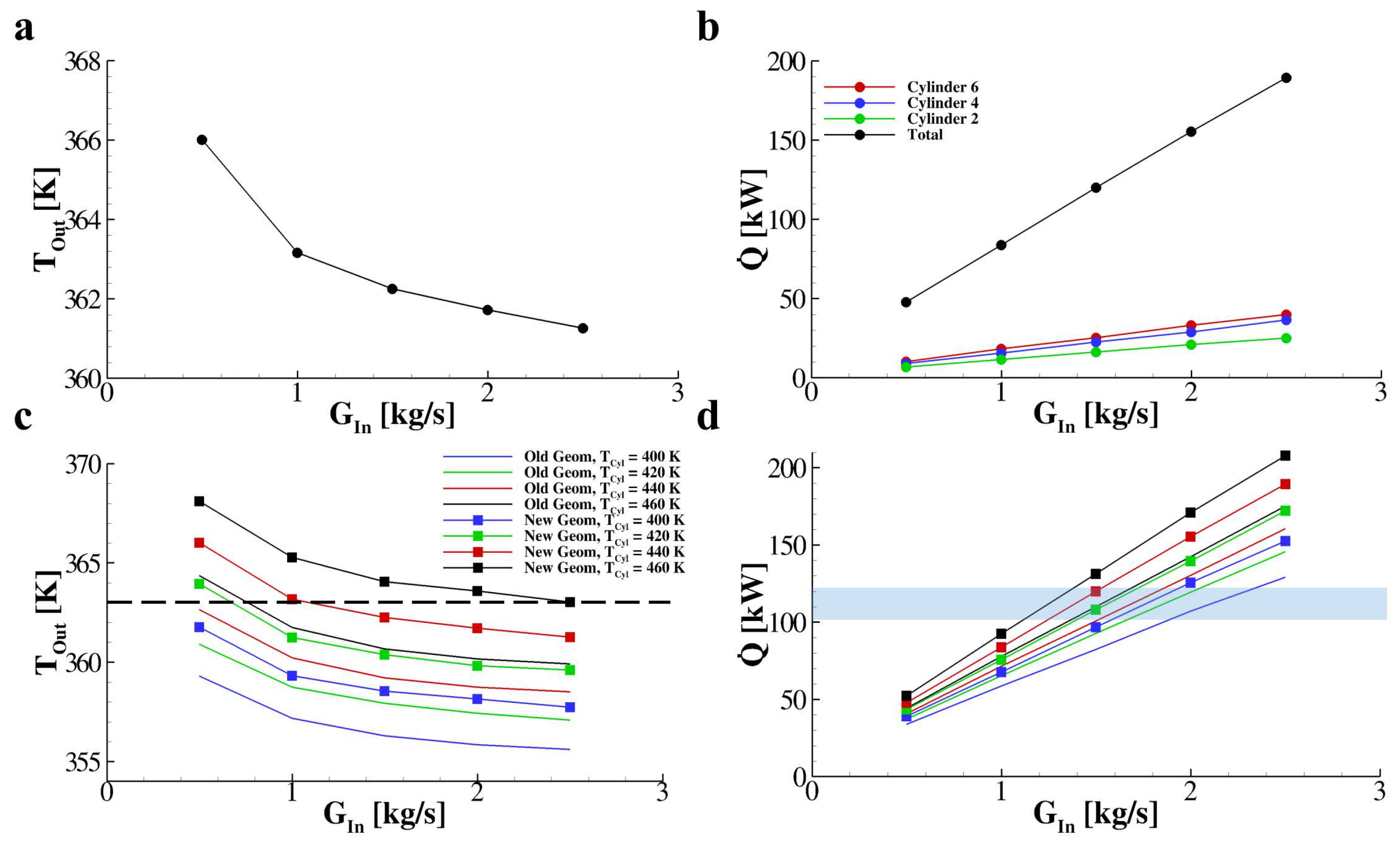
3.3. A New Single Inlet Geometry

An interesting geometrical improvement for the cooling system is proposed in Figure 1c. This new geometry is shown for the left bank of the cooling system. Indeed, right and left banks slightly differ due to the quasi-symmetric position of the cylinder seats. However, these differences are negligible for the purposes of the present work. Specifically, the geometrical improvement is twofold. On one hand, the geometry considers some enlargements and restrictions within the bank (see the intra-cylinder jackets regions), and, on the other hand, the outlet manifold is moved from the inlet section. In this context, enlargements and restrictions are designed to guide the flow from the inlet through all of the three-cylinder jackets and then to the outflow section, while the outlet is placed between cylinder 4 and cylinder 2 to avoid any possible short-circuiting of the flow itself. The velocity magnitude colored streamlines of the simulations without thermal effects for the new geometry are depicted in Figure 9a for G${}_{In}$ = 0.5, 1.5 and 2.5 kg/s. The figure shows that the fluid flow supplies, almost uniformly, the three-cylinder jackets and reaches the outlet section without being short-circuited. Indeed, the water flowing over the three cylinders results enhanced for large values of the intake mass-flow rate as shown by the increased number of streamlines sweeping over the jackets and the cylinder heads. Moreover, the increasing complexity of the flow path with respect to the previous single-inlet geometry, due to the provided enlargements and restrictions, reflects into an increase of $\mathsf{\Delta }p$, as shown in Figure 9b.

Thermal effects are also considered in order to analyze the cooling efficiency of this new geometry in terms of computed temperature field, mass-averaged outflow temperature and total transferred heat. As shown in Figure 10, the temperature field results quite homogeneous with respect to the old single-inlet geometry. Specifically, for G${}_{In}$ = 0.5 kg/s, around the farthest cylinder jacket from the inlet, i.e., cylinder 1, a temperature between 370 and 380 K is computed for the old geometry (see Figure 6a) whereas, for the new geometry the farthest cylinder jacket from the inlet, i.e., cylinder 2, provides a temperature between 360 and 370 K. This improvement is also quantitatively assessed by the outflow mass-average temperature in

Table 5. Mass-averaged temperature, cylinder-specific and total transferred heat flux for T${}_{Cyls}$ = 440 K and G${}_{In}$ = 0.5, 1.0, 1.5, 2.0, and 2.5 kg/s when considering the new geometry.

G${}_{\mathit{In}}$ [kg/s]	T${}_{\mathit{Out}}$ [K]	Q${}_6$ [kW]	Q${}_4$ [kW]	Q${}_2$ [kW]	Q${}_{\mathit{Tot}}$ [kW]
0.5	366.0	10.1	9.0	6.8	47.9
1.0	363.1	18.3	15.5	11.4	83.7
1.5	362.2	25.1	22.5	16.3	119.9
2.0	361.5	33.2	28.9	20.8	155.3
2.5	361.2	39.9	36.4	25.0	189.4

. Indeed, for the T${}_{Cyls}$ = 440 K case, T${}_{Out}$ is higher for the new geometry with respect to the old configuration. Moreover, an improvement of about 20% for the total transferred thermal power is observed for all the investigated G${}_{In}$. All of those data are summarized in Figure 11a,b for T${}_{Out}$ and $\dot{Q}$, respectively. A direct comparison between the two single inlet geometries is obtained by considering T${}_{Out}$ and $\dot{Q}$ as a function of G${}_{In}$ and T${}_{Cyls}$ and depicted in Figure 11c,d. Regardless of the cylinder jacket wall temperatures, the outflow water temperature was higher with the new configurations due to the larger amount of thermal power (≈20%) transferred to the water. As per the old geometry, two thresholds are considered. The outflow temperature threshold is set to 363 K while the bandwidth for $\dot{Q}$ corresponds to 110 kW ± 10 kW. The practical values in the spanned parameter space are enlightened in

Table 6. Mass-averaged outflow temperature and total transferred heat flux tabulated as a function of G${}_{In}$ and T${}_{Cyls}$ for the new geometry.

	T${}_{\mathit{Cyls}}$ = 400 K		T${}_{\mathit{Cyls}}$ = 420 K		T${}_{\mathit{Cyls}}$ = 440 K		T${}_{\mathit{Cyls}}$ = 460 K
G${}_{\mathit{In}}$ [kg/s]	T${}_{\mathit{Out}}$ [K]	Q${}_{\mathit{Tot}}$ [kW]	T${}_{\mathit{Out}}$ [K]	Q${}_{\mathit{Tot}}$ [kW]	T${}_{\mathit{Out}}$ [K]	Q${}_{\mathit{Tot}}$ [kW]	T${}_{\mathit{Out}}$ [K]	Q${}_{\mathit{Tot}}$ [kW]
0.5	361.7	38.9	363.9	43.5	366.0	47.9	368.1	52.1
1.0	359.3	67.7	361.2	75.7	363.1	83.7	365.2	92.5
1.5	358.5	96.6	360.3	108.1	362.2	119.9	364.0	131.1
2.0	358.1	125.5	359.8	139.4	361.5	155.3	363.5	170.9
2.5	357.7	152.4	359.6	172.0	361.2	189.4	363.0	207.9

.

4. Conclusions

In this work multi-dimensional CFD is employed to enhance the performance of the cooling system of an aircraft engine. Capabilities and limitations of different geometries are highlighted, in order to give guidelines as regards an efficient design of the engine. The analysis is carried out by means of a finite-volume RANS equations solver with k-$ϵ$ closure.

An initial configuration of the cooling system without any thermal effects is firstly considered, with constant temperature, density and viscosity for the water. The pressure loss of the cooling system as a function of the inlet mass-flow rate is computed. Velocity and vorticity patterns are also given to point out features of the flow field. Then, thermal effects are taken into account and the cooling performance of such a configuration is assessed as a function of both the inlet mass-flow rate and the cylinder jackets temperatures. Specifically, the outflow temperature and both the total and the cylinder-specific transferred thermal power are computed. This geometry is demonstrated to be not very efficient because the cylinder-specific transferred heat decreases as the distance between the cylinders and the intake section increases.

Two geometrical improvements are then proposed: first, the inlet sections are doubled while keeping the same total mass-flow rate; second, a new single-inlet geometry is designed by inserting restrictions and enlargements within the cooling system to constrain the coolant flow and by moving downstream the outflow duct. The double-inlet geometry exchanges less thermal power than the initial single inlet geometry (≈12-20%) with an almost perfectly even cylinder-specific transferred heat distribution. The new single inlet geometry improves the overall abilities of the cooling system of about 20% (referring to the total transferred thermal power) while keeping the three cylinders only slightly unevenly cooled. Moreover, the new single-inlet geometry presents, as expected, an increase of the characteristic loads due to the restrictions and enlargements within the flow field. However, since this head loss represents only about 10% of the total head loss of the whole cooling circuit, the new single-inlet geometry may be a reasonable choice to optimize the efficiency of the cooling system.

References

1. Jacobs, T.J. Internal Combustion Engines, Developments in. In Fossil Energy; Malhotra, R., Ed.; Encyclopedia of Sustainability Science and Technology Series; Springer: New York, NY, USA, 2020; pp. 133–184. ISBN 978-1-4939-9762-6. [Google Scholar] [CrossRef]
2. Ryuichi, M.; Toshihiko, I.; Hiroyuki, F.; Yasutoshi, Y. Internal combustion engine cooling apparatus. App. Therm. Eng. 1996, 16, 101–132. [Google Scholar] [CrossRef]
3. Griffiths, J.; Barnard, J. Flame and Combustion; Routledge: Abingdon, UK, 2019; ISBN 9780203755976. [Google Scholar] [CrossRef]
4. Zhukov, V.; Melnik, O.; Logunov, N.; Chernyi, S. Regulation and control in cooling systems of internal combustion engines. E3S Web Conf. 2019, 02015, 135. [Google Scholar] [CrossRef]
5. Farokhi, S. Future Propulsion Systems and Energy Sources in Sustainable Aviation; John Wiley & Sons: Hoboken, NJ, USA, 2020. [Google Scholar] [CrossRef]
6. Vasilyev, A.V.; Lartsev, A.; Fedyanov, E. Evaluation of Possible Limits of Forcing of High-Capacity Air-Cooled Engines. In Proceedings of the International Conference on Industrial Engineering, Sochi, Russia, 25–29 March 2019; Springer: Berlin, Germany, 2019. [Google Scholar] [CrossRef]
7. Bleier, F.; Bauer, H. Prediction of Heat Transfer in a Jet Cooled Aircraft Engine Compressor Cone Based on Statistical Methods. Aerospace 2018, 5, 51. [Google Scholar] [CrossRef] [Green Version]
8. Jafari, S.; Nikolaidis, T. Thermal Management Systems for Civil Aircraft Engines: Review, Challenges and Exploring the Future. Appl. Sci. 2018, 8, 2044. [Google Scholar] [CrossRef] [Green Version]
9. Wang, D.; Naterer, G.; Wang, G. Adaptive response surface method for thermal optimization: Application to aircraft engine cooling system. In Proceedings of the 8th AIAA/ASME Joint Thermophysics and Heat Transfer Conference, St. Louis, MO, USA, 24–26 June 2002. [Google Scholar] [CrossRef]
10. Jaffe, R.; Taylor, W. The Physics of Energy; Cambridge University Press: Cambridge, UK, 2018. [Google Scholar]
11. Jaffe, R.; Taylor, W. Internal Combustion Engines; Cambridge University Press: Cambridge, UK, 2019; pp. 203–218. [Google Scholar] [CrossRef]
12. Aschemann, H.; Prabel, R.; Gross, C.; Schindele, D. Flatness-based control for an internal combustion engine cooling system. In Proceedings of the 2011 IEEE International Conference on Mechatronics, Istanbul, Turkey, 13–15 April 2011; pp. 140–145. [Google Scholar] [CrossRef]
13. Petrov, A.P.; Bannikov, S.N. Active Shutters of the Internal Combustion Engine Cooling System of a Passenger Car. In Proceedings of the Higher Educational Institutions, Palma, Spain, 1–3 July 2019; pp. 44–51. [Google Scholar] [CrossRef]
14. Razuvaev, A.; Slobodina, E. The operating conditions of the internal combustion engine with high temperature cooling. J. Phys. Conf. Ser. 2020, 1441, 120–126. [Google Scholar] [CrossRef]
15. Keskinen, K.; Nuutinen, M.; Kaario, O.; Vuorinen, V.; Jann, K.; Wright, Y.M.; Larmi, M.; Boulouchos, K. Hybrid LES/RANS with wall treatment in tangential and impinging flow configurations. Int. J. Heat Fluid Flow 2017, 65, 141–158. [Google Scholar] [CrossRef]
16. Krastev, V.K.; Silvestri, L.; Bella, G. Effects of turbulence modeling and grid quality on the zonal URANS/LES simulation of static and reciprocating engine-like geometries. SAE Int. J. Eng. 2018, 11, 669–686. [Google Scholar] [CrossRef]
17. Krastev, V.K.; Di Ilio, G.; Falcucci, G.; Bella, G. Notes on the hybrid URANS/LES turbulence modeling for Internal Combustion Engines simulation. Energy Procedia 2018, 148, 1098–1104. [Google Scholar] [CrossRef]
18. Chorin, A.J. Numerical solution of the Navier-Stokes equations. Math. Comput. 1968, 22, 745–762. [Google Scholar] [CrossRef]
19. Patankar, S.V.; Spalding, D.B. A calculation procedure for heat, mass and momentum transfer in three-dimensional parabolic flows. Int. J. Heat Mass Transfer 1972, 15, 54–73. [Google Scholar] [CrossRef]
20. Anderson, W.K.; Bonhaus, D.L. An implicit upwind algorithm for computing turbulent flows on unstructured grids. Comput. Fluids 1994, 23, 1–21. [Google Scholar] [CrossRef] [Green Version]
21. Barth, T.; Jespersen, D. The design and application of upwind schemes on unstructured meshes. In Proceedings of the 27th Aerospace Sciences Meeting, Reno, NV, USA, 9–12 January 1989; pp. 366–390. [Google Scholar]
22. Hutchinson, B.R.; Raithby, G.D. A multigrid method based on the additive correction strategy. Numer. Heat Transf. Part A Appl. 1986, 9, 511–537. [Google Scholar]
23. Launder, B.E.; Spalding, D.B. The numerical computation of turbulent flows. Comput. Methods Appl. Mech. Eng. 1974, 3, 269–289. [Google Scholar] [CrossRef]
24. Likhachev, E.R. Dependence of Water Viscosity on Temperature and Pressure. Tech. Phys. 2003, 48, 4. [Google Scholar] [CrossRef]
Figure 1. Geometry of the cooling system for the three configurations. (a) Sketch of the right bank of the cooling system. (b) Sketch of the right bank of the cooling system with a second intake duct (In2) on the opposite side with respect to the old one (In1). (c) Sketch of a new single inlet geometry (left bank) obtained by inserting enlargements and restrictions to the old one and by moving downstream the outlet duct. All of the graphics are represented from an internal (left column) and external (right column) point of view.
Fluids 05 00071 g001
Figure 2. Spatial discretization of the cooling system for the single-inlet configuration. (a) Computational mesh of the right bank of the cooling system. (b,c) Transversal sections of the computational mesh at (b) y = −0.250 m and (c) y = −0.325 m. (d) Longitudinal section of the computational mesh at the valve plane z = −0.01 m.
Fluids 05 00071 g002
Figure 3. Single-inlet cooling system characteristic loads. Pressure loss as a function of the inlet mass-flow rate.
Fluids 05 00071 g003
Figure 4. Velocity and vorticity contour plots for the single-inlet geometry. Distribution of velocity (left) and vorticity (right) magnitude for G I n = 0.5 (a), 1.5 (b), and 2.5 (c) kg/s.
Fluids 05 00071 g004
Figure 5. Velocity magnitude colored streamlines for the single-inlet geometry. Velocity magnitude colored streamlines, starting from the inlet section, for G I n = 0.5 (a), 1.5 (b), and 2.5 (c) kg/s. Internal (left) and external (right) point of view.
Fluids 05 00071 g005
Figure 6. Temperature patterns for T C y l s = 440 K for the single-inlet geometry. Temperature contour plots for T C y l s = 440 K and G I n = 0.5 (a), 1.5 (b), and 2.5 (c) kg/s.
Fluids 05 00071 g006
Figure 7. Outflow temperature and transferred heat flux for the single-inlet geometry. (a) Mass-averaged outflow temperature as a function of G I n for T C y l s = 440 K. (b) Cylinder specific and total transferred heat flux as a function of G I n for T C y l s = 440 K. (c) Mass-averaged outflow temperature as a function of G I n for T C y l s = 400, 420, 440, and 460 K. (d) Total transferred heat flux as a function of G I n for T C y l s = 400, 420, 440, and 460 K.
Fluids 05 00071 g007
Figure 8. Velocity streamlines and characteristic loads for the double-inlet geometry. (a) Velocity magnitude colored streamlines obtained for the double-inlet geometry for G I n = 0.5, 1.5 and 2.5 kg/s. (b) Distribution of the pressure loss as a function of the inlet mass-flow rate.
Fluids 05 00071 g008
Figure 9. Velocity streamlines and characteristic loads for the new single-inlet geometry. (a) Velocity magnitude colored streamlines obtained for the new single-inlet geometry for G I n = 0.5, 1.5 and 2.5 kg/s (b) Pressure loss as a function of the inlet mass-flow rate.
Fluids 05 00071 g009
Figure 10. Temperature patterns for the new single-inlet geometry. Temperature contour plots obtained for T C y l s = 440 K and G I n = 0.5 (a), 1.5 (b), and 2.5 (c) kg/s.
Fluids 05 00071 g010
Figure 11. Outflow temperature and transferred heat flux for the new geometry. (a) Mass-averaged outflow temperature as a function of G I n for T C y l s = 440 K. (b) Cylinder specific and total transferred heat flux as a function of inlet mass-flow rate for T C y l s = 440 K. (c) Comparison of the mass-averaged outflow temperature as a function of G I n and T C y l s between the old and the new single-inlet geometry. (d) Total transferred heat flux as a function of the inlet mass-flow rate obtained with the old and the new geometry.
Fluids 05 00071 g011