
Ocean Convection


1
Department of Mechanical Engineering, University of Melbourne, Melbourne, VIC 3010, Australia
2
Centre for Atmospheric and Oceanic Sciences, Indian Institute of Science, Bangalore 560012, India
*
Authors to whom correspondence should be addressed.
Fluids 2021, 6(10), 360; https://doi.org/10.3390/fluids6100360
Submission received: 18 June 2021
/
Revised: 24 September 2021
/
Accepted: 24 September 2021
/
Published: 12 October 2021
(This article belongs to the Special Issue Ocean Convection)
Abstract
:Ocean convection is a key mechanism that regulates heat uptake, water-mass transformation, CO2 exchange, and nutrient transport with crucial implications for ocean dynamics and climate change. Both cooling to the atmosphere and salinification, from evaporation or sea-ice formation, cause surface waters to become dense and down-well as turbulent convective plumes. The upper mixed layer in the ocean is significantly deepened and sustained by convection. In the tropics and subtropics, night-time cooling is a main driver of mixed layer convection, while in the mid- and high-latitude regions, winter cooling is key to mixed layer convection. Additionally, at higher latitudes, and particularly in the sub-polar North Atlantic Ocean, the extensive surface heat loss during winter drives open-ocean convection that can reach thousands of meters in depth. On the Antarctic continental shelf, polynya convection regulates the formation of dense bottom slope currents. These strong convection events help to drive the immense water-mass transport of the globally-spanning meridional overturning circulation (MOC). However, convection is often highly localised in time and space, making it extremely difficult to accurately measure in field observations. Ocean models such as global circulation models (GCMs) are unable to resolve convection and turbulence and, instead, rely on simple convective parameterizations that result in a poor representation of convective processes and their impact on ocean circulation, air–sea exchange, and ocean biology. In the past few decades there has been markedly more observations, advancements in high-resolution numerical simulations, continued innovation in laboratory experiments and improvement of theory for ocean convection. The impacts of anthropogenic climate change on ocean convection are beginning to be observed, but key questions remain regarding future climate scenarios. Here, we review the current knowledge and future direction of ocean convection arising from sea–surface interactions, with a focus on mixed layer, open-ocean, and polynya convection.
1. Introduction
Vertical buoyancy differences (specifically denser fluid on top of lighter fluid) drive convective plumes, which are associated with large vertical motions that transport heat, salinity, and tracers [1,2]. Atmospheric forcing at the air–sea interface can drive vigorous convection in the global ocean. Heat-loss at the ocean surface and surface water salinification (due to evaporation or sea-ice formation) are both mechanisms that densify the top of the water column. The resulting unstable water column can produce convective plumes that move downwards through the ocean depths. Depending on factors such as the strength of the buoyancy forcing and the ocean stratification, the convective plumes can be constrained to the mixed layer or penetrate to abyssal depths [3]. This review is focused on ocean convection forced by sea-surface interaction, including mixed layer convection, open-ocean convection, and polynya convection.
The upper-ocean mixed layer is a ubiquitous feature across almost the entire global ocean. The mixed layer is critical in modulating the ocean surface fluxes of heat, freshwater (precipitation and evaporation), and CO2. Convection is an important process maintaining the mixed layer, along with other physical mechanisms, such as wind stress, Langmuir turbulence, internal and surface waves, and more [4,5,6]. As part of the diurnal cycle, there is night-time cooling of the ocean surface. This rapid loss in buoyancy triggers convection, which mixes the top of the water column and helps to deepen the upper-ocean mixed layer. Mixed layer convection can also be triggered by evaporation that leads to densification of surface waters. The base of the mixed layer is capped by the strongly stratified pycnocline, limiting the layer depth to 10–100 m in summer and up to 500 m deep in some regions in winter (Figure 1). The mixed layer depth is also variable in space with a deeper mixed layer at higher latitudes during winter and in equatorial regions during summer, and the Southern Ocean having a deep mixed layer year-round [7].
In some regions of the ocean, particularly in winter, the surface buoyancy loss is strong enough to produce open-ocean convection that can penetrate through the surface layers into the abyssal ocean. Open-ocean convection mainly occurs in the North Atlantic Ocean, particularly in sub-polar regions where there can be intense, highly localized cooling of surface waters by the atmosphere in winter months. It can be noted that these locations, such as the Greenland Sea and Labrador Sea, have a generally higher sea-surface density than the rest of the global ocean (excepting the Southern Ocean) as shown in Figure 1b. Open-ocean convection can reach thousands of meters depth and is key ingredient for water-mass transformation [3], including the production of North Atlantic deep water (NADW) that feeds into the upper cell of the meridional overturning circulation (MOC).
The Southern Ocean is another key location for sea-surface water-mass transformation that further leads to convection. During winter, much of the ocean around Antarctica is covered in sea-ice, which inhibits atmosphere-ocean interactions. However, in some regions there are gaps in the sea-ice, known as polynyas, where upper-ocean waters experience huge buoyancy losses, and convection takes place. Coastal polynyas are common around the Antarctic continent, where katabatic winds push any newly formed sea-ice offshore. The wintertime sea-ice formation in these coastal polynyas can result in large amounts of brine rejection and significant densification of surface waters, triggering strong ocean convection. More sporadically, offshore polynyas have been observed far away from the coast of Antarctica in the Weddell Sea. In the winters of 1974–1976, a huge Weddell Sea polynya and vigorous convection was observed [10]. Since then, smaller polynya convection has been observed in some years near the Maud Rise oceanic plateau, but there remain questions on the triggers of offshore polynya convection [11,12]. Both coastal and offshore polynya convection are able to provide significant water-mass transformation and produce Antarctic bottom water (AABW), one of the densest water masses in the ocean, which feeds into the lower overturning cell of the MOC [12,13,14].
It is timely to review the observational data, laboratory experiments and numerical simulations on ocean convection. An early review of ocean convection was first conducted by Killworth [15] in 1983 and discussed both open-ocean and polynya convection. There was also an in-depth review on open-ocean convection by Marshall and Schott [3] in 1999 and a review of polynyas, including polynya convection, by Morales Maqueda et al. [16] in 2004. Since these reviews, there has been substantial progress made in terms of observing, modeling and understanding ocean convection. It is also worth noting that there are other highly important convective processes in the ocean, such as double-diffusive convection (due to the large difference in diffusivities between temperature and salinity) [17], convection arising from symmetric instability [18,19], convection beneath ice [20,21,22,23], subglacial plumes [24,25], convection driven by internal waves [26,27], and so on. These are each worthy of their own review but, due to length constraints, will not be covered here. This review will cover mixed layer convection, open-ocean convection and polynya convection in the remaining sections, followed by a summary and future direction.
2. Mixed Layer Convection
The mixed layer is the uppermost part of the marine surface waters that is characterized by its near-homogeneous density (temperature/salinity) distribution. Its dynamics directly impact critical parameters at the air–sea interfaces, such as the sea-surface temperature and salinity, and the near-surface air temperature and pressure. The mixed layer regulates the air–sea interactions (heat, precipitation/evaporation, and CO2), ocean biology and nutrient budget across the global ocean. Throughout the world’s oceans, the mixed layer depth (MLD) is maintained by various processes such as buoyancy-driven convection, Langmuir turbulence, surface wave breaking, sub-mesoscale frontal instability, shear or wind-driven mixing, and internal wave breaking [1,5,6,28]. Many of these processes are driven by atmospheric forcing related to the wind field and buoyancy fluxes. There has been some quantitative comparison of Langmuir turbulence, shear and convection effects using observations, which finds that different processes dominate the upper mixed layer for different times and locations, with some regions being strongly affected by all three processes at once [6,29]. At the base of the mixed layer there is a strong gradient of density (temperature/salinity) known as the pycnocline (thermocline/halocline) that caps the mixed layer turbulence from the relatively calm deep water below. The daily to seasonal cycle of heating and cooling, wind, rain, evaporation, and river run-off are a hierarchy of physical processes that constantly shape the upper-ocean mixed layer and are the primary causes of variation in the MLD. The observational data shows that the MLD is rapidly responding to various changing (mechanical and buoyancy) forcings from the changing climate [30]. In this section we discuss the various components of the buoyancy forcing, the upper-ocean response to the forcing, and the dynamics of the resulting convection. We also outline the diurnal and seasonal variability of the surface forcing and the impact on the MLD.
The net heat flux on the ocean surface is primarily made up of four components: shortwave (solar insolation; ), longwave (thermal infrared; ), sensible heat flux (heat transport due to conduction; ), and latent heat flux (evaporative cooling; ). The heat flux due to any precipitation () is typically very small [31]. The net heat flux at the air–ocean interface can then be written as,
where incoming shortwave and longwave radiative fluxes are shown by “↓” and outgoing by “↑”, respectively. Note that, where is the albedo of the ocean surface. When is positive, the ocean is heated by the atmosphere, while negative corresponds to cooling the ocean surface. In a similar manner to the sea-surface heat budget, the upper layer salinity is controlled by the sea-surface freshwater budget. The net salinity flux at the ocean surface is
where is the precipitation (rain or snow) rate (m s−1), is the evaporation rate, and is the sea-surface salinity. The rate of evaporation is further linked with the latent heat flux by , where is the water density and is the latent heat of evaporation.
When it comes to the diurnal timescale, the net heat flux follows the cycle of heating the ocean upper layer during the day-time and cooling during the night-time. This variability is attributed to the net shortwave component, which peaks at up to a surface irradiance of 800–1000 W/m2 during the day-time depending on the latitude, season and other factors, and vanishes at night-time (positive sign corresponds to heating of the ocean surface) [31]. Cloud cover during the day-time can significantly reduce the magnitude of the shortwave component. The other components predominantly provide a net cooling to the surface at all times, with major cooling contributions from latent heat flux and longwave radiation. The latent heat flux is due to evaporative cooling, which is relatively high around the tropics and subtropics ranging from −50 W/m2 to −150 W/m2 (negative sign indicates cooling). The evaporation rate also depends on the sea-surface wind stress, so when there is strong wind activity (e.g., a tropical cyclone) the evaporative cooling flux can reach as large as −500 W/m2. The value of the outgoing longwave radiation primarily depends on sea-surface temperature and ranges between −50 W/m2 to −60 W/m2. The sensible heat flux is, on average, negative across most of the globe, excepting a few specific locations at higher latitudes (around the Southern Ocean), for more detail about spatial variance see [31]. Over most of the global ocean, the sensible heat flux makes up the smallest fraction of net cooling heat flux and is an order of magnitude smaller that the longwave radiation. However, the sensible heat flux in the regions of the Gulf Stream and the Kuroshio (and also near Greenland) can reach large values in winter when relatively cold air from the continent blows over the warm western boundary current [32]. The diurnal cycle (of net heating during the day and net cooling during the night) is a distinct feature in weather systems over the tropics and sub-tropics, spanning roughly 40° N–40° S. Seasonality, with the appearance of summer and winter, becomes a common feature in the subtropical region, with the sub-polar and polar regions experiencing much more pronounced and prolonged winters and summers.
The upper-ocean responds very differently to the various types of ocean surface forcing. During the day-time, shortwave radiation penetrates the upper-ocean where the longer wavelengths (red and yellow) are absorbed in the top 5 m and the shorter wavelengths (blue and green) are absorbed at around 20 m depth [33]. The layer over which solar radiation penetrates is widely known as the diurnal warm layer [1,34,35]. The radiation attenuates approximately exponentially, with the rate of decay dependent on the turbidity of water [33]. This heats the upper-ocean and builds the stratification that further suppresses upper layer turbulent activity, resulting in a shallowing of the MLD [1,36]. The MLD during this period depends on the net surface heat flux and the amount of turbulent mixing [37] in the sub-surface through various mechanisms (primarily shear instability, baroclinic or symmetric instabilities, breaking of surface and near inertial waves, and Langmuir turbulence) [1,18]. In contrast, the non-solar fluxes (longwave radiation, evaporation, and sensible heat flux) typically provide continual cooling at the ocean surface.
Mixed layer convection can be triggered during the night-time, when the shortwave radiation shuts off and the ocean surface undergoes cooling. This results in water parcels at the surface having a higher density relative to water parcels at depth. The dynamics of the resulting convection includes the formation of cold convective plumes (Figure 2). These convective plumes have to overcome the viscous and diffusive forces, which are relatively high inside the very thin layer (known as the “ocean cool skin” [38]) immediately below the air-ocean interface. Then the plumes sink and mix with the surrounding fluid before finally settling at a level in the water column with a similar density class. Throughout this process, small-scale three-dimensional turbulence is created, which is responsible for producing deeper convective mixed layers [34,39]. Turbulent dissipation, an indicator of major turbulent eddy activity, also extends to lower depths during the night-time (Figure 2). Once the surface cooling begins to wane at the start of day, the convection quickly ceases. The day-time heating then begins re-stratifying the upper-ocean before night-time returns. The dynamics of the upper-ocean mixed layer have several similarities to the atmospheric boundary layer [40,41]. For example, having a diurnal cycle where the fluid is re-stratified during part of the day, and convectively active for the other interval. Although there has been some progress applying well-established atmospheric theory to ocean dynamics, e.g., [42], there is more work to be done for mixed layer convection.
In the tropical and subtropical ocean, for about two-thirds of the whole 24-h day the net heat flux at the ocean surface is negative (cooling) and for the remaining time it is positive (heating) [39]. Thus, the ocean surface experiences cooling over a significant portion of time, which further implies that convection plays a crucial role in sustaining the turbulence and depth of the mixed layer [1]. Equatorial regions in different ocean basins also respond to factors other than diurnal changes in surface buoyancy forcing. In the equatorial Atlantic region, day and night modulations of MLD occur over range of 5 to 20 m in a typical day, and modulation becomes larger in the dry season compared to the wet season [43]. The presence of the Atlantic cold tongue during June–September in the eastern part of this region also advects cool water, resulting in large modulations in the upper-ocean heat flux and enhancement of the MLD [44,45]. In the equatorial region, the equatorial under current (EUC) flows almost grazing the bottom of the mixed layer, which can provide additional shear to produce more turbulence and mixing (particularly at night-time) commonly known as “Deep Cycle Turbulence” [46,47]. The interaction of the EUC with the diurnal mixed layer in the equatorial Pacific region results in a significantly deeper mixed layer (30–45 m) depending on the seasonality and variability of the EUC [39].
In addition to the prevalent night-time convection, day-time convection may also occur due to changes in atmospheric forcing, such as the movement of cold air, evaporative cooling, prolonged cloudy days, and so on. During the active phase of the summer monsoon, many parts of the Bay of Bengal experience cloud cover for several days, which further leads to being negative even during the day-time [48]. The evaporative cooling over the ocean during the dry season or winter period has the potential to drive stronger convection and a deeper mixed layer [49]. When evaporation is larger than precipitation (commonly seen in the subtropics), water molecules leave the ocean surface and in the process they release salt to the surrounding waters. At the same time, evaporative cooling decreases the water temperature, which further increases the surface water density. This results in an increase in density of the upper-ocean water column that can trigger vigorous convection. In contrast, precipitation suppresses turbulent mixing by making surface waters more buoyant (fresher and less dense). As the salinity effect overwhelms any thermal effect during precipitation events, the net buoyancy flux due to precipitation is normally a stabilizing effect. In the tropics and subtropics, river run-off also adds freshwater flux (e.g., in the Bay of Bengal) to the ocean resulting in large modulation of the turbulence level and, hence, also the MLD.
Mixed layer depth also shows significant modulation due to the seasonal variation of the buoyancy flux (primarily due to the variation of the net shortwave radiative flux, evaporative flux and precipitation rate) and wind stress over the ocean [6,50]. Seasonal variation of the MLD is more pronounced in the mid- and higher-latitudes (north of 5° N and south of 5° S). The mixed layer starts shallowing from the onset of spring warming and becomes thinnest during summer, e.g., [51]. During the onset of autumn cooling, the mixed layer starts deepening and continues to increase until the end of winter. The difference in MLD between two seasons can vary from 200 to 300 m in many parts of the sub-polar ocean [6,52]. Enhancement of convection during the winter period is one of the major causes for stronger turbulent mixing and hence the deeper mixed layer. At the same time, enhancement of wind stress from winter storms in the sub-polar region also plays an important role in driving upper-ocean mixing via Langmuir turbulence and wind-generated inertial shear instability [7].
The mixed layer convection can strongly affect the vertical distribution and suspension of tracers such as ocean chemistry, nutrients, and biology, e.g., [53]. The rate of tracer detrainment from the mixed layer into the abyssal ocean is then also influenced by convection, along with several other processes (e.g., submesoscale eddies, Langmuir turbulence) [28,54,55]. In this way, convection can change the amount of tracers in the upper layers, influencing processes, such as phytoplankton blooms that can further impact ocean chemistry, biology, and CO2 uptake [56,57].
3. Open-Ocean Convection
Open-ocean convection occurs at higher latitudes when there is significant surface cooling by the atmosphere during winter. Defining features include that it takes place in the open-ocean away from continental shelves and that the convective plumes penetrate into the abyssal ocean, sometimes reaching thousands of meters in depth, e.g., [3,58,59]. Observations of open-ocean convection have been made in the seas around Greenland, including the Irminger and Labrador Seas, as well as the Mediterranean Sea [58,59,60,61,62]. There is also sporadic offshore deep convection due to polynyas in the Weddell Sea near Antarctica that is sometimes referred to as open-ocean convection; this special case is discussed in Section 4 Polynya Convection [10,11]. Along with field observations, open-ocean convection has also been investigated using theory coupled with foundational experiments that used a cooling ice block [63], early simulations [64,65,66,67,68], and recent fine-scale idealized simulations [69,70]. Here we review the physical mechanism of open-ocean convection, with a focus on recent observations and simulations.
There are three different stages of open-ocean convection: preconditioning, onset of deep convection, and lateral exchange and spreading via baroclinic eddies [3,15]. Recent fine-scale simulations clearly show these stages in Figure 3. (a) In the preconditioning stage, the surface buoyancy loss begins to erode the stratification at the top of the water column. The preconditioning can occur over patches of tens to hundreds of kilometers across and it can take weeks to months, even years, to sufficiently precondition the near-surface. The preconditioning stage can also be assisted by the doming of isopycnals associated with the gyre-scale cyclonic circulation, e.g., [3]. Sometimes there is not a clear preconditioning stage, for example if the near-surface waters are already only weakly stratified [59,61]. (b) Once any stratification at the near-surface has been weakened, there is a rapid onset of convection. This starts as small-scale turbulent convective plumes that begin to punch through the mixed layer and pycnocline to abyssal depths. (c) The ongoing convection leads to a horizontal buoyancy gradient that can drive a geostrophic current around the deep convection patch known as a “rim current”. During this stage, baroclinic eddies begin to form and mix the dense waters laterally. The open-ocean convection continues for as long as there is significant surface buoyancy loss, which can last from days to months. Even after the surface buoyancy loss has halted, the convective patch can take some time to spread laterally and finally disperse.
Scaling theory can be used to characterise the features of open-ocean convection. Important factors are the relative strengths of the surface buoyancy loss that drives the convection, the stabilizing ocean stratification, and the modulating influence of the Earth’s rotation [71,72]. The vertical extent of the plumes and the entire convective patch can be constrained by the ocean stratification, as the dense water parcels down-well to ocean depths of a similar density class [2]. Observations show that the individual convective plumes are of diameter O (1 km) and are not strongly affected by the Earth’s rotation, even at higher latitudes [3]. (The plume scalings for weak [73] and strong [74] rotation, albeit with weak stratification, are reviewed in Marshall and Schott [3]). Although the Earth’s rotation may not directly modulate the individual plumes, it is an important factor for the convective patch as a whole. The patch is of roughly diameter O (100 km), although this value is quite variable depending on the horizontal extent of the ocean preconditioning and cooling by the atmosphere. For the convective patch, the horizontal buoyancy gradient and Earth’s rotation mean that, due to thermal wind balance, a rim current forms along with baroclinic eddies of width O (10 km). These eddies assist in the lateral exchange of buoyancy, and scaling has been derived to take this phenomenon into account [75]. This scaling has also been extended to the weakly stratified case, where the convective patch simply hits the ocean floor rather than being halted by interior stratification [69,75]. The scaling has been compared with fine-scale numerical simulations and has been found to describe the open-ocean convection very well [70].
The different stages of convection can be more difficult to characterize in field observations. One example of recent observations is shown in Figure 4 from Argo floats in the North Atlantic sub-polar gyre. The observations during 2007–2008 saw a deep convective event across several different locations in the gyre. This event was especially interesting because it did not have a strong preconditioning of the surface waters prior to the deep convection. It was concluded that a variety of factors contributed to the abrupt start of this open-ocean convection, including changes in hemispheric air temperature, storm tracks, freshwater flux, and pack-ice distribution [59]. Another open-ocean convection event without preconditioning was also seen in 1971–1972 in the North Atlantic sub-polar gyre, although conditions were still quite different to the 2007–2008 event [61]. Other observations show clear signs of preconditioning, for example open-ocean convection in the Mediterranean Sea during the 2007–2013 period [58]. Observations demonstrate that it can be very difficult to predict the timing, stages and even the location of open-ocean convection.
The water-mass transformation from open-ocean convection helps to modify and produce North Atlantic deep water (NADW), which feeds the upper cell of the globally-spanning meridional overturning circulation (MOC). Therefore, changes in open-ocean convection can have a notable impact on the large-scale ocean circulation. North Atlantic open-ocean convection may shut down due to anthropogenic climate change effects, such as atmospheric warming or freshwater injections from the melting of the nearby Greenland Ice Sheet or even Arctic Sea Ice [76,77,78]. There remain ongoing questions on the mechanisms and response of convection to anthropogenic climate change. One concept to understand the impact and response times of deep convection in a large-scale circulation is to use a simple model, such as “horizontal convection” [79,80,81,82]. Here, a differential in surface buoyancy is imposed to model cooling at higher latitudes and heating at lower latitudes. These idealized experiments have shown interesting and new results, including that surface buoyancy forcing alone can drive large-scale ocean circulation [83,84,85,86]. They have also shown that open-ocean convection can contribute significant buoyancy and mass transport in the large-scale circulation [87]. However, more work is required to completely understand open-ocean convection, how it fits into the large-overturning circulation, and changes that it might undergo due to anthropogenic climate change.
4. Polynya Convection
Polynyas are gaps or openings in sea-ice cover where the atmosphere can directly interact with the ocean surface [16,88]. Some polynyas are locations of strong convection driven by atmospheric heat loss or brine rejection from sea-ice formation. The effect of sea-ice formation requires additional terms in the sea-surface heat (Equation (1)) and salinity (Equation (2)) conservation equations. If the only forcing is the freezing (or melting) of sea-ice, the net heat flux at the sea-surface becomes
where is the conductive heat flux through ice and is the latent heat flux due to freezing (or melting) [89]. The latent heat term can be further defined as , where is the reference density of water, is the formation rate of ice (the velocity at which the area of ice melts or freezes) and is the latent heat of fusion. The net salinity flux at the sea-surface when there is only formation (or melting) of sea-ice is
where is the sea-surface salinity and there is no diffusion of salt through ice. The salinity of sea-ice can be non-zero, as brine pockets can become trapped within the sea-ice as it freezes. The growth of sea-ice is a complicated and interesting physical process but, in the interest of space, the details of sea-ice growth will not be further discussed here (for further study we refer the reader to [90,91]). Instead, our focus is on the ocean convection resulting from the overall sea-surface densification from sea-ice formation or heat loss to the atmosphere.
Firstly, we review convection in coastal polynyas, also known as shelf water polynyas, which occur near coastal regions on continental shelves. Secondly, we consider offshore polynyas, also known as deep water or open-ocean polynyas, which occur beyond the continental shelf break. The dynamics of coastal and offshore polynyas can be quite different. We particularly focus on polynyas in the Antarctic, where polynya convection feeds directly into the densest water mass in the ocean, Antarctic bottom water (AABW), e.g., [92]. It is also worth noting that there are polynyas in the Arctic and sub-Arctic Seas involved in important water-mass transformations, such as preconditioning surface waters that further lead into open-ocean convection and NADW production (refer to Morales Maqueda et al. [16] for a thorough summary of all types of polynyas). In the Northern Hemisphere, the polynya with the largest ice production is the Okhotsk Northwestern polynya, whose resulting dense water formation contributes to the North Pacific Ocean intermediate water overturning [93]. The remainder of this section considers coastal and offshore polynyas around Antarctica.
4.1. Coastal Polynyas
In winter, the vast majority of the ocean surrounding Antarctica is covered in sea-ice (Figure 5a). Near the coast, strong katabatic winds flow off the continent (typical velocities of 5–10 m/s) and push sea-ice offshore, exposing the ocean surface to the atmosphere. The surface waters in these coastal polynyas are in direct contact with the cold winter atmosphere and ongoing katabatic winds (of typical temperature −10 °C and down to −40 °C), resulting in the perfect conditions for continued sea-ice production and further removal from the production site. Tides may also assist in liberating ice-free waters at the coast through periodic fields of convergence and divergence [94]. As the saline surface water freezes into sea-ice, it rejects brine and densifies the surrounding waters (Figure 5a). This can erode any pre-existing near-surface freshwater stratification previously developed from the melting of sea-ice, outflow of ice shelf meltwater or atmospheric precipitation during summertime. The polynya region then undergoes strong convection, which may also involve the release of heat from warm deep waters, such as circumpolar deep water (CDW), that can help to sustain the convection.
Convection in coastal polynyas is difficult to observe in the field due to the extreme conditions existing around the region. Ships cannot access the polynyas for much of the year and especially in winter, and satellites have trouble remotely sensing surface water properties when there is ice or thick clouds. Observations come largely in the form of moorings, although these are expensive and often difficult to recover, generally placed offshore of the coastal polynyas. For example, moorings off the coast of Adélie Land show measurements of dense shelf water (DSW) output from a nearby polynya (Figure 5b). The density data shows a strong annual cycle at all depths, with a notable increase in density during winter because of the nearby polynya convection (Figure 5c). Interestingly, the Adélie Land observations also show a lessening of DSW production in recent years, which was attributed to a local blocking of the sea-ice outflow in the polynya [95]. In contrast, a recent recovery of DSW formation in the Ross Sea was linked to increased sea-ice formation due to unusual climate anomalies that led to less sea-ice blocking the polynya region [96]. Recent progress with seal instruments [97,98,99] and deep Argo observations [100] suggest that in-situ data for polynya convection and the resulting water masses will continue to increase in availability in the future.
The dynamics of coastal polynya convection have been investigated in several studies using idealized numerical models, e.g., [101,102,103,104]. Within the polynya, the upper-ocean waters increase in density and result in convective plumes approximately 1 km wide. The horizontal buoyancy gradient between the convective patch and the surrounding waters can result in a geostrophic rim current (similar to the dynamics of open-ocean convection). The geostrophic current can support baroclinic instabilities that result in baroclinic eddies, whose width is determined by the Rossby deformation radius (e.g., near the Ronne Ice Shelf the eddy width is around 4 km) [101,105]. The signal of baroclinic eddies has been noted in mooring measurements [105,106]. For coastal polynyas near ice shelves, such as the expansive polynyas near the Filchner–Ronne, Amery and Ross Ice Shelves, the convection has been shown to influence the transport of waters into and out of the nearby ice cavities [101]. There is also evidence that the baroclinic eddies associated with polynya convection can modulate the ocean transport at the ice edge [101,105]. For coastal polynyas in general, the convection occurs on the continental shelf which is generally 100–500 m deep. Eventually the DSW produced by convection moves off the shelf, but there are ongoing questions about its exact pathway. Recent high-resolution ocean model results show that the movement of DSW is closely tied to troughs in the continental shelf [107]. As it leaves the shelf, the DSW descends and mixes into the abyssal ocean to form AABW. The production of AABW is of great interest as it feeds into the lower limb of the globally-spanning meridional overturning circulation.
Recent changes have been observed in the formation of DSW and AABW, including a freshening and reduction at several places near polynyas around Antarctica [110,111]. Convection also acts to redirect heat from CDW coming onto the shelf. Without convection, CDW may increasingly be able to access nearby Antarctic ice shelves, increasing the melt rate, and resulting in sea-level rise [112]. The convection itself can be modulated by the outflow of buoyant meltwater from beneath ice shelves that face the polynya. If meltwater reaches the polynya region, then brine rejection (production of high density water) during sea-ice formation is interrupted by the fresher meltwater, resulting in the weakening or possible shut down of convection [112,113]. Different mechanisms have also been suggested to be in action here, such as ice shelf-ocean interactions with tides and the resulting mixing between water masses [114]. Changes in polynya convection are, therefore, likely to have important impacts on the Earth’s climate and sea-level rise into the future.
4.2. Offshore Polynyas
Vigorous convection has been observed in polynyas offshore of Antarctica in the Weddell Sea. In the winters of 1974–1976, a large polynya was detected using the first satellite study of its kind [10,14]. This Weddell Sea polynya covered roughly 250,000 km2 of the sea-surface and occurred where the water column was, on average, deeper than 4500 m. Throughout the winter, the polynya was maintained by the heat from warm, deep waters upwelled during convection, which prevented further sea-ice production [10,14]. It is theorized that this 1974–1976 Weddell Sea polynya could produce large volumes of AABW [12,13,14] and impact both the local atmosphere and, through teleconnections, the atmosphere around the globe [115,116]. However, such a large Weddell Sea polynya has not reappeared since 1976. Smaller polynyas near Maud Rise, an oceanic plateau in the Weddell Sea, have since been observed with the most notable being recorded in the winters of 2016–2017 [11,117,118]. These smaller polynyas are likely tied to the bathymetric features of Maud Rise, which has a water column depth of less than 2000 m and can support Taylor column activity [119]. The smaller polynyas near Maud Rise may be a prerequisite to the formation of the larger Weddell Sea polynya seen in the 1970s [120].
Knowledge is incomplete on the atmospheric and oceanic conditions required to open offshore polynyas and trigger convection. Suggestions for atmospheric conditions include strong winter storms [11,23,117], intensification of westerly winds and negative wind stress curl [121], a dry (and cold) atmosphere associated with the Southern Annular mode [122], or even the opposite, a wet and warm atmosphere associated with atmospheric river events [123]. Oceanic conditions include the preconditioning of a weakened upper-ocean stratification and heat at depth to maintain convection and the polynya [23]. Although brine rejection from sea-ice production is an important driver of coastal polynya convection, its impact in offshore polynyas remains less clear (with some studies finding it important [14] and others less so [123]). Once initiated, the offshore polynya convection will continue until the heat at depth is depleted, heat loss to the atmosphere ceases or surface freshwater is maintained in the region.
As the processes that trigger offshore polynya convection remain elusive, the effects of climate change on these offshore polynyas are uncertain. Some studies anticipate more frequent polynyas near Maud Rise, because of a predicted increase in a mode of Southern Ocean climate variability that strengthens negative wind stress curl and increases strong winter storm activity [11]. Other studies forecast that offshore polynyas might lessen under anthropogenic climate change, due to a surface freshening trend in the Southern Ocean [12]. The future of offshore polynya convection is very important as it is a source of AABW [14] and has implications for the uptake and storage of CO2 [124].
5. Summary and Future Direction
This review has given a brief overview of research studies on some of the most prevalent ocean convection driven by sea-surface interactions. The underlying mechanism of convection is simple enough to state: a negative buoyancy gradient can drive vertical motion. However, the reality of ocean convection is that it is highly complex, relying on complicated ocean-atmosphere (and sea-ice) interactions, the preconditioning and hence the history of water masses, and the presence of two active scalars, temperature and salinity. The summary schematic in Figure 6 shows the different types of convection reviewed here, in terms of typical duration and latitude of occurrence. The mixed layer undergoes contributions from the diurnal cycle, evaporative cooling and winter convection, and is ubiquitous across all latitudes. Open-ocean convection is mainly restricted to higher latitudes in the North Atlantic Ocean, while polynya convection is particularly prevalent at the Antarctic margins.
Since past reviews there has been significant progress in observations, numerical simulations, laboratory experiments and theory for ocean convection. The heat, freshwater, and energy budgets are better understood for the different types of ocean convection. There is also more detailed knowledge on the pathways of currents and their impacts on convection, in particular open-ocean and polynya convection. Finally, the effects of anthropogenic climate change on ocean convection are starting to become apparent, but knowledge remains incomplete on the future of ocean convection in different climate scenarios, e.g., [12,77].
Observations are key to progressing our understanding of ocean convection and to guide the future research direction. In recent decades, there have been huge steps forward in the quality and quantity of field observations, from in-situ ship-based measurements to satellite data for sea-surface fluxes. Further analysis of mooring and Argo float data in many places will help us to better understand the mixed layer response to changes in atmospheric forcing. There are exciting projects, such as OSNAP that aim to measure the Atlantic MOC [125], which is tightly connected to convection and deep water formation at higher latitudes. Argo floats and other drifters are capable of providing important insight into convective regions, including North Atlantic open-ocean convection whose onset and location is difficult to predict [59]. In-situ measurements are difficult to perform in the ocean around Antarctica, particularly in winter due to the extreme conditions. However, in recent years, there has been exciting progress with seal instruments [97,98,99] and deep Argo [100] that will improve our understanding of polynya convection.
Modeling approaches that resolve all or almost all of the ocean convection dynamics are also important tools for understanding the physical processes and formulating theory. Laboratory experiments have enhanced our understanding of ocean convection significantly, e.g., [63,86] and will continue to provide a strong approach in a range of convection related problems. However, laboratory experiments can be expensive and are limited by physical considerations (e.g., size of apparatus). Progress in high-performance computing, computational resources and computer architecture has allowed simulations to begin capturing more ocean processes, including convection. Direct numerical simulations are designed to resolve convection down to the smallest scales of turbulence, e.g., [69,70]. It is too computationally expensive to directly simulate the entire range of scales (length and time) involved ocean convection. Instead, direct numerical simulations are generally designed to be in the same dynamical regimes as the ocean and the results, and any resulting theory, are scaled to the ocean. Another class of numerical approaches are large-eddy simulations, which parameterize the smaller scales of turbulence, but still aim to resolve the convective plumes and any sub-mesoscale eddies, etc., e.g., [28,69]. Large-eddy simulations have recently been gaining popularity for modeling ocean processes and are helping to bridge any gaps between laboratory models and direct numerical simulations and the ocean convection observations. There are also more idealised ocean model simulations that may resolve even less of the fine-scale dynamics (e.g., only just resolving convective plumes) but with a focus on convection and the larger-scale circulation. For example, Årthun et al. [101] models coastal polynya convection dynamics and the intrusion of dense waters beneath an adjacent ice shelf (with a domain of several hundred kilometres and 500 m grid spacing in the horizontal).
For large-scale ocean models, such as regional ocean models or global circulation models (GCMs), there has been significant recent progress in improving resolution, with eddy-resolving capacity one of the biggest advances. However, the representation of upper-ocean mixing heavily depends on turbulence parameterizations commonly referred to as “one-dimensional column” models. Column modeling methods are further classified as local, where the mixing and turbulence at a given depth depends on water column properties at that depth (e.g., local velocity shear and stratification), or non-local, where the mixed layer is determined by the bulk properties or surface fluxes [126,127]. Convection is not able to be resolved and instead is parameterized in these models by “convective adjustment”: either mixing the whole column uniformly or by assigning large diffusion coefficients in convectively unstable regions. Convective adjustment can lead to crude estimation of mixing process and the subsequent mixing depth [70]. Stochastic models are one suggestion for future progress in improving parameterizations of ocean convection [70,128]. There is plenty more work needed on idealized models, improving convection and turbulence parameterization, and developing theory, for example for polynya convection where there are complicated sea-ice-atmosphere conditions at the ocean surface along with continental shelf bathymetry at depth. It is also important to note that parameterizations must take into account other upper-ocean processes, such as Langmuir turbulence, shear forcing, internal waves, and so on. Large-scale ocean models are important in informing the impact of convection on the regional flow [129], the flow into and out of convective regions [107], the influence of nearby ice shelves [113], and more. Improved theory can lead to better parameterization of convection in regional ocean models, global circulation models and Earth system models, and overall better prediction of future oceans and climate.
The recent progress on ocean convection has expanded our knowledge of this important mechanism, but there remain many unanswered questions and future issues. Below we have attempted to list at least some of the key topics for potential future study.
Mixed layer convection
- The detailed influence of diurnal, evaporation and precipitation, and seasonal cycles on upper-ocean convection and the mixed layer, in particular in subtropical regions that experience a combination of all three cycles;
- Interactions between mixed layer convection and other upper-ocean processes such as Langmuir turbulence, submesoscale eddies, etc.;
- The impact of anthropogenic climate change on mixed layer convection.
Open-ocean convection
- More observations of open-ocean convection, which are difficult because the location and timing of these events are challenging to forecast;
- The preconditioning and pathways of surface waters into convective regions, along with how the resulting dense waters feed into NADW and the MOC;
- Potential effects of anthropogenic climate change. For example, if there is a huge influx of freshwater from the melting of the Greenland Ice Sheet, whether this will decrease open-ocean convection and slow down the MOC.
Polynya convection
- Better understanding of the complicated sea-ice-atmosphere interactions that drive polynya convection;
- The pathways of water masses across the continental shelf and their impact on dense water formation in coastal polynyas around Antarctica;
- The influence of nearby ice shelves on coastal polynyas. For example, the melting of nearby ice shelves may reduce coastal convection, but more research is required on important processes including tides, ocean-driven melting, mixing of water masses, and more;
- For offshore polynyas, there are questions about the disappearance of the strong Weddell Sea polynya observed in the 1970s and the effects of the more recently observed smaller Maud Rise polynyas.
Improved convection parameterizations
- Exploration of different convection parameterization approaches (e.g., one-dimensional parameterizations compared to stochastic parameterizations);
- Handling convection and other co-located subgrid-scale processes in the parameterization scheme (e.g., Langmuir turbulence, shear, wave breaking, frontal eddies);
- Improved representation of mixed layer convection, open-ocean convection, and polynya convection in parameterizations will allow regional ocean models, global circulation models, and Earth systems models to better predict future climate scenarios.
Author Contributions
The authors contributed equally to this work. Both authors have read and agreed to the published version of the manuscript.
Funding
C.A.V. is supported by a Doreen Thomas Fellowship, University of Melbourne. B.G. is supported by Australian Research Council Future Fellowship, Grant FT180100037. We gratefully thank D. Falor for preparing Figure 1b. The numerical simulations in Figure 3 were conducted on the Australian National Computational Infrastructure, which is supported by the Commonwealth of Australia.
Conflicts of Interest
The authors declare no conflict of interest.
References
- Moum, J.N.; Smyth, W.D. Upper Ocean Mixing. In Encyclopedia of Ocean Sciences, 3rd ed.; Kirk, C.J., Henry, B.J., Patricia, Y.L., Eds.; Elsevier: Amsterdam, The Netherlands, 2019; Volume 1, pp. 71–79. ISBN 978-0-12-813081-0. [Google Scholar]
- Turner, J.S. Buoyancy Effects in Fluids; Cambridge University Press: Cambridge, UK, 1973; p. 367. ISBN 978-0-51-160882-7. [Google Scholar]
- Marshall, J.; Schott, F. Open-ocean convection: Observations, theory, and models. Rev. Geophys. 1999, 37, 1–64. [Google Scholar] [CrossRef] [Green Version]
- Chor, T.; Yang, D.; Meneveau, C.; Chamecki, M. A turbulence velocity scale for predicting the fate of buoyant materials in the oceanic mixed layer. Geophys. Res. Lett. 2018, 45, 11–817. [Google Scholar] [CrossRef]
- D’Asaro, E.A. Turbulence in the upper-ocean mixed layer. Annu. Rev. Mar. Sci. 2014, 6, 101–115. [Google Scholar] [CrossRef]
- Li, Q.; Reichl, B.G.; Fox-Kemper, B.; Adcroft, A.J.; Belcher, S.E.; Danabasoglu, G.; Grant, A.L.; Griffies, S.M.; Hallberg, R.; Hara, T.; et al. Comparing ocean surface boundary vertical mixing schemes including Langmuir turbulence. J. Adv. Model. Earth Syst. 2019, 11, 3545–3592. [Google Scholar] [CrossRef] [Green Version]
- Dong, J.; Fox-Kemper, B.; Zhang, H.; Dong, C. The scale of submesoscale baroclinic instability globally. J. Phys. Oceanogr. 2020, 50, 2649–2667. [Google Scholar] [CrossRef]
- NASA Aquarius Project. Aquarius Sea Surface Salinity Products. Ver. 5.0.; PO.DAAC: Pasadena, CA, USA, 2017. [Google Scholar] [CrossRef]
- Huang, P.Q.; Cen, X.R.; Lu, Y.Z.; Guo, S.X.; Zhou, S.Q. An integrated method for determining the oceanic bottom mixed layer thickness based on WOCE potential temperature profiles. J. Atmos. Ocean. Technol. 2018, 35, 2289–2301. [Google Scholar] [CrossRef]
- Gordon, A.L. Deep antarctic convection west of Maud Rise. J. Phys. Oceanogr. 1978, 8, 600–612. [Google Scholar] [CrossRef] [Green Version]
- Campbell, E.C.; Wilson, E.A.; Moore, G.K.; Riser, S.C.; Brayton, C.E.; Mazloff, M.R.; Talley, L.D. Antarctic offshore polynyas linked to Southern Hemisphere climate anomalies. Nature 2019, 570, 319–325. [Google Scholar] [CrossRef]
- De Lavergne, C.; Palter, J.B.; Galbraith, E.D.; Bernardello, R.; Marinov, I. Cessation of deep convection in the open Southern Ocean under anthropogenic climate change. Nat. Clim. Chang. 2014, 4, 278–282. [Google Scholar] [CrossRef]
- Gordon, A.L. Weddell deep water variability. J. Mar. Res. 1982, 40, 199–217. [Google Scholar]
- Martinson, D.G.; Killworth, P.D.; Gordon, A.L. A convective model for the Weddell Polynya. J. Phys. Oceanogr. 1981, 11, 466–488. [Google Scholar] [CrossRef] [Green Version]
- Killworth, P.D. Deep convection in the world ocean. Rev. Geophys. 1983, 21, 1–26. [Google Scholar] [CrossRef]
- Morales Maqueda, M.A.; Willmott, A.J.; Biggs, N.R.T. Polynya dynamics: A review of observations and modeling. Rev. Geophys. 2004, 42, RG1004. [Google Scholar] [CrossRef] [Green Version]
- Radko, T. Double-Diffusive Convection; Cambridge University Press: Cambridge, UK, 2013. [Google Scholar]
- Haine, T.W.; Marshall, J. Gravitational, symmetric, and baroclinic instability of the ocean mixed layer. J. Phys. Oceanogr. 1998, 24, 634–658. [Google Scholar] [CrossRef]
- Thomas, L.N.; Taylor, J.R.; D’Asaro, E.A.; Lee, C.M.; Klymak, J.M.; Shcherbina, A. Symmetric instability, inertial oscillations, and turbulence at the Gulf Stream front. J. Phys. Oceanogr. 2016, 46, 197–217. [Google Scholar] [CrossRef]
- Gayen, B.; Griffiths, R.W.; Kerr, R.C. Simulation of convection at a vertical ice face dissolving into saline water. J. Fluid Mech. 2016, 798, 284–298. [Google Scholar] [CrossRef]
- Middleton, L.; Vreugdenhil, C.A.; Holl, P.R.; Taylor, J.R. Numerical simulations of melt-driven double-diffusive fluxes in a turbulent boundary layer beneath an ice shelf. J. Phys. Oceanogr. 2021, 51, 403–418. [Google Scholar] [CrossRef]
- Rosevear, M.G.; Gayen, B.; Galton-Fenzi, B.K. The role of double-diffusive convection in basal melting of Antarctic ice shelves. Proc. Natl. Acad. Sci. USA 2021, 118, e2007541118. [Google Scholar] [CrossRef]
- Wilson, E.A.; Riser, S.C.; Campbell, E.C.; Wong, A.P. Winter upper-ocean stability and ice-ocean feedbacks in the sea ice-covered Southern Ocean. J. Phys. Oceanogr. 2019, 30, 1099–1117. [Google Scholar] [CrossRef]
- Everett, A.; Kohler, J.; Sundfjord, A.; Kovacs, K.M.; Torsvik, T.; Pramanik, A.; Boehme, L.; Lydersen, C. Subglacial discharge plume behaviour revealed by CTD-instrumented ringed seals. Sci. Rep. 2018, 8, 13467. [Google Scholar] [CrossRef]
- Hewitt, I.J. Subglacial plumes. Annu. Rev. Fluid Mech. 2020, 52, 145–169. [Google Scholar] [CrossRef]
- Gayen, B.; Sarkar, S. Boundary mixing by density overturns in an internal tidal beam. Geophys. Res. Lett. 2011, 38, 48–79. [Google Scholar] [CrossRef] [Green Version]
- Jones, N.L.; Ivey, G.N.; Rayson, M.D.; Kelly, S.M. Mixing driven by breaking nonlinear internal waves. Geophys. Res. Lett. 2020, 47, e2020GL089591. [Google Scholar] [CrossRef]
- Taylor, J.R.; Smith, K.M.; Vreugdenhil, C.A. The influence of submesoscales and vertical mixing on the export of sinking tracers in large-eddy simulations. J. Phys. Oceanogr. 2020, 50, 1319–1339. [Google Scholar] [CrossRef] [Green Version]
- Belcher, S.E.; Grant, A.L.; Hanley, K.E.; Fox-Kemper, B.; Van Roekel, L.; Sullivan, P.P.; Large, W.G.; Brown, A.; Hines, A.; Calvert, D.; et al. A global perspective on Langmuir turbulence in the ocean surface boundary layer. Geophys. Res. Lett. 2012, 39. [Google Scholar] [CrossRef] [Green Version]
- Sallée, J.B.; Pellichero, V.; Akhoudas, C.; Pauthenet, E.; Vignes, L.; Schmidtko, S.; Garabato, A.N.; Sutherl, P.; Kuusela, M. Summertime increases in upper-ocean stratification and mixed-layer depth. Nature 2021, 591, 592–598. [Google Scholar] [CrossRef]
- Talley, L.D. Descriptive Physical Oceanography: An Introduction; Academic Press: Cambridge, MA, USA, 2011. [Google Scholar]
- Shaman, J.; Samelson, R.M.; Skyllingstad, E. Air-sea fluxes over the Gulf Stream region: Atmospheric controls and trends. J. Clim. 2010, 23, 2651–2670. [Google Scholar] [CrossRef] [Green Version]
- Paulson, C.A.; Simpson, J.J. Irradiance Measurements in the Upper Ocean. J. Phys. Oceanogr. 1977, 7, 952–956. [Google Scholar] [CrossRef]
- Brainerd, K.E.; Gregg, M.C. Diurnal restratification and turbulence in the oceanic surface mixed layer: 1. Observations. J. Geophys. Res. 1993, 98, 22645–22656. [Google Scholar] [CrossRef]
- Stramma, L.; Cornillon, P.; Weller, R.A.; Price, J.F.; Briscoe, M.G. Large diurnal sea surface temperature vari-ability: Satellite and in situ measurements. J. Phys. Oceanogr. 1986, 16, 827–837. [Google Scholar] [CrossRef] [Green Version]
- Smyth, W.D.; Moum, J.N.; Li, L.; Thorpe, S.A. Diurnal Shear Instability, the Descent of the Surface Shear Layer, and the Deep Cycle of Equatorial Turbulence. J. Phys. Oceanogr. 2013, 43, 2432–2455. [Google Scholar] [CrossRef] [Green Version]
- Moulin, A.J.; Moum, J.N.; Shroyer, E.L. Evolution of Turbulence in the Diurnal Warm Layer. J. Phys. Oceanogr. 2018, 48, 383–396. [Google Scholar] [CrossRef]
- Fairall, C.W.; Bradley, E.F.; Godfrey, J.S.; Wick, G.A.; Edson, J.B.; Young, G.S. Cool-skin and warm-layer effects on sea surface temperature. J. Geophys. Res. 1996, 101, 1295–1308. [Google Scholar] [CrossRef]
- Pham, H.T.; Smyth, W.D.; Sarkar, S.; Moum, J.N. Seasonality of Deep Cycle Turbulence in the Eastern Equatorial Pacific. J. Phys. Oceanogr. 2017, 47, 2189–2209. [Google Scholar] [CrossRef]
- Moeng, C.H.; Sullivan, P.P. A comparison of shear-and buoyancy-driven planetary boundary layer flows. J. Atmos. Sci. 1994, 51, 999–1022. [Google Scholar] [CrossRef] [Green Version]
- Salesky, S.T.; Chamecki, M.; Bou-Zeid, E. On the nature of the transition between roll and cellular organization in the convective boundary layer. Bound.-Layer Meteorol. 2017, 163, 41–68. [Google Scholar] [CrossRef]
- Vreugdenhil, C.A.; Taylor, J.R. Stratification effects in the turbulent boundary layer beneath a melting ice shelf: Insights from resolved large-eddy simulations. J. Phys. Oceanogr. 2019, 49, 1905–1925. [Google Scholar] [CrossRef] [Green Version]
- Skielka, U.; Soares, J.; Oliveira, A.; Servain, J. Diagnostic of the diurnal cycle of turbulence of the Equatorial Atlantic Ocean upper boundary layer. Nat. Sci. 2011, 3, 444–455. [Google Scholar] [CrossRef] [Green Version]
- Wenegrat, J.O.; McPhaden, M.J. Dynamics of the surface layer diurnal cycle in the equatorial Atlantic Ocean (0°, 23° W). J. Geophys. Res. Oceans 2015, 120, 563–581. [Google Scholar] [CrossRef]
- Hummels, R.; Dengler, M.; Brandt, P.; Schlundt, M. Diapycnal heat flux and mixed layer heat budget within the Atlantic Cold Tongue. Clim. Dyn. 2014, 43, 3179–3199. [Google Scholar] [CrossRef] [Green Version]
- Gregg, M.C.; Peters, H.; Wesson, J.C.; Oakey, N.S.; Shay, T.J. Intensive measurements of turbulence and shear in the equatorial undercurrent. Nature 1985, 318, 140–144. [Google Scholar] [CrossRef]
- Moum, J.N.; Caldwell, D.R. Local influences on shear flow turbulence in the equatorial ocean. Science 1985, 230, 315–316. [Google Scholar] [CrossRef]
- Shroyer, E.; Tandon, A.; Sengupta, D.; Fernando, H.J.; Lucas, A.J.; Farrar, J.T.; Chattopadhyay, R.; de Szoeke, S.; Flatau, M.; Rydbeck, A.; et al. Bay of Bengal Intraseasonal Oscillations and the 2018 Monsoon Onset. Bull. Am. Meteorol. Soc. 2021, 1–44. [Google Scholar] [CrossRef]
- Kumar, S.P.; Prasad, T.G. Winter Cooling in the Northern Arabian Sea. Curr. Sci. 1996, 71, 834–841. [Google Scholar]
- De Boyer Montégut, C.; Madec, G.; Fischer, A.S.; Lazar, A.; Iudicone, D. Mixed layer depth over the global ocean: An examination of profile data and a profile-based climatology. J. Geophys. Res. 2004, 109, C12003. [Google Scholar] [CrossRef]
- Stewart, R.H. Introduction to Physical Oceanography; OAKTrust: North Charleston, SC, USA, 2008. [Google Scholar]
- Buongiorno Nardelli, B.; Guinehut, S.; Verbrugge, N.; Cotroneo, Y.; Zambianchi, E.; Iudicone, D. Southern Ocean mixed-layer seasonal and interannual variations from combined satellite and in situ data. J. Geophys. Res. Ocean. 2017, 122, 10042–10060. [Google Scholar] [CrossRef] [Green Version]
- D’Asaro, E.A. Convection and the seeding of the North Atlantic bloom. J. Mar. Syst. 2008, 6, 233–237. [Google Scholar] [CrossRef]
- Smith, K.M.; Hamlington, P.E.; Niemeyer, K.E.; Fox-Kemper, B.; Lovenduski, N.S. Effects of Langmuir turbulence on upper ocean carbonate chemistry. J. Adv. Model. Earth Syst. 2018, 10, 3030–3048. [Google Scholar] [CrossRef]
- Taylor, J.R. Accumulation and subduction of buoyant material at submesoscale fronts. J. Phys. Oceanogr. 2018, 48, 1233–1241. [Google Scholar] [CrossRef]
- Ferrari, R.; Merrifield, S.T.; Taylor, J.R. Shutdown of convection triggers increase in surface chlorophyll. J. Mar. Syst. 2015, 147, 116–122. [Google Scholar] [CrossRef] [Green Version]
- Taylor, J.R.; Ferrari, R. Shutdown of turbulent convection as a new criterion for the onset of spring phytoplankton blooms. Limnol. Oceanogr. 2011, 56, 2293–2307. [Google Scholar] [CrossRef] [Green Version]
- Houpert, L.; Durrieu de Madron, X.; Testor, P.; Bosse, A.; d’Ortenzio, F.; Bouin, M.N.; Dausse, D.; Le Goff, H.; Kunesch, S.; Labaste, M.; et al. Observations of open-ocean deep convection in the northwestern Mediterranean Sea: Seasonal and interannual variability of mixing and deep water masses for the 2007–2013 Period. J. Geophys. Res. Ocean. 2016, 121, 8139–8171. [Google Scholar] [CrossRef] [Green Version]
- Våge, K.; Pickart, R.S.; Thierry, V.; Reverdin, G.; Lee, C.M.; Petrie, B.; Agnew, T.A.; Wong, A.; Ribergaard, M.H. Surprising return of deep convection to the subpolar North Atlantic Ocean in winter 2007–2008. Nat. Geosci. 2009, 2, 67–72. [Google Scholar] [CrossRef]
- Frajka-Williams, E.; Rhines, P.B.; Eriksen, C.C. Horizontal stratification during deep convection in the Labrador Sea. J. Phys. Oceanogr. 2014, 44, 220–228. [Google Scholar] [CrossRef] [Green Version]
- Lazier, J. Oceanographic conditions at Ocean Weather Ship BRAVO, 1964–1974. Atmos. Ocean 1980, 18, 227–238. [Google Scholar] [CrossRef]
- Schott, F.; Visbeck, M.; Send, U.; Fischer, J.; Stramma, L.; Desaubies, Y. Observations of deep convection in the Gulf of Lions, northern Mediterranean, during the winter of 1991/92. J. Phys. Oceanogr. 1996, 26, 505–524. [Google Scholar] [CrossRef] [Green Version]
- Maxworthy, T.; Narimousa, S. Unsteady, turbulent convection into a homogeneous, rotating fluid, with oceanographic applications. J. Phys. Oceanogr. 1994, 24, 865–887. [Google Scholar] [CrossRef]
- Jones, H.; Marshall, J. Convection with rotation in a neutral ocean: A study of open-ocean deep convection. J. Phys. Oceanogr. 1993, 23, 1009–1039. [Google Scholar] [CrossRef]
- Legg, S.; Julien, K.; McWilliams, J.; Werne, J. Vertical transport by convection plumes: Modification by rotation. Phys. Chem. Earth Part B Hydrol. Ocean. Atmos. 2001, 26, 259–262. [Google Scholar] [CrossRef]
- Legg, S.; McWilliams, J.C. Convective modifications of a geostrophic eddy field. J. Phys. Oceanogr. 2001, 31, 874–891. [Google Scholar] [CrossRef]
- Send, U.; Marshall, J. Integral effects of deep convection. J. Phys. Oceanogr. 1995, 25, 855–872. [Google Scholar] [CrossRef]
- Marshall, D. Subduction of water masses in an eddying ocean. J. Mar. Res. 1997, 55, 201–222. [Google Scholar] [CrossRef]
- Pal, A.; Chalamalla, V.K. Evolution of plumes and turbulent dynamics in deep-ocean convection. J. Fluid Mech. 2020, 889, A35. [Google Scholar] [CrossRef]
- Sohail, T.; Gayen, B.; Hogg, A.M. The Dynamics of Mixed Layer Deepening during Open-Ocean Convection. J. Phys. Oceanogr. 2020, 50, 1625–1641. [Google Scholar] [CrossRef] [Green Version]
- Coates, M.J.; Ivey, G.N. On convective turbulence and the influence of rotation. Dyn. Atmos. Ocean. 1997, 25, 217–232. [Google Scholar] [CrossRef]
- Jacobs, P.; Ivey, G.N. Rossby number regimes for isolated convection in a homogeneous, rotating fluid. Dyn. Atmos. Ocean. 1999, 30, 149–171. [Google Scholar] [CrossRef]
- Deardorff, J.W. Mixed-layer entrainment: A review. In The Symposium in Turbulence and Diffusion; Weil, J.C., Ed.; American Meteorological Society: Boston, MA, USA, 1985; pp. 39–42. [Google Scholar]
- Fernando, H.J.; Chen, R.R.; Boyer, D.L. Effects of rotation on convective turbulence. J. Fluid Mech. 1991, 228, 513–547. [Google Scholar] [CrossRef]
- Visbeck, M.; Marshall, J.; Jones, H. Dynamics of isolated convective regions in the ocean. J. Phys. Oceanogr. 1996, 26, 1721–1734. [Google Scholar] [CrossRef] [Green Version]
- Gelderloos, R.; Straneo, F.; Katsman, C.A. Mechanisms behind the temporary shutdown of deep convection in the Labrador Sea: Lessons from the Great Salinity Anomaly years 1968–71. J. Clim. 2013, 25, 6743–6755. [Google Scholar] [CrossRef] [Green Version]
- Jahn, A.; Holl, M.M. Implications of Arctic sea ice changes for North Atlantic deep convection and the meridional overturning circulation in CCSM4-CMIP5 simulations. Geophys. Res. Lett. 2013, 40, 1206–1211. [Google Scholar] [CrossRef]
- Wang, H.; Legg, S.; Hallberg, R. The effect of Arctic freshwater pathways on North Atlantic convection and the Atlantic meridional overturning circulation. J. Clim. 2018, 31, 5165–5188. [Google Scholar] [CrossRef]
- Hughes, G.O.; Griffiths, R.W. Horizontal Convection. Annu. Rev. Fluid Mech. 2008, 40, 185–208. [Google Scholar] [CrossRef]
- Sohail, T.; Gayen, B.; Hogg, A.M. Convection enhances mixing in the Southern Ocean. Geophys. Res. Lett. 2018, 45, 4198–4207. [Google Scholar] [CrossRef] [Green Version]
- Sohail, T.; Vreugdenhil, C.A.; Gayen, B.; Hogg, A.M. The impact of turbulence and convection on transport in the Southern Ocean. J. Geophys. Res. Ocean. 2019, 124, 4208–4221. [Google Scholar] [CrossRef] [Green Version]
- Vreugdenhil, C.A.; Gayen, B.; Griffiths, R.W. Mixing and dissipation in a geostrophic buoyancy-driven circulation. J. Geophys. Res. Ocean. 2016, 121, 6076–6091. [Google Scholar] [CrossRef]
- Gayen, B.; Griffiths, R.; Hughes, G. Stability transitions and turbulence in horizontal convection. J. Fluid Mech. 2014, 751, 698–724. [Google Scholar] [CrossRef]
- Gayen, B.; Griffiths, R. Rotating horizontal convection. Annu. Rev. Fluid Mech. 2021, 54, 556–586. [Google Scholar] [CrossRef]
- Hogg, A.M.; Gayen, B. Ocean gyres driven by surface buoyancy forcing. Geophys. Res. Lett. 2020, 47, e2020GL088539. [Google Scholar] [CrossRef]
- Vreugdenhil, C.A.; Griffiths, R.W.; Gayen, B. Geostrophic and chimney regimes in rotating horizontal convection with imposed heat flux. J. Fluid Mech. 2017, 823, 57–99. [Google Scholar] [CrossRef] [Green Version]
- Vreugdenhil, C.A.; Gayen, B.; Griffiths, R.W. Transport by deep convection in basin-scale geostrophic circulation: Turbulence-resolving simulations. J. Fluid Mech. 2019, 865, 681–719. [Google Scholar] [CrossRef] [Green Version]
- Tamura, T.; Ohshima, K.I.; Nihashi, S. Mapping of sea ice production for Antarctic coastal polynyas. Geophys. Res. Lett. 2018, 35. [Google Scholar] [CrossRef]
- Holl, D.M.; Jenkins, A. Modeling thermodynamic ice-ocean interactions at the base of an ice shelf. J. Phys. Oceanogr. 1999, 29, 1787–1800. [Google Scholar]
- Untersteiner, N. Natural desalination and equilibrium salinity profile of perennial sea ice. J. Geophys. Res. 1968, 73, 1251–1257. [Google Scholar] [CrossRef]
- Wells, A.J.; Wettlaufer, J.S.; Orszag, S.A. Brine fluxes from growing sea ice. Geophys. Res. Lett. 2011, 38. [Google Scholar] [CrossRef]
- Orsi, A.H.; Johnson, G.C.; Bullister, J.L. Circulation, mixing, and production of Antarctic Bottom Water. Prog. Oceanogr. 1999, 43, 55–109. [Google Scholar] [CrossRef]
- Ohshima, K.I.; Nihashi, S.; Iwamoto, K. Global view of sea-ice production in polynyas and its linkage to dense/bottom water formation. Geosci. Lett. 1999, 3, 13. [Google Scholar] [CrossRef] [Green Version]
- Foldvik, A.; Gammelsrød, T.; Nygaard, E.; Østerhus, S. Current measurements near Ronne Ice Shelf: Implications for circulation and melting. J. Geophys. Res. Ocean. 2001, 106, 4463–4477. [Google Scholar] [CrossRef]
- Snow, K.; Rintoul, S.R.; Sloyan, B.M.; Hogg, A.M. Change in dense shelf water and Adélie Land bottom water precipitated by iceberg calving. Geophys. Res. Lett. 2018, 45, 2380–2387. [Google Scholar] [CrossRef]
- Silvano, A.; Foppert, A.; Rintoul, S.R.; Holl, P.R.; Tamura, T.; Kimura, N.; Castagno, P.; Falco, P.; Budillon, G.; Haumann, F.A.; et al. Recent recovery of Antarctic Bottom Water formation in the Ross Sea driven by climate anomalies. Nat. Geosci. 2020, 13, 780–786. [Google Scholar] [CrossRef]
- Charrassin, J.B.; Hindell, M.; Rintoul, S.R.; Roquet, F.; Sokolov, S.; Biuw, M.; Guinet, C. Southern Ocean frontal structure and sea-ice formation rates revealed by elephant seals. Proc. Natl. Acad. Sci. USA 2008, 105, 11634–11639. [Google Scholar] [CrossRef] [Green Version]
- Labrousse, S.; Williams, G.; Tamura, T.; Bestley, S.; Sallée, J.B.; Fraser, A.D.; Charrassin, J.B. Coastal polynyas: Winter oases for subadult southern elephant seals in East Antarctica. Sci. Rep. 2018, 8, 3183. [Google Scholar] [CrossRef] [Green Version]
- Tamura, T.; Ohshima, K.I.; Fraser, A.D.; Williams, G.D. Sea ice production variability in Antarctic coastal polynyas. J. Geophys. Res. Ocean. 2016, 121, 2967–2979. [Google Scholar] [CrossRef] [Green Version]
- Thomas, G.; Purkey, S.G.; Roemmich, D.; Foppert, A.; Rintoul, S.R. Spatial Variability of Antarctic Bottom Water in the Australian Antarctic Basin From 2018–2020 Captured by Deep Argo. Geophys. Res. Lett. 2020, 47, e2020GL089467. [Google Scholar] [CrossRef]
- Årthun, M.; Holl, P.R.; Nicholls, K.W.; Feltham, D.L. Eddy-driven exchange between the open ocean and a sub-ice shelf cavity. J. Phys. Oceanogr. 2013, 43, 2372–2387. [Google Scholar] [CrossRef] [Green Version]
- Chapman, D.C. Dense water formation beneath a time-dependent coastal polynya. J. Phys. Oceanogr. 1999, 29, 807–820. [Google Scholar] [CrossRef]
- Gawarkiewicz, G.; Chapman, D.C. A numerical study of dense water formation and transport on a shallow, sloping continental shelf. J. Geophys. Res. Ocean. 1995, 100, 4489–4507. [Google Scholar] [CrossRef]
- Wilchinsky, A.V.; Feltham, D.L. Generation of a buoyancy-driven coastal current by an Antarctic polynya. J. Phys. Oceanogr. 2008, 38, 1011–1032. [Google Scholar] [CrossRef] [Green Version]
- Herraiz-Borreguero, L.; Church, J.A.; Allison, I.; Peña-Molino, B.; Coleman, R.; Tomczak, M.; Craven, M. Basal melt, seasonal water mass transformation, ocean current variability, and deep convection processes along the Amery Ice Shelf calving front, East Antarctica. J. Geophys. Res. Ocean. 2016, 121, 4946–4965. [Google Scholar] [CrossRef] [Green Version]
- Nicholls, K.W.; Padman, L.; Schröder, M.; Woodgate, R.A.; Jenkins, A.; Østerhus, S. Water mass modification over the continental shelf north of Ronne Ice Shelf, Antarctica. J. Geophys. Res. Ocean. 2003, 108. [Google Scholar] [CrossRef]
- Morrison, A.K.; Hogg, A.M.; Engl, M.H.; Spence, P. Warm Circumpolar Deep Water transport toward Antarctica driven by local dense water export in canyons. Science 2020, 6, eaav2516. [Google Scholar] [CrossRef]
- Pellichero, V.; Sallée, J.B.; Schmidtko, S.; Roquet, F.; Charrassin, J.B. The ocean mixed layer under Southern Ocean sea-ice: Seasonal cycle and forcing. J. Geophys. Res. Ocean. 2017, 122, 1608–1633. [Google Scholar] [CrossRef] [Green Version]
- Pellichero, V.; Sallée, J.B.; Chapman, C.C.; Downes, S.M. The Southern Ocean meridional overturning in the sea-ice sector is driven by freshwater fluxes. Nat. Commun. 2018, 9, 1–9. [Google Scholar] [CrossRef]
- Purkey, S.G.; Johnson, G.C. Antarctic Bottom Water warming and freshening: Contributions to sea level rise, ocean freshwater budgets, and global heat gain. J. Clim. 2013, 26, 6105–6122. [Google Scholar] [CrossRef]
- Van Wijk, E.M.; Rintoul, S.R. Freshening drives contraction of Antarctic bottom water in the Australian Antarctic Basin. Geophys. Res. Lett. 2014, 41, 1657–1664. [Google Scholar] [CrossRef]
- Silvano, A.; Rintoul, S.R.; Peña-Molino, B.; Hobbs, W.R.; van Wijk, E.; Aoki, S.; Williams, G.D. Freshening by glacial meltwater enhances melting of ice shelves and reduces formation of Antarctic Bottom Water. Sci. Adv. 2018, 4, eaap9467. [Google Scholar] [CrossRef] [Green Version]
- Moorman, R.; Morrison, A.K.; McCHogg, A. Thermal Responses to Antarctic Ice Shelf Melt in an Eddy-Rich Global Ocean-Sea Ice Model. J. Clim. 2020, 33, 6599–6620. [Google Scholar] [CrossRef]
- Huot, P.V.; Fichefet, T.; Jourdain, N.C.; Mathiot, P.; Rousset, C.; Kittel, C.; Fettweis, X. Influence of ocean tides and ice shelves on ocean-ice interactions and dense shelf water formation in the D’Urville Sea, Antarctica. Ocean. Model. 2021, 162, 101794. [Google Scholar] [CrossRef]
- Moore, G.W.K.; Alverson, K.; Renfrew, I.A. A reconstruction of the air-sea interaction associated with the Weddell Polynya. J. Phys. Oceanogr. 2002, 32, 1685–1698. [Google Scholar] [CrossRef] [Green Version]
- Weijer, W.; Veneziani, M.; Stössel, A.; Hecht, M.W.; Jeffery, N.; Jonko, A.; Hodos, T.; Wang, H. Local atmospheric response to an open-ocean polynya in a high-resolution climate model. J. Clim. 2017, 30, 1629–1641. [Google Scholar] [CrossRef]
- Francis, D.; Eayrs, C.; Cuesta, J.; Holl, D. Polar cyclones at the origin of the reoccurrence of the Maud Rise Polynya in austral winter 2017. J. Geophys. Res. Atmos. 2019, 124, 5251–5267. [Google Scholar] [CrossRef]
- Jena, B.; Ravichandran, M.; Turner, J. Recent reoccurrence of large open-ocean polynya on the Maud Rise seamount. Geophys. Res. Lett. 2019, 46, 4320–4329. [Google Scholar] [CrossRef]
- Kurtakoti, P.; Veneziani, M.; Stössel, A.; Weijer, W. Preconditioning and formation of Maud Rise polynyas in a high-resolution Earth system model. J. Clim. 2018, 31, 9659–9678. [Google Scholar] [CrossRef] [Green Version]
- Kurtakoti, P.; Veneziani, M.; Stössel, A.; Weijer, W.; Maltrud, M. On the Generation of Weddell Sea Polynyas in a High-Resolution Earth System Model. J. Clim. 2021, 34, 2491–2510. [Google Scholar] [CrossRef]
- Cheon, W.G.; Gordon, A.L. Open-ocean polynyas and deep convection in the Southern Ocean. Sci. Rep. 2019, 9, 6935. [Google Scholar] [CrossRef] [Green Version]
- Gordon, A.L.; Visbeck, M.; Comiso, J.C. A possible link between the Weddell Polynya and the Southern Annular Mode. J. Clim. 2007, 20, 2558–2571. [Google Scholar] [CrossRef]
- Francis, D.; Mattingly, K.S.; Temimi, M.; Massom, R.; Heil, P. On the crucial role of atmospheric rivers in the two major Weddell Polynya events in 1973 and 2017 in Antarctica. Sci. Adv. 2020, 6, eabc2695. [Google Scholar] [CrossRef]
- Bernardello, R.; Marinov, I.; Palter, J.B.; Galbraith, E.D.; Sarmiento, J.L. Impact of Weddell Sea deep convection on natural and anthropogenic carbon in a climate model. Geophys. Res. Lett. 2014, 41, 7262–7269. [Google Scholar] [CrossRef] [Green Version]
- Lozier, M.S.; Bacon, S.; Bower, A.S.; Cunningham, S.A.; De Jong, M.F.; De Steur, L.; Deyoung, B.; Fischer, J.; Gary, S.F.; Greenan, B.J.; et al. Overturning in the Subpolar North Atlantic Program: A new international ocean observing system. Bull. Am. Meteorol. Soc. 2017, 98, 737–752. [Google Scholar] [CrossRef] [Green Version]
- Large, W.G.; McWilliams, J.C.; Doney, S.C. Oceanic vertical mixing: A review and a model with a nonlocal boundary layer parameterization. Rev. Geophys. 1994, 32, 363–403. [Google Scholar] [CrossRef] [Green Version]
- Price, J.F.; Weller, R.A.; Pinkel, R. Diurnal cycling: Observations and models of the upper ocean response to diurnal heating, cooling, and wind mixing. J. Geophys. Res. Ocean. 1986, 91, 8411–8427. [Google Scholar] [CrossRef] [Green Version]
- Kuhlbrodt, T.; Monahan, A.H. Stochastic stability of open-ocean deep convection. J. Phys. Oceanogr. 2003, 33, 2764–2780. [Google Scholar] [CrossRef] [Green Version]
- Naughten, K.A.; Jenkins, A.; Holl, P.R.; Mugford, R.I.; Nicholls, K.W.; Munday, D.R. Modeling the Influence of the Weddell Polynya on the Filchner-Ronne Ice Shelf Cavity. J. Clim. 2019, 32, 5289–5303. [Google Scholar] [CrossRef] [Green Version]
- Bebieva, Y.; Speer, K. The regulation of sea ice thickness by double-diffusive processes in the Ross Gyre. J. Geophys. Res. Ocean. 2019, 124, 7068–7081. [Google Scholar] [CrossRef]
- Shaw, W.J.; Stanton, T.P. Dynamic and double-diffusive instabilities in a weak pycnocline. Part I: Observations of heat flux and diffusivity in the vicinity of Maud Rise, Weddell Sea. J. Phys. Oceanogr. 2014, 44, 1973–1991. [Google Scholar] [CrossRef]
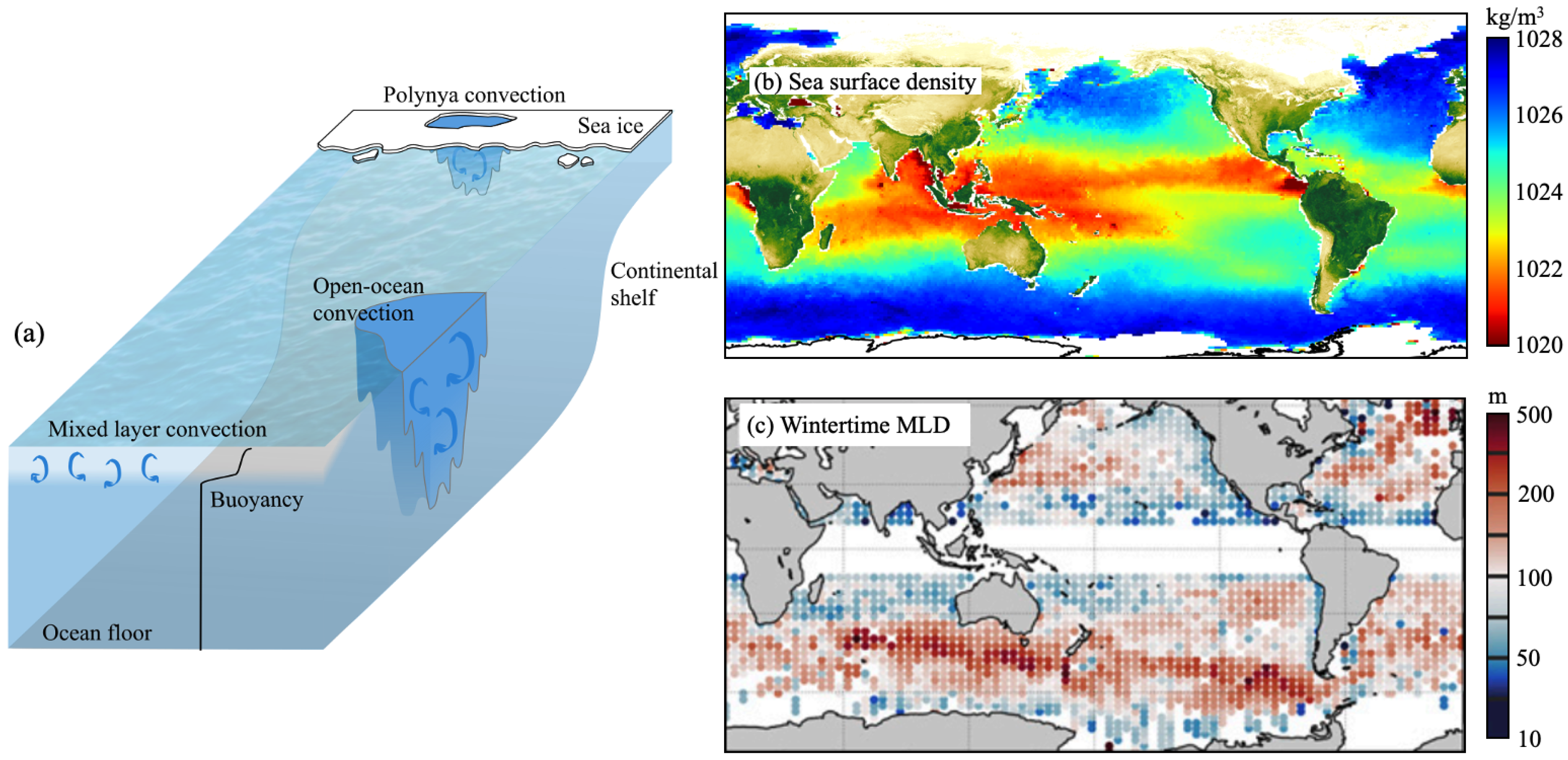
Figure 1.
(a) Schematic of different types of ocean convection forced by surface buoyancy loss: mixed layer convection, open-ocean convection and polynya convection (shown for a coastal polynya). (b) Sea-surface density from monthly average March data (image generated using dataset from NASA Aquarius project [8]). (c) Wintertime mixed layer calculated from 2010–2019 Argo floats in February (Northern Hemisphere) and August (Southern Hemisphere) using the method outlined by Huang et al. [9], which excluded equatorial regions below 10° latitude [7]. Panel (c) is reproduced with permission from Dong et al. [7] ©American Meteorological Society.

Figure 2.
Mixed layer convection from observations taken in the North Pacific Ocean. A vertical turbulence profiler and shipboard meteorological sensors took the data over a five day period in March 1987. (a) Surface buoyancy flux primarily consisting of day-time heating (red) and night-time cooling (blue). (b) Potential temperature shown relative to the individual profile mean to better display the vertical structure. Additionally included is the averaged vertical profile, taken at the time interval shown by the vertical bars at the top and bottom of the main panel. (c) Viscous dissipation rate of turbulence kinetic energy. Additionally included is the averaged profile with the vertical blue line showing the mean of the surface buoyancy flux. The small white dots in the depth-time panels show the mixed layer depth measured using the individual profiles. Reproduced with permission from Moum et al. [1], published by Elsevier 2019.

Figure 3.
Fine-scale simulations show the three different stages of open-ocean convection. A background stratification is imposed on the initial buoyancy profile to model the ocean stratification. The dotted lines outline the horizontal extent of the destabilizing buoyancy imposed at the top surface. Colored panels show the normalized horizontal velocity (speed) and buoyancy. Note that the domain height has been stretched to more clearly show the convection dynamics, the domain height-to-width ratio is 0.025. The non-dimensionalized simulations have governing parameters which were chosen to ensure that the simulations were in the same dynamical regime expected for the ocean. Image adapted from simulations by Sohail et al. [70] and we refer the reader to this paper for further information.

Figure 4.
The squared buoyancy frequency for two Argo floats in (a) the Labrador Sea and (b) south of Greenland for the time period 2006–2008. The white line shows the mixed layer depth and the vertical lines at the top of the figures show the timing for each vertical profile. Reproduced with permission from Våge et al. [59], published by Springer Nature 2009.
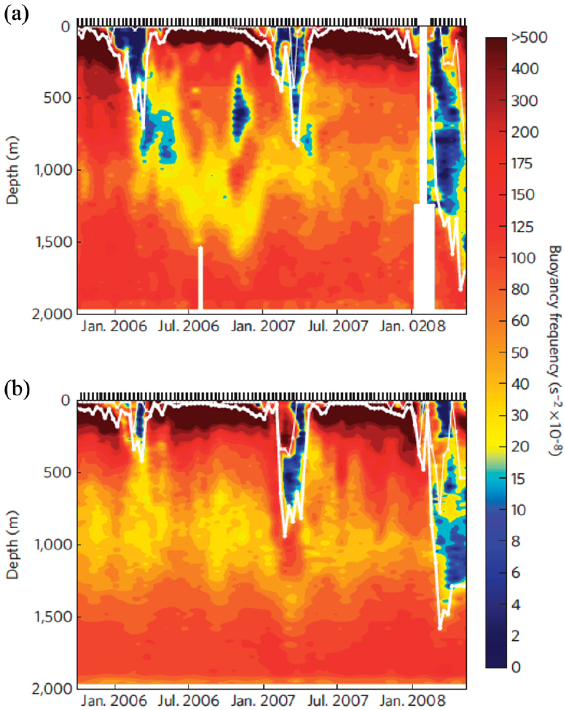
Figure 5.
(a) The surface freshwater flux in the Southern Ocean for March–September (wintertime). Note that the wintertime surface buoyancy flux is dominated by the surface freshwater flux in this region. The sea-ice sector is the colored region partitioned to the north by the bold black line. The surface freshwater flux is shown here in units of equivalent W/m2 (i.e., units of surface heat flux). The flux data are from analysis of ocean observations beneath sea-ice from ships, floats, drifters, and seal instruments [108,109]. Reproduced with permission from Pellichero et al. [109], published by Springer Nature 2018. The green dot shows the location of the Adélie Land observations in (b,c). (b) Satellite photograph of the coastal polynya and mooring position (green dot) off the coast of Adélie Land. (c) Mooring data of potential density of the water column at various depths (indicated by color, all depths are in meters). Both (b,c) are reproduced with permission from Snow et al. [95], published by John Wiley and Sons 2018.

Figure 6.
Schematic of different types of convection covered in this review, in terms of typical latitudes and time scales. Color opacity indicate where that type of convection is more common (darker) or less common (lighter). The solid line borders show the outer values that may reasonably see some occurrence of the convection type. The latitude shown is the absolute value, in other words the schematic holds for both the Northern and Southern Hemispheres. Note that open-ocean convection is mainly observed in the North Atlantic Ocean and polynya convection is strongest in the Antarctic regions.

Publisher’s Note: MDPI stays neutral with regard to jurisdictional claims in published maps and institutional affiliations. |
© 2021 by the authors. Licensee MDPI, Basel, Switzerland. This article is an open access article distributed under the terms and conditions of the Creative Commons Attribution (CC BY) license (https://creativecommons.org/licenses/by/4.0/).
Share and Cite
MDPI and ACS Style
Vreugdenhil, C.A.; Gayen, B. Ocean Convection. Fluids 2021, 6, 360. https://doi.org/10.3390/fluids6100360
AMA Style
Vreugdenhil CA, Gayen B. Ocean Convection. Fluids. 2021; 6(10):360. https://doi.org/10.3390/fluids6100360
Chicago/Turabian StyleVreugdenhil, Catherine A., and Bishakhdatta Gayen. 2021. "Ocean Convection" Fluids 6, no. 10: 360. https://doi.org/10.3390/fluids6100360