1. Introduction
The governing equations that describe the dynamics of simple fluid systems upon motion under isothermal conditions include mass and momentum conservation equations. For incompressible fluids, they may be written as
where
is the velocity vector,
is the pressure,
g is the gravity,
is the density and
is the kinematic viscosity [
1]. Solutions of the above two equations can describe large spectra of flow conditions, including both laminar and turbulent flows.
A number of simplified versions of the above equations can be established that suit different flow conditions [
2]. One such simplification is associated with creep-type flows in which fluids are moving so slowly such that their inertia may be neglected. In this case, the above momentum equations become linear, which facilitates the solution. In the more general case in which fluid inertia may not be neglected, and two categories of flow conditions may be identified according to the Reynolds number. Therefore, when the Reynolds number is relatively small such that the flow is laminar, the solution, which, in most cases, will be acquired numerically, may, generally, be easier to obtain.
This would not be the case when the Reynolds number is large, and the flow is turbulent. Although the above equations are still valid, their solution would be a challenge because of the highly nonlinear character of the momentum equation. In order to capture the flow field, one would need to consider spatial and time resolutions on the order of the smallest length and time scales associated with the flow field. These smallest length and time scales are related to the Kolmogorov smallest scales at which viscosity dominates, and the turbulent kinetic energy is dissipated into heat.
Both the Kolmogorov length and time scales are, respectively, defined as
and time scale is
, where
is the average rate of dissipation of turbulent kinetic energy per unit mass, and
is the kinematic viscosity [
3]. These scales are dependent on the flow conditions, and, for typical turbulent flows in pipes, they can prove to be very small. In other words, for a typical turbulent flow conditions in simple geometries, solutions would require exhaustively larger computing infrastructure to solve even simple scenarios.
The question now is that, do we really need such detailed information about the flow system for the sake of our engineering design? The answer to this question is likely no. Even if we have such details about the flow field, we must integrate them into a lesser number of flow parameters that are crucial for design purposes. This implies that a certain level of upscaling may be required to integrate variables so that the upscaled variables are useful in applications. Such upscaling may be done either with respect to time or space dimensions or both.
Spatial upscaling is useful in reducing the dimensionality of the problem or for constructing multitudes of overlapping continua [
4,
5,
6]. Time upscaling, on the other hand, homogenizes time-varying parameters and generates smoothly, time-varying upscaled parameters. In turbulent flows, we are not usually interested in spatial homogenization. Rather, it is the homogenization over time (sometimes is called time-averaging) that is required [
7]. Equations (3) and (4) show typical spatial and time averaging (filtering) operations, respectively.
where
is any variable (which could be scalar, vector, or tensor),
x is the position vector,
r is the position vector emanating from the centroid of the averaging volume,
V is the averaging volume, and
T is the averaging time interval.
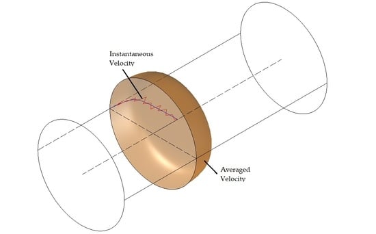
Figure 1 shows a schematic of the averaging volume along with the position vectors
x and
r.
There are, however, certain rules that need to be followed in choosing the appropriate averaging time interval. These are: (1) the averaging time interval must be much larger than the time period over which small-scale variations occurs, and (2) it must be much smaller than the macroscopic time scale (e.g., the time for concluding an experiment). Such averaged quantities are then implemented into the governing equations with the hope that new equations in terms of only the averaged parameters are developed. Unfortunately, this is not the case, and small-scale variables also appear in the governing equations. These terms need to be modeled in terms of averaged quantities in order to close the developed equations [
7]. In index notation, the upscaled momentum equation may be written as
where
is the averaged velocity,
is the averaged pressure,
is the averaged body force, and
is the fluctuating velocity. The comma in the above equation represents spatial derivative in the direction of the corresponding index.
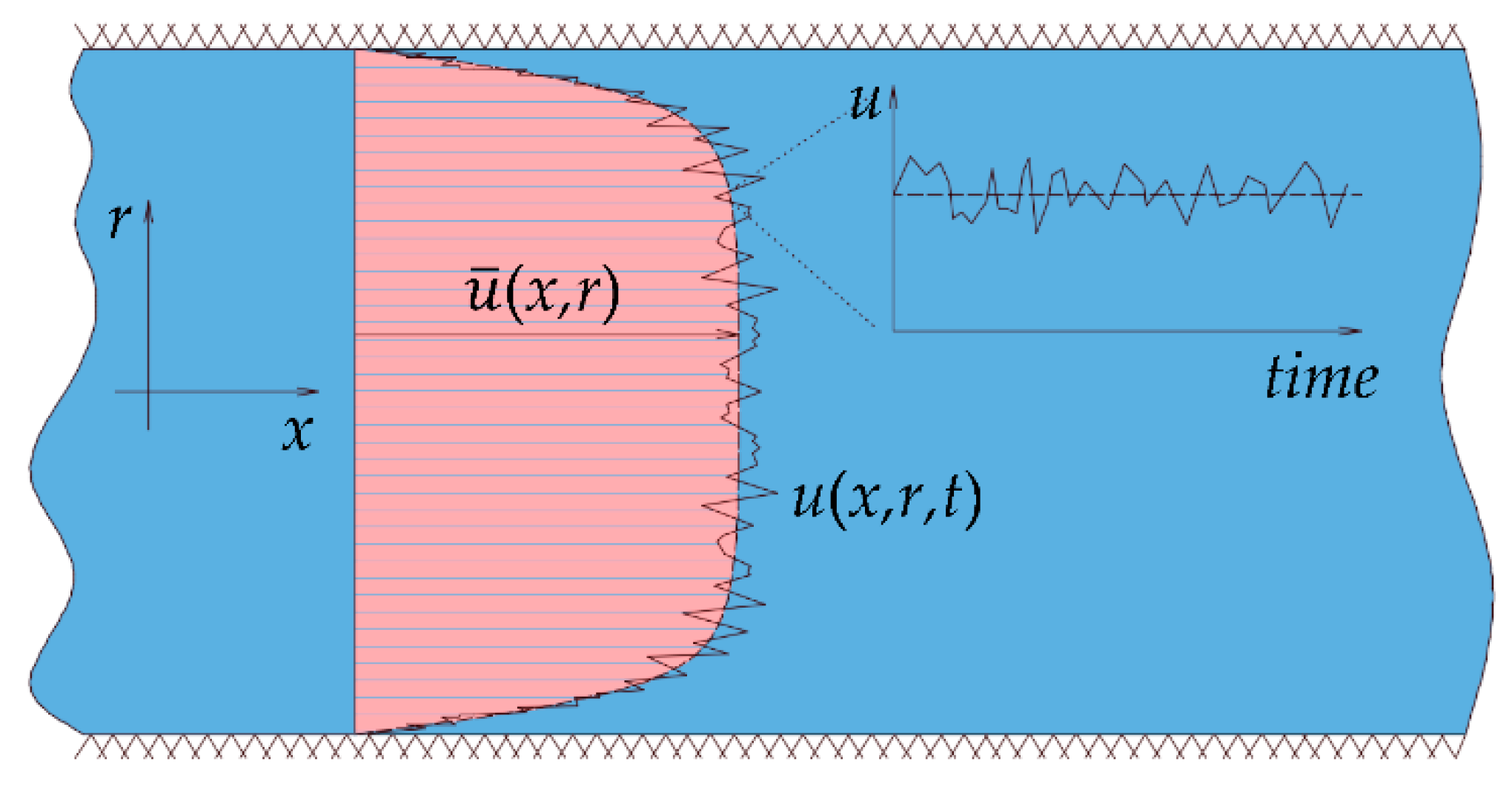
Figure 2 shows a schematic of the average velocity profile and a snapshot of the transient profile. The above equations are sometimes referred to as the Reynolds Averaged Navier Stokes (RANS) system.
The left-hand side of Equation (5) represents the change in the mean momentum of a fluid element owing to the unsteadiness in the mean flow and the convected momentum by the mean flow. This change is balanced by the mean body force, the mean pressure field, the viscous stresses, and apparent stress owing to the fluctuating velocity field. This nonlinear Reynolds stress term requires additional modeling to close the RANS equation for solving and has led to the creation of many different turbulence models.
With all the simplifications gained by appealing to RANS (Equation (5)) rather than the primitive conservation equations (Equations (1) and (2)), the most significant advantage may probably be the substantial reduction in the number of degrees of freedom that need to be considered. Despite this important achievement, the need for solving RANS for simple but ubiquitous flow problems, like flows in pipes or in channels, remains cumbersome. One of the parameters that need to be determined in such cases may be the wall shear stress in addition to the flow rate.
In other cases, it may not even be important to have information other than a few macroscopic parameters for the sake of our design practices, such as the cross-sectional average velocity. In this case, it suffices to establish a realization of the velocity profile that adheres to most of the stipulations pertinent to the characteristics of the flow (e.g., the no slip conditions at the walls, symmetry, and continuity). Even though an equation for establishing such a velocity profile may not be determined from the basic RANS, experimentation suggests the existence of such a profile.
There have been two approaches for establishing expressions that describe the velocity profile for turbulent flows in pipes. While the emphasis of the first approach has been on determining the shear stress at the wall, the other one has been focusing on the bulk shape of the velocity profile as depicted from experiments without the need to regenerate or calculate the wall shear stress, and both approaches serve the purposes of different applications [
8,
9,
10]. This is the topic of this research in which a generalized expression for the velocity profile that stems from the power law is developed and tested against experimental data.
2. Motivation and Background
Equation (5) depicts the upscaled momentum equation in three dimensions. It can be expanded in the direction of the flow (for a simple pipe or channel flows), and ignoring the body force, as
The three correlation terms
,
, and
are called turbulent stresses,
. As is clear, the turbulent stresses represent the influence of the small-scale variations on the upscaled variables. They are unknown a priori and must be modeled in terms of upscaled quantities so that the system of equations is closed. In pipe and boundary-layer flow, the stress
associated with direction normal to the wall is dominant (in the y-direction) [
11,
12]. In this case, the shear stress can be written as
and one can approximate, with considerable accuracy, the above streamwise momentum equation as
The categorization of the shear stress into two components, namely
and
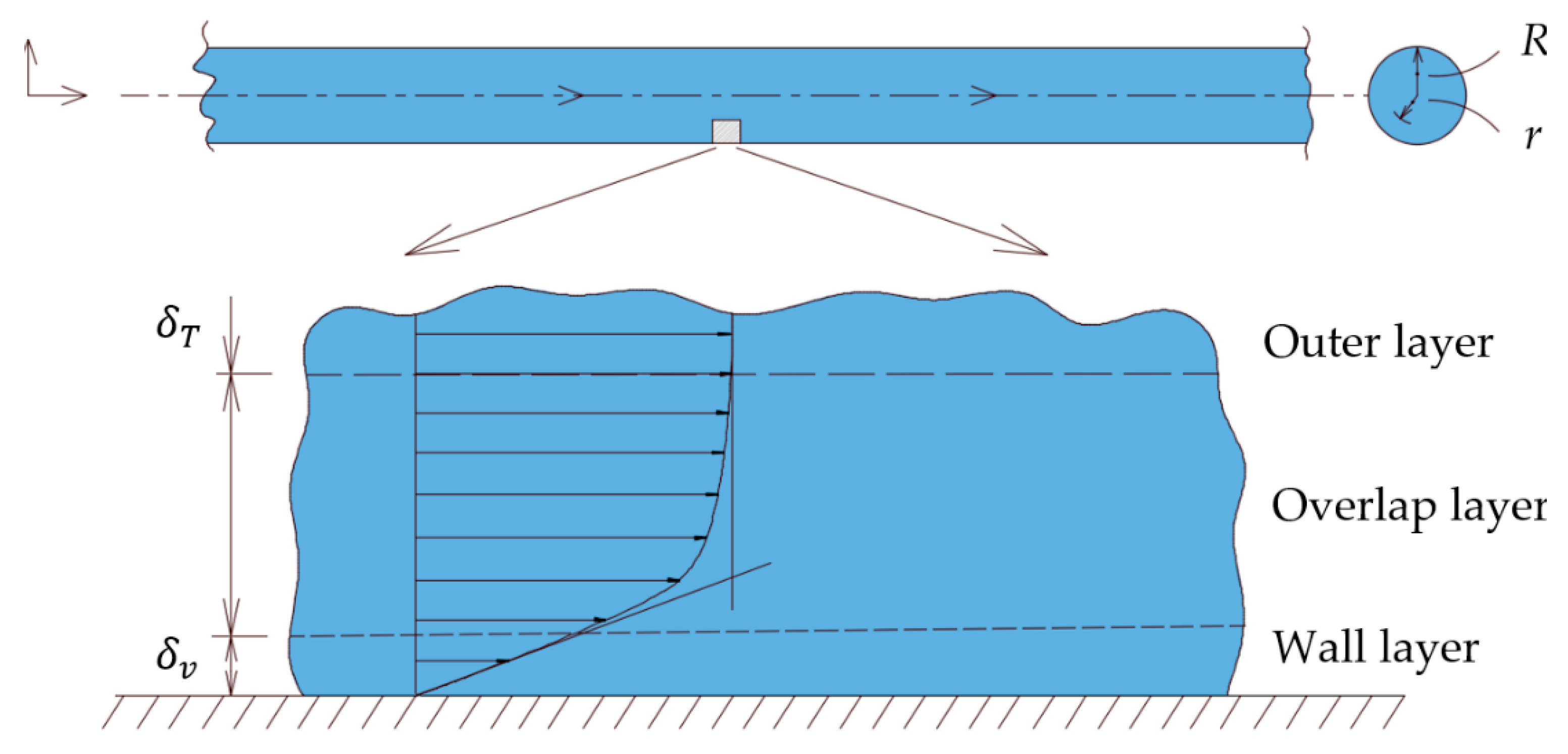
allows for the characterization of the flow field into layers according to the dominant contribution of both components as shown schematically in
Figure 3. Therefore, one can identify three layers according to the following criteria, namely:
Wall layer: in which viscous shear dominates .
Outer layer: in which turbulent shear dominates .
Overlap layer: in which both types of shears are important .
On the other hand, the previous discussion represents, to some extent, the limits to which the theoretical analysis can go in terms of simplifications. It remains, therefore, to continue the analysis via a combination of dimensional analysis and experimental observations to shed more lights into the behavior of fluids in these three layers.
Figure 3 is a schematic of the velocity profile in the near wall region along with the three designated sublayers, namely the wall layer, the overlap layer, and the outer layer.
According to Prandtl (1930) [
11], for the wall layer,
must be independent of the shear–layer thickness (where viscous shear dominates), and one can write the functional dependence of the average velocity in this layer with the flow parameters as
. Dimensional analysis introduces the following relationship
The term
is termed the friction velocity because it has the dimension of velocity, although it is not actually a flow velocity. For simplification of notation a velocity term
, is used to replace the friction velocity such that
. With substitution into the above equation, one obtains what is called the law of the wall
Experiments show that the function
may be expressed as
. Introducing the term
as a dimensionless normal distance, Equation (9) may be written as
The quantity
, which has the dimension of length, is sometimes referred to as the viscous length. For smooth surfaces, the viscous sublayer thickness,
δv, (
Figure 3), is found experimentally to be approximately five times the viscous length [
1]. This viscous sublayer gets thinner as the mean velocity increases, and the velocity profile becomes nearly flat for the cases in which the Reynolds number is very high.
In the outer layer, on the other hand, Von Karman [
13] suggested that
is independent of the molecular viscosity. However, the deviation of
from the stream velocity
Umax (sometimes is called velocity defect) should depend on the layer thickness
δT (
Figure 3) among other properties. One may, likewise, be able construct the functional dependence of this deviation as
and dimensional analysis reveals that
Even though the two laws for the velocity in the inner and outer layers look different, they must smoothly merge in the middle layer as shown in
Figure 3. Millikan [
1,
11] suggested that this can be true only if the overlap-layer velocity varies logarithmically with y such that
Approximate values for the parameters κ and B that are found to fit a wide range of turbulent flows over smooth wall are: κ = 0.41 and B = 5.0.
The previous discussion revealed how laborious it is to establish a velocity profile that satisfies considerations related to the wall shear stress. If one, on the other hand, is not interested in accurate estimation of the wall shear stress and instead only interested in the shape of the velocity profile that fits experimentations then a more reasonable approach may be to propose a mathematical relationship that may reproduce the experimentally determined mean velocity profile.
In this way, it is not guaranteed that the constructed velocity profile can adequately estimate the wall shear stress. This may be acceptable in applications that require information about, for example, the flow rates [
5,
14,
15]). In these applications, the velocity variations in the near wall region only constitute a smaller portion of the total flow rates and even if there are errors in matching the velocity field in this region, it will not considerably affect the calculations of the flow rates. In fact, it is the error in the core portion of the pipe that can result in inaccuracies in the estimation of the flow rate. This has led to establishing the very successful power law model [
16,
17,
18], which takes the form
where the exponent
n is, generally, a function of the
Re. In the above equation, the bar over the velocity, which indicates an averaged quantity, has been dropped for the simplicity of notations. In many cases, it is found that a value of
n = 7 fits many of the cases of turbulent flows over smooth surfaces. It is to be highlighted that, the previously mentioned power law (Equation (13)) is a fitting artifact and is not derived from the solution of the governing equations for the mean pipe flow, (i.e., the RANS).
However, it is appealing and widely used in several applications because of its simplicity and resemblance to that of laminar flows. Indeed, there are solutions of the RANS that offer alternatives for calculating mean pipe flows, e.g., Pai [
19], Garcia and Farinas [
20,
21,
22], and for channel flow, [
23]. In fact, Pai polynomials have shown to compare very well with the experimental data [
24].
It is, however, to be indicated that, unlike laminar flows where the shear stress at the wall is dependent on the normal to the wall velocity gradient, in turbulent flows, it is much more involved. There are two approaches to handle the calculations of shear stress at the wall in turbulent flows. In the first approach, one may use the mean velocity gradi-ent, and, in this case, additional contributions from the fluctuating stresses need to be in-corporated. Such extra components have been correlated with the mean velocity gradient via the concept of turbulent viscosity.
A relatively larger number of fitting parameters are incorporated in this process to achieve compliance with the measured shear stress. The second approach, on the other hand, which may be valid in simple geometries (e.g., pipe flows), realizes that the near wall region features multitude of length scales and is divided into subregions that may not be captured in a single mean velocity profile. Therefore, the near wall region is further resolved towards the laminar sublayer via the logarithmic law of the wall.
It comes, therefore, back to the previously highlighted point, which is, if someone is interested in determining flow rates or other flow-dependent parameters, an experimen-tally fitted power law may suffice provided that its range of applicability is enlarged. It is believed that a generalized power law that should work over a wide range of operating conditions should depend on more fitting parameters than a mere one. It should also cor-rect some of the draw backs of the one-parameter power law, which is actually the focus of this research.
3. The Generalized Power Law
In laminar-type flows in pipes, the velocity profile has been analytically determined to follow a parabolic relationship in the form
According to this relationship, the average velocity can be estimated and is found to be half the centerline velocity, i.e., . This developed parabolic velocity profile not only matches the experimentally determined profiles but can also be used to accurately estimate the wall shear stress. For turbulent-types flows, on the other hand, the experimentally fitted velocity profile widely used takes the form as given in Equation (13).
As indicated earlier, the exponent
n is, generally, a function of the
Re, however, it has been found that a value of 7 fits reasonably well the velocity profiles for fully developed turbulent flows. This law, however, has two main drawbacks, namely (1) it does not have continuous derivative at the centerline (the derivative
is nonzero), and (2) it does not reduce to the laminar flow profile when the
Re is relatively small. This motivates us to consider a generalized power law that covers the whole spectrum of flow conditions including both laminar and turbulent flows. It takes the general form
where
m and
n are exponents that tolerates the generated profile to match the experimentally determined profiles. Equation (15) reduces to the laminar velocity profile (Equation (14)) when
m = 2 and
n = 1 for lower
Re. This implies that the exponent
n is, likewise, correlates with the
Re and it is 1.0 for laminar flows. We further investigate the continuity of the derivative of the velocity at the centerline. For simplicity of the notation, let
and
; therefore, when
r = 0 (i.e., at the centerline),
, and when
r = R (i.e., at the wall),
. The above equation becomes
When
m = 1 (which corresponds to the traditional power law),
is
Two discrepancies are associated with this presentation of the velocity profile as noted by Ŝtigler [
25]. These are, namely (1) when
(i.e., at the centerline), the derivative is nonzero
, which implies that the velocity profile experiences jump in the derivative at the centerline, and (2) at
(i.e., at the wall),
.
On the other hand, when
, the derivative of Equation (16),
, is
In this case, when
(i.e., at the centerline),
, which resolves the first discrepancy; however,
still approaches infinity near the wall. This does not appear to pose a significant problem on account for the fact that such a velocity profile is not going to be used to estimate the shear stress at the wall, as discussed in the previous section. It is to be noted that Peszyński et al. [
26,
27] proposed that the parameter
m should take a value of 2 if continuity of the derivatives at the centerline is to be maintained. In this work, we investigate the optimum values of the parameters
m and
n such that good fitting of the experimental data is obtained.
Extensive comparisons with published benchmark setup and CFD analysis are conducted to establish ranges for the two parameters m and n. Furthermore, analysis of these two parameters will also be considered to choose those values of the two parameters that maintain continuity of the derivative at the centerline. The values of the two parameters are determined following optimization exercises to minimize the sum of square deviation as will be discussed later.
4. Sensitivity Analysis
In this section, we provide sensitivity analysis on the effects of the two parameters
m and
n on the behavior of the model. As indicated earlier, the velocity profile should fulfill the continuity of the derivative at the centerline. This is fulfilled for the cases in which
. In other words, at the centerline, when
m = 1 (which corresponds to the well-known power law), the derivative of the velocity with the radius (i.e.,
) experiences discontinuity. This is depicted in
Figure 4, which shows that the slope of the velocity profile at the centerline is nonzero.
Figure 5 shows the normalized velocity profile along the radius of the pipe for the newly proposed model. In particular, it shows the sensitivity of the model to the parameter
m for fixed value of the exponent
n (
n = 7). Values of the exponent
m considered are 2, 3, 4, and 6. As shown, the discontinuity in the derivative of the velocity at the centerline has vanished. However, the range of variations of the velocity profiles from the laminar case to the turbulent cases does not show possibilities to cover the transition zone with the smallest value of
m taken as 2.
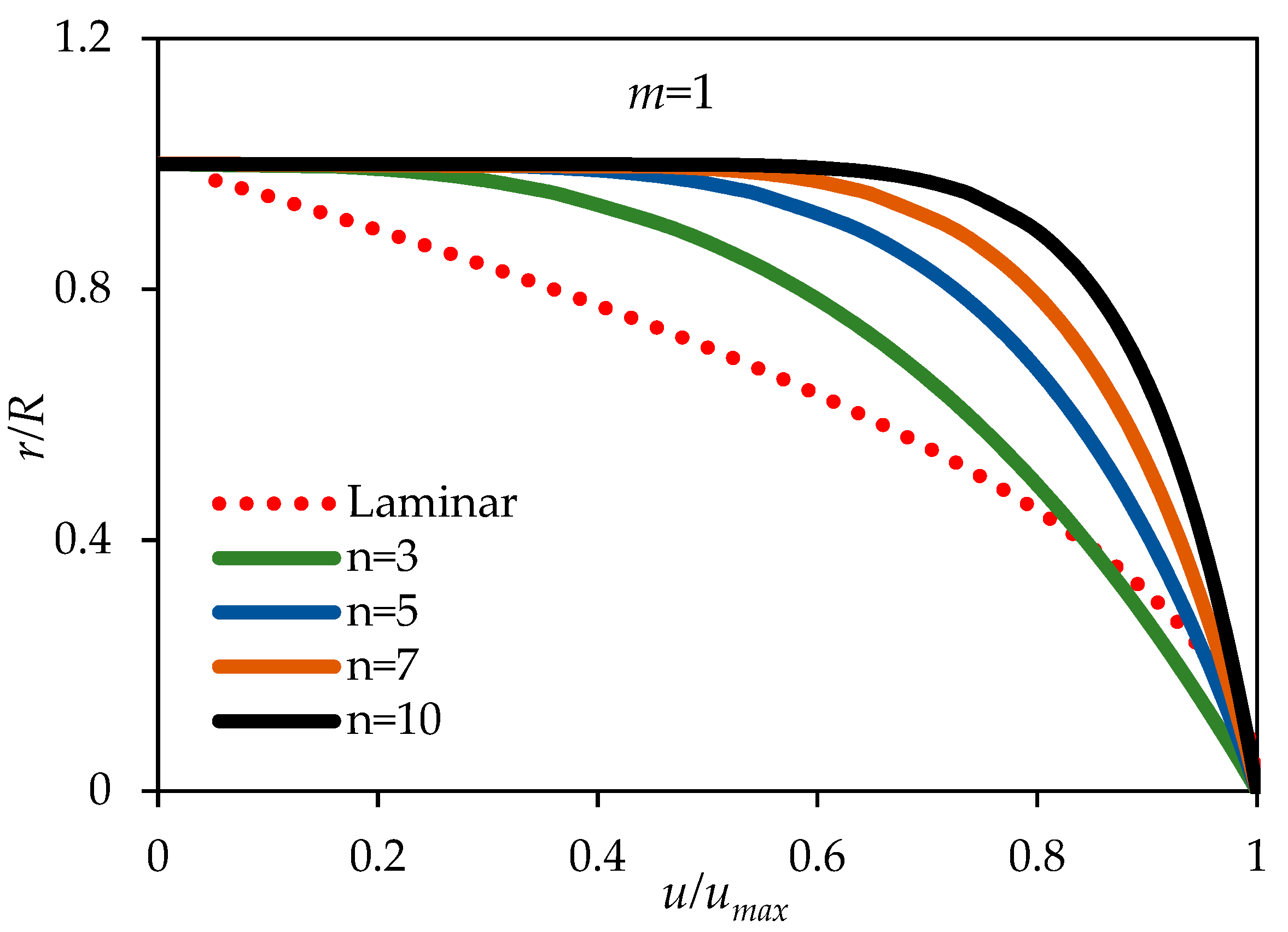
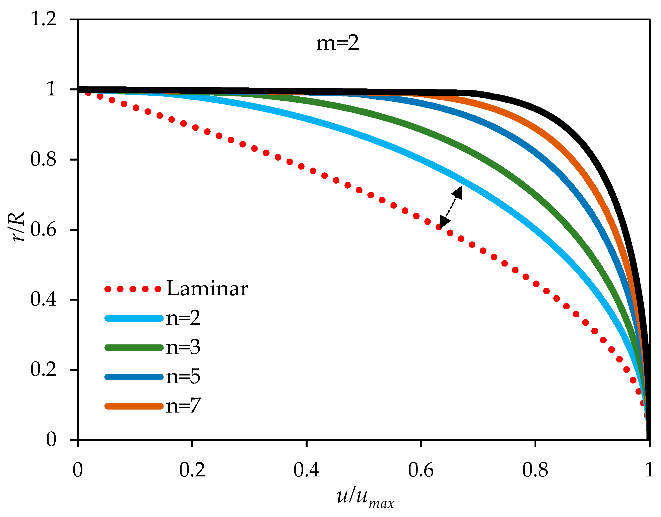
Figure 6, on the other hand, shows the sensitivity of the model to the variations of the parameter
n for a fixed
m. The value of
m considered in this example is 2 such that the model reduces to the laminar profile for the case in which
n is unity. The values of
n considered in this example include 2, 3, 5, 7, and 10. As depicted in the figure, the derivative of the velocity with radius at centerline is continuous. Furthermore, the model seems to cover a wider range, including possibly the transition zone by changing the exponent
n. It is, therefore anticipated that a value of the exponent
m of 2 may fill in the spectrum of velocity profiles over a wider range of
Re. It remains important to provide comparisons with experimental data and/or CFD studies to build confidence in the new model.
The previous discussion indicates that a proposed variation of the exponent
n over a wider range of
Re for the case when
m = 2 may be schematically displayed as shown in
Figure 7. In this figure, the value of
n in the laminar region is constant and equals one. In the fully turbulent region,
n increases in a nonlinear fashion at relatively smaller
Re then at a slower pace at higher
Re. In the transition region, on the other hand, the value of
n is expected to increase with the
Re in a faster pace to merge the two regions.
In this work, we show how the parameter
n varies with the
Re, via comparisons with the experimental data. Since, to the author’s knowledge, there are no reported measurements of the mean velocity profile in the transition region, there will be no indication on how the parameters
m and
n change within the corresponding range of
Re.
Figure 7 is just an illustration on the expected behavior of the parameter
n with
Re. In the comparisons section, the actual dependence of the parameters
m and
n with
Re is displayed.
5. Comparisons with Experiments and CFD Analysis
In this section, comparisons with experimental and CFD works of some benchmark published works are reported. We first start with the reported data of the carefully designed and calibrated experimental setup constructed in the Gas Dynamics Lab at Princeton University. Following this, we also provide comparisons with the experimental and CFD works of Odewole et al. [
28].
The SuperPipe facility at Princeton University is designed to investigate fully developed turbulent pipe flows over a wide range of Reynolds numbers. Air is used as the working fluid at pressures up to 3500 psi. The SuperPipe has an internal diameter of 5.09 in with a length to diameter ratio (L/D) on the order of 200 to achieve fully-developed flow conditions. The pipe is made with a smooth-wall finish (roughness < 6 µm). The setup allows very accurate measurements over a large range of Reynolds numbers, (approximately from 5 × 10³, to about 3.8 × 10⁷).
Details of the facility can be found in Zagarola [
29]. In addition to the data set and analysis presented by Zagarola [
29], Zagarola and Smits [
30], and Zagarola et al. [
31], in this work, we use the data set of McKeon et al. [
32,
33] who reported the measurements of the mean velocity profiles in fully developed turbulent pipe flow. They used a smaller Pitot probe to reduce the uncertainties due to velocity gradient corrections. In addition, they reported using a new static pressure correction in analyzing all data (around 25 profiles altogether).
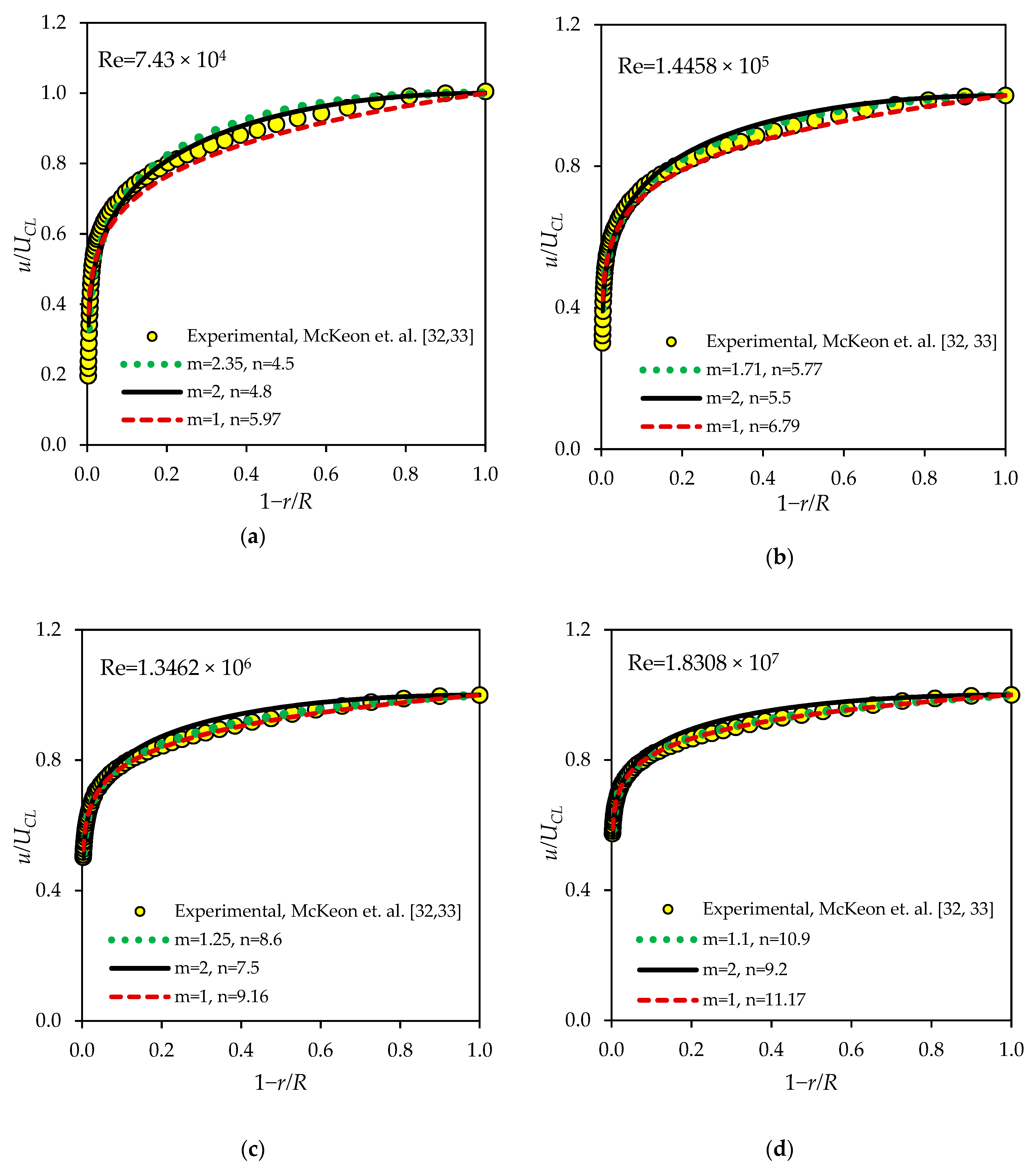
We compare between the measured velocity profiles and three scenarios of the two parameters m and n. In the first scenario, both m and n are optimized to fit the experimental data by minimizing the sum of square deviations (SSD), with , where is a measured quantity and is its calculated counterpart. In the second scenario, m is considered equals 2, and the parameter n is optimized. In the third scenario, likewise, the parameter m is set equal to one, and the n is optimized.
Such exercises were conducted over 17 velocity profiles of which four representative comparisons of velocity profiles at different
Re and for different combinations of
m and
n are shown in
Figure 8a–d. In
Figure 8, the normalized axial velocity (normalized by the centerline velocity) is depicted against the normalized distance from the centerline (normalized by the radius of the pipe) for different Reynolds numbers. As is clear, the larger the
Re number, the velocity profile is flattened, which is a manifestation of increased turbulence.
The velocity profiles represented by the green dotted lines (which are obtained by optimizing both
m and
n) are closer to the measured profiles than the other two scenarios. Furthermore, it can be seen that, in this scenario, the parameter
m changes over a relatively smaller margin as compared with the parameter
n. This is also depicted in
Figure 9a–c, which shows the variations of the two parameters
m and
n with
Re for the three scenarios.
Figure 9d reports the minimized SSD for the three cases.
Figure 9a shows the changes of both
m and
n over a range of
Re that extends from laminar flows to turbulent ones with both
m and
n optimized. Likewise,
Figure 9b depicts the second scenario in which the parameter
m in the turbulent region is set fixed to a value of 1.0 while the parameter
n is optimized by minimizing the SSD. This scenario represents the traditional power law. The third scenario depicts the optimization of the parameter
n with the parameter
m set to 2.0 in the turbulent region (
Figure 9c), which represents the modified power law suggested by Peszyński et al. [
26,
27]. The minimized SSDs corresponding to the optimized
n for the three scenarios are shown in
Figure 9d.
It is seen from the figure that, for larger values of Re, the three scenarios result in a smaller SSD, which implies good fitting. The best fitting, however, over the whole spectrum of Re, in the turbulent region, is that corresponding to optimized m and n values. However, since the parameter m changes over a smaller range, it is reasonable to take a fixed value of m to represent the whole range. A value of 2.0 for the parameter m not only maintains the continuity of the derivative at the centerline but also reduces to the laminar profile when n is 1.
In addition to comparing with the SuperPipe benchmark, comparisons with other datasets available in literature were also conducted. Odewole et al. [
28] performed an experimental study to construct the velocity profile inside a pipe of approximately 9 m in length and 10 cm in diameter. They used a hot-wire probe to measure the velocity across the pipe in the fully turbulent region (
Re = 6800). Furthermore, they calculated the mean velocity profile numerically using the
k-ε model and obtained a very good match.
We compare the computed velocity profile using our generalized power law model with their measurements and CFD results to build confidence in the presented model and to suggest optimum values for the two exponents
m and
n.
Figure 10 shows a comparison between measured velocity profiles by Odewole et al. [
28], and the calculated profiles for the cases in which
m takes the values 1, 2, 3, and 4, respectively, with
n taken as 7. The velocity profile corresponding to the case in which
m = 1 and
n = 7 refers to the known one seventh law of the wall and that corresponding to
m = 2 refers to that proposed by Peszyński et al. [
26,
27].
As
Figure 10 depicts, the known law of the wall underestimates the velocity across the section of the pipe. Furthermore, it does not approach the centerline velocity with a slope that approaches zero. In other words, there would be a discontinuity in the first derivatives of the velocity.
Figure 10 also shows that, when
m is taken to be 2 or 3, the calculated velocity profiles match reasonably well with the measured one. When
m is taken to be 4, the calculated velocity profile slightly overestimates the velocity when compared with the measured one.
Figure 11, on the other hand, depicts comparisons between the measured, computed using CFD analysis, and computed using the proposed generalized power law velocity profiles. Two values of the exponent
m have been used, namely 2 and 3. As shown, the new power law with values of
m taken as 2 and 3, and
n taken as 7, shows excellent matches with both the measured and calculated velocity profiles. While
Figure 11 shows a good match in the turbulent core region, it is not clear how the comparisons perform in the near wall region.
To highlight the comparison in the wall region, the error between the measured profile and the power law profiles is shown in
Figure 10. The error is calculated as
where
is the percentage error,
is the measured velocity, and
is the calculated one.
Figure 12 shows the error function for the cases when
m takes the values 1, 2, and 3. Clearly, the error is less in the core region for the cases when
m is taken as 2 and 3, whereas it is relatively large in the near wall region. Furthermore, the error for the case when
m is one (i.e., the traditional power law) the error is relatively large in both the core and the near wall region.
This suggests that the newly developed power law is more accurate than the older counterpart. Moreover, both laws fail in the near wall region as explained earlier. Needless to say, working with power law is not going to be used in the calculation of the wall shear stress. It is only useful in determining quantities like the flow rates where the wall region has negligible influence compared with the core region in the calculations of the flow rates in fully turbulent flow.
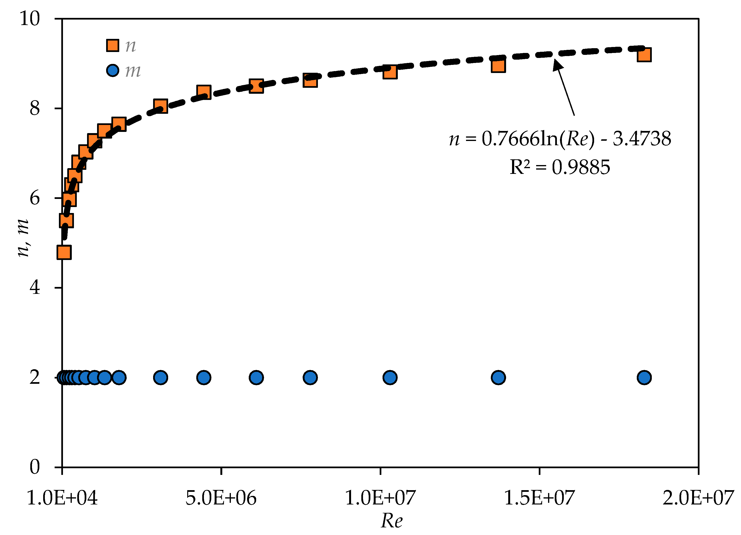
The previous discussion and comparisons suggest that a new power law velocity profile that covers a wider range of Re would be one that incorporates two fitting parameters as given in Equation (15). With the parameter m varying over a smaller range, it may be possible to lump it into a single value that spans the whole spectrum of Re. A value of 2 seems reasonable as it maintains the continuity of derivatives and reduces to the laminar profile for smaller Re.
The variations of the parameter
n with
Re, as depicted in
Figure 9a–c, for the three scenarios can be used to establish correlations that relate
n and
Re. As we have reached the conclusion that a value of 2.0 is suitable for the exponent
m over the whole range of
Re, we choose this scenario to establish the desired correlation between
n and
Re.
Figure 13 shows the variations of the exponent
n with
Re (on a linear scale) in the turbulent region. As can be seen, a logarithmic equation fits the experimental data (in the range of
Re between ~1 × 10
4 and 2 × 10
7) very well with R
2 = 0.9885. The correlation takes the form:
The cross-sectional average velocity, therefore, may be calculated as
where
is the beta function (also called the Euler integral of the first kind). This above equation is valid for the case in which
. Substitution with the values of
m and
n as 2 and 7, respectively, one obtains
Finally, similar formula may also be developed for noncircular ducts (e.g., rectangular and other rounded ducts), such as those investigated by Peszyński et al. [
27]. However, because of the lack of extensive experimental data that covers larger spectrum of
Re, it is not possible to provide such analysis on the optimized parameters
m and
n as those established in this study for circular pipes.


