
A CFD Tutorial in Julia: Introduction to Compressible Laminar Boundary-Layer Flows


School of Mechanical and Aerospace Engineering, Oklahoma State University, Stillwater, OK 74078, USA
*
Author to whom correspondence should be addressed.
Fluids 2021, 6(11), 400; https://doi.org/10.3390/fluids6110400
Submission received: 13 October 2021
/
Revised: 30 October 2021
/
Accepted: 2 November 2021
/
Published: 5 November 2021
(This article belongs to the Collection Feature Paper for Mathematical and Computational Fluid Mechanics)
Abstract
:A boundary-layer is a thin fluid layer near a solid surface, and viscous effects dominate it. The laminar boundary-layer calculations appear in many aerodynamics problems, including skin friction drag, flow separation, and aerodynamic heating. A student must understand the flow physics and the numerical implementation to conduct successful simulations in advanced undergraduate- and graduate-level fluid dynamics/aerodynamics courses. Numerical simulations require writing computer codes. Therefore, choosing a fast and user-friendly programming language is essential to reduce code development and simulation times. Julia is a new programming language that combines performance and productivity. The present study derived the compressible Blasius equations from Navier–Stokes equations and numerically solved the resulting equations using the Julia programming language. The fourth-order Runge–Kutta method is used for the numerical discretization, and Newton’s iteration method is employed to calculate the missing boundary condition. In addition, Burgers’, heat, and compressible Blasius equations are solved both in Julia and MATLAB. The runtime comparison showed that Julia with loops is 2.5 to 120 times faster than MATLAB. We also released the Julia codes on our GitHub page to shorten the learning curve for interested readers.
1. Introduction
Until the 19th century, scientists neglected the effects of viscosity in their hydrodynamic and aerodynamic calculations using potential flow theory. However, this assumption led to a contradiction between theoretical predictions and experimental measurements of drag force acting on a moving body, now known as the d’Alembert paradox [1]. Later, a revolutionary boundary-layer concept is introduced [2,3]. In this concept, the fluid flow over a surface is divided into two regions by the boundary-layer edge: an area between the surface and the boundary-layer edge dominated by the viscous effects and a region outside the boundary-layer edge where the viscous effects can be neglected. It enables a significant simplification of full Navier–Stokes equations.
The boundary-layer theory was first presented by Prandtl [4] in 1904, and it provides the solutions of velocity and temperature profiles within the boundary-layer by using approximations. One can obtain Blasius [5,6], Falkner–Skan [7], and compressible Falkner–Skan [2,8] solutions by using this approach. Researchers extensively use these solutions to validate the computational fluid dynamics (CFD) simulations. Moreover, in a CFD simulation, one can calculate the boundary-layer thickness in advance to estimate the required grid parameters to resolve the boundary-layer region. Understanding the fundamentals of boundary-layer theory is critical for engineers to solve today’s aerodynamic design challenges.
It may be challenging to fully understand the fundamentals of the boundary-layer theory in undergraduate- and graduate-level boundary-layer courses. Most of the time, books skip or briefly mention some steps in the derivation of a system of equations. Additionally, instructors are forced to leave the details of derivations to students due to the limited lecture time. The steps that are skipped may become a challenge for students. Moreover, the derived equations usually do not have an analytical solution; therefore, they must be solved using numerical methods. Students or engineers who do not have adequate experience in the subject may struggle to understand the details of the topics because of the blanks in the process. A tutorial of step-by-step derivation and implementation in the computer environment may help students to fill the blanks. Moreover, researchers from another field may utilize the code and/or the simple explanation of the topic in their research. For the coding part, there are several available coding languages extensively used in scientific community, such as Fortran [9], Python [10], C/C++ [11], and MATLAB [12]. However, Julia [13] may be another alternative for students to write high-level, generic code that resembles mathematical formulas. It is a relatively new, fast, and dynamic coding language that focuses on productivity. It is trying to fill the gap between high-performance languages, such as Fortran and C/C++, and user-friendly languages, such as Python and MATLAB. Students tend to use user-friendly languages for their coursework and simple problems; however, in the industry, it is crucial to have a fast solver. In this gap, Julia provides easy syntax, as Python and MATLAB, and a fast performance, as Fortran and C/C++. This makes Julia a great choice for researchers due to the ability to combine high-performance with productivity. Although there are some tutorial papers and modules developed in other languages [14,15,16,17], the current number of publications is not enough to gain a thorough understanding of the Julia language in CFD [18,19].
In this tutorial paper, compressible Blasius equation and energy equation are derived from scratch and implemented in the Julia environment. The fourth-order Runge–Kutta method is employed to solve the final differential equations and Newton’s iteration method is used for the missing boundary condition. Solutions obtained by the code are validated with Iyer’s [20] BL2D boundary-layer solver which is used in NASA’s well-known compressible boundary-layer stability solver Langley Stability and Transition Analysis Code (LASTRAC) [21]. The derivation details with the numerical implementation will guide students to understand the compressible laminar boundary-layer concept better. It will be easier for them to solve more complex problems with their own codes. Figure 1 illustrates the visual abstract of the paper, which gives the main ideas of the present paper. Additionally, Burger’s, heat, and compressible Blasius equations solution times obtained by Julia and MATLAB solvers are compared with each other. We make all these codes available on GitHub to shorten the learning curve. We provide the GitHub link of the codes, installation instructions, and required packages in Appendix A. Advanced boundary-layer topics are beyond the scope of this paper, interested readers are referred to additional references [22,23,24,25] for subsonic boundary-layer transition, references [26,27,28,29,30,31,32,33,34] for supersonic/hypersonic boundary-layer transition, and references [35,36,37] for flow separation. The other research studies where boundary-layer flow is involved are presented in the references [38,39,40,41,42,43].
2. Compressible Laminar Boundary-Layer
Compressibility effect in the boundary-layer requires additional calculations. Constant density assumption in incompressible speeds is no longer valid for the compressible boundary-layer. In compressible speeds, temperature and density change within the boundary-layer. It is crucial to capture the velocity, temperature and density variations in the boundary-layer to obtain accurate simulation results. One can estimate the number of element required to resolve the boundary-layer in the CFD simulation by using the boundary-layer theory. Compressible Blasius is also widely used for CFD validations in high-speed flows. In this section, compressible Blasius equations will be derived from scratch and implemented in the Julia environment. The contribution of this paper is employing the Julia language. The equations used in this paper are already in the literature [2,44]. The manuscript may enable students to adopt the programming language with easily and available GitHub codes, which may shorten the learning curve.
2.1. Compressible Blasius Equations
Incompressible Blasius solution is a similarity solution for a flat plate. The assumptions for the incompressible Blasius equations are given in our previous work [19]; interested readers can check the details from there. In the compressible region, the temperature effects must be taken into account for an accurate solution. In the incompressible region, the temperature and density changes are small enough to be neglected. In the compressible region, the temperature can increase drastically as a result; density decreases within the boundary-layer. For example, the temperature on the solid wall can reach 7 times the freestream temperature in Mach 6 flow over a wedge. If the freestream temperature is 300 K, the wall temperature will be around 2100 K. In order to compare the quantity, the melting point of titanium is around 1941 K [45]. This problem is still a challenge for aerospace applications in which high Mach numbers are involved.
The compressible Blasius equations can be derived from the compressible Navier–Stokes equations, which can be expressed in two spatial dimensions as:
where is the density, u and v are the velocities in x- and y- directions, p is the pressure, is the dynamic viscosity, is the second viscosity coefficient, k is the thermal conductivity, T is the temperature, is the specific heat at constant pressure, and is the dissipation function, which can be written as:
In order to obtain the boundary-layer equations, dimensional analysis is required to neglect the variables that have smaller orders than others. The flat plate boundary-layer development is illustrated in Figure 2. In this flow, u velocity is related to freestream velocity and the order of magnitude is one. The x is related to plate length, so its order of magnitude is also one. The y distance is related to boundary-layer thickness, so it is in the order of which is the boundary-layer thickness. The density, , is related to freestream density so its order of magnitude is also one. The magnitude of the v velocity can be calculated from the continuity equation, Equation (1). In order to get zero from this equation, all variables must be in the same order so v is in the order of as a result of this, . When the magnitude analysis is completed in the same manner, the boundary-layer equations can be obtained. It has to be noted that dynamic viscosity is in the order of , pressure and temperature are in the order of one. The specific heat at constant pressure is in the order of one. The second viscosity coefficient, , can be taken as because of Stokes’ hypothesis. Once the order of magnitude is obtained for each of the terms, some of the terms can be neglected because . The final system of equations in steady-state condition () will be:
Equation (7) can be expressed at the boundary-layer edge as:
The variables are changing from the solid surface up to the boundary-layer edge. At the boundary-layer edge, they reach to freestream value for the corresponding variable and remain constant. The velocity change in the y-direction at the boundary-layer edge is zero (), because it is constant at boundary-layer edge. Equation (8) indicates that the pressure gradient in the y-direction is zero, so pressure at the boundary-layer edge equals the pressure within the boundary-layer (). Equation (10) becomes:
The velocity at the boundary-layer edge is equal to freestream velocity, which is constant in x-direction for a flat plate. In other words, edge velocity gradient in x-direction is zero (). If the equation of state is used to obtain the ratio of density and temperature as:
where R is the gas constant. It is known that , so . The final system of equations is:
where . At this point, a similarity parameter can be introduced to the system to obtain a similarity solution [46]. The similarity parameter, , can be defined as:
where . Let’s assume that the stream function is
The u and v velocities can be calculated from the stream function as:
In this step, the variables in Equation (15), u, v, , , and can be calculated. The first derivative of with respect to y and the first derivative of s with respect to x will be required for the chain rule.
It is better to note that, in calculation, relation is used. The u velocity can be calculated as:
The same procedure can be applied for v velocity as:
Once u velocity is obtained, the derivatives with respect to x and y can be calculated as:
All terms in Equation (15) are known. If the above terms are substituted into Equation (15) and the necessary simplifications are done, the final equation will be:
It has to be noted that if and , in other words, if the flow is incompressible, Equation (41) becomes an incompressible Blasius equation (). Equation (41) can be further simplified as:
where and . The momentum equation of the compressible Blasius equations is obtained in Equation (42). The energy equation of the compressible Blasius equations can be obtained with the same procedure. First of all, , , and have to be calculated. These terms can be calculated as:
When these terms are substituted into Equation (17), the new equation will be:
Equation (51) can be simplified by dividing it with , substituting Prandtl number into the equation where Prandtl number and multiplying with . The final equation will be:
where , , and . In the final system of equations, the can be calculated from Sutherland Viscosity Law [47]. The dimensional viscosity function is:
where and K. The is:
The derivative of the viscosity is also required. The derivative terms can be calculated as:
The final system of equations is:
It has to be emphasized that is a function of and the final system of equations is coupled, so they have to be solved together. The boundary conditions of the system for an adiabatic system are:
The boundary condition for the isothermal wall depends on the wall temperature. For example, if the wall temperature equals the boundary-layer edge temperature, it will be , and it will be replaced with the last boundary condition of the system. In the adiabatic boundary condition, the derivative of the temperature with respect to wall-normal direction will be 0. During the numerical procedures, the difference will be emphasized one more time.
2.2. Numerical Procedure
In this section, the compressible Blasius equation will be solved with the fourth-order Runge–Kutta method [48] and Newton’s iteration method [49]. Different methods can be used for this problem; however, we used Runge–Kutta and Newton’s method because of their extensive usage in the literature and accuracy. To start the numerical procedure, high-order differential equations can be reduced to the first-order differential equations as:
if Equations (64)–(68) are substituted into Equations (58) and (59), the final version of these equations can be written as:
The final system of equations can be written in the matrix form as:
The adiabatic boundary conditions for the system are:
The isothermal boundary conditions for the system are:
The functions can be introduced in Julia as shown in Listing 1, where is the second coefficient of the Sutherland Viscosity Law, is the temperature at the boundary-layer edge, is the Mach number at the boundary-layer edge, is the specific heat ratio, is the Prandtl number and and are the terms given in Equations (64)–(66), Equation (67), and Equation (68). In the functions given in Listing 1, only 2 parameters are dimensional, which are and . In this tutorial paper, Kelvin is the unit of both parameters. If the temperature unit is required to be different, such as Fahrenheit or Rankine, the units of and must be transformed into the new unit accordingly.

Listing 1.
Implementation of system of equations in Julia environment. There are five functions which correspond to five first-order ordinary differential equations.
Listing 1.
Implementation of system of equations in Julia environment. There are five functions which correspond to five first-order ordinary differential equations.
 |
In this paper, implementation of the Runge–Kutta method will be provided. The derivation of the Runge–Kutta method and how it calculates the function value at the next step can be checked from Reference [49]. The implementation of the Runge–Kutta method for the compressible Blasius problem can be seen in Listing 2, where N is the number of elements. It has to be emphasized that the number of node points is , which means that terms must be calculated until node. The first point is the boundary condition, so there will be N number of calculations.
The initialization and the boundary conditions can be introduced as shown in Listing 3, where is a flag for the adiabatic or isothermal condition selection and is the dimensionless wall temperature. It is nondimensionalized with , so if the temperature at the boundary-layer edge, , is 300 K and the wall temperature is required to be 150 K, must be entered as . Another important point about Listing 3 is the indices. In the derived formulations, indices start from 0. However, in both Julia and MATLAB, indices start from 1. This is the reason why indices are starting from 1 in Listing 3 boundary conditions part.
Listing 2.
Implementation of Runge-Kutta method in Julia environment. It requires four slope calculation to estimate the function value in the next node value.
Listing 2.
Implementation of Runge-Kutta method in Julia environment. It requires four slope calculation to estimate the function value in the next node value.
 |
In the system of equations, there are five equations and five boundary conditions; however, two boundary conditions are located at the end of the domain. In order to start the calculation, all values at the should be given. and in the Listing 3 are the initial guesses for the missing boundary conditions. They can be any value. Once they are introduced to the system, compressible Blasius equations can be solved. When the equations are solved with guessed initial conditions, the solution vector must satisfy the boundary conditions at the end of the domain. However, it will not converge at the first try because the guessed boundary conditions are not correct. To overcome this problem, different methods can be used, such as the shooting method, bisection method, or Newton’s iteration method. In this paper, Newton’s iteration method will be used because it is fast and it is not hard to implement. In order to use it, the algorithm needs to run with the initial guesses one time. Once the (corresponds to u) and (corresponds to T) at the end of the domain are obtained, an arbitrary small number can be added to one of the initial guesses. The algorithm can be run one more time with the new boundary condition guesses. After that, the same small number can be added to the other initial guess and the algorithm can be run one more time. After running the algorithm 3 times, there will be 3 different – pairs. It has to be noted that when the small number is added to the second boundary condition (in the third run), other boundary conditions should be equal to the value in the first run. In other words, after adding a small value in the second run, it should be subtracted in the third run. The main purpose of running three times is to determine the more accurate boundary condition guess. The new boundary conditions can be calculated with:
where and are the initially guessed boundary conditions. and are required for the new boundary conditions. These values can be approximated from the Taylor series expansion of the and , which can be shown as:
and must be 1 due to the boundary conditions. The new system of equations for the and will be:
The partial differentials can be approximated with the finite difference as:
where and are the values obtained from the first run, and are the values obtained from the second run, and and are the values obtained from the third run. Once everything is calculated, the system of equations in Equation (86) can be used to calculate and . The implementation of the explained method in Julia can be seen in Listing 4.
Listing 3.
Initialization of the variables and implementation of boundary conditions in Julia environment. The boundary conditions for adiabatic and isothermal conditions are different than each other.
Listing 3.
Initialization of the variables and implementation of boundary conditions in Julia environment. The boundary conditions for adiabatic and isothermal conditions are different than each other.
 |
The same procedure will run until , and at the end of the domain will be 1. It is important to decide the upper limit of the domain. If it is small, it will force the value at that point to be 1 where it should not be. It is also important to choose the small number, , smaller than convergence criteria which will finalize the simulation. If is higher than the convergence criteria, the simulation might run until it reaches the maximum iteration number. In the code provided in GitHub, convergence criteria is taken as and the small number is taken as . The results of the code for and are illustrated in Figure 3, where total temperatures are 311 K for both. The freestream temperature is calculated from isentropic relation and it is K for and K for . The results are compared with the Iyer’s [20] BL2D boundary-layer solver, which is used in NASA’s well-known compressible boundary-layer stability solver LASTRAC [21].
Listing 4.
Implementation of Newton’s Iteration Method in Julia environment. It requires three function calls to estimate the missing boundary condition value. Each estimation will lead to closer boundary condition guess.
Listing 4.
Implementation of Newton’s Iteration Method in Julia environment. It requires three function calls to estimate the missing boundary condition value. Each estimation will lead to closer boundary condition guess.
 |
3. Comparison of Julia and MATLAB
The design process requires lots of simulations in order to obtain the final and optimized design. It is highly beneficial to have a fast CFD solver. One of the crucial factors that affects the speed of the solver is the language. The same script may lead to different central processing unit (CPU) times with different coding languages. Additionally, similar simulations will be required multiple times. Eventually, the total time spent on simulations might be drastic with a slow solver.
MATLAB is one of the languages that is widely used. It is one of the favorite coding language for most of the students because of its user-friendly syntax, easy debugging feature, and built-in functions. One of the most important drawbacks of this language is that it is not free. It is also slower than high-performance languages, such as Fortran and C/C++. Julia is a user-friendly, open-source language that can increase productivity drastically [13]. Another great feature of Julia is that it is completely free. Julia can call C, Fortran, and Python libraries. It is great for experienced engineers who think that their previous code in other coding languages will be useless.
One of the great concerns about language selection is the speed of the code. For large-scaled projects, most of the time, a fast solver is the most important point. In this section, the same problem will be solved with Julia and MATLAB codes. The solution times will be compared with each other. The purpose of this comparison is to provide a rough estimation about code execution speeds. Three different test cases will be applied for both languages. The cases are unsteady inviscid Burgers’ equation with the first-order backward finite difference scheme, heat equation with second-order central finite difference scheme, and compressible Blasius equation with fourth-order Runge–Kutta and Newton’s iteration method. Burgers’ and heat equations will be tested with loops with file operations, vectorized operations with file operations, loops without file operations, and vectorized operations without file operations. For the compressible Blasius equation solver, the code developed for this paper will be used. The test cases will simulate real-life problems by solving the problem and exporting the solution vector to a text file when the file operations are included. In real-life problems, most of the time, post-processing is required after the simulation. In order to do that, saving data into a file is required. If it is a steady problem, exporting can be done at the end of the simulation, if there are not any other limitations or additional requirements. On the other hand, if the problem is unsteady, exporting the data in different time steps during the simulations is required. This is the reason why there will be two different simulations where data will be exported and will not be exported.
The first case is unsteady, inviscid, Burgers’ equation in one dimension, which can be represented in the conservative form:
The equation is solved with a first-order backward finite difference scheme. The details of the scheme will not be provided because the purpose of the test case is to measure the speed difference of two similarly developed codes. However, codes that are used in this paper are available on GitHub. Interested readers can check the implementation details from the codes. The number of elements in the problem is taken as 2500, 5000, and 10,000. The same simulation will be run with an increasing number of elements to show the solution time change trend. The execution time will be calculated by BenchmarkTools in Julia and tic/toc functions in MATLAB. The standard deviation will be calculated manually by using 10 data points obtained from the runs. The time step is taken as half of the grid spacing. The domain is limited with [0, ] and the initial conditions for velocity, , are taken as:
The solution vector is written to a “” file for every hundredth iteration. The mean execution times with the standard deviation of the data obtained by Julia and MATLAB solvers are given in Table 1 and Table 2. Table 1 provides the execution times with file operations, and Table 2 excludes file operations in the calculations. The results show that MATLAB is slow with file operations. There is approximately 15 times’ difference between Julia and MATLAB mean execution times with file operations and loops, but the speed-up difference is decreasing to 8 with vectorization. Without file operations, Julia is 3 times faster than MATLAB with loops. However, MATLAB vectorization is faster than Julia. One interesting point of this test case is that MATLAB execution times are reduced by vectorization, except for the 10,000 case with file operations excluded. Detailed investigations about this trend indicate that there is a relation between the L1, L2, L3 cache size of the CPU and the vectorization performance. Tests are completed in 3 different computers with varying cache sizes. After a certain number of elements, vectorization starts to increase the mean execution time. The limiting number of elements is related to cache size. In computers with higher cache sizes, the negative effect of vectorization started after . In computers with lower cache sizes, the negative effect started after . This trend is not observed in Julia language. In Julia, loops are highly optimized and manual vectorization leads to an increase in the mean execution times because manual vectorization creates temporary arrays during the calculations. Creating and deleting these temporary arrays require more time than calculation with loops. In MATLAB, results indicate that temporary array usage is faster than loops up to certain array size.
In the previous test case, the one-dimensional Burgers’ equation is solved. For the second test case, the two-dimensional heat equation is solved. The two-dimensional heat equation can be shown as:
where is a constant which is taken as . The time step is taken as . This assures that the coefficient of the second derivative will satisfy the stability condition. The boundary conditions of the system are 1 for each side and the initial conditions for the remaining nodes are 0. The heat equation is solved with the second-order central finite difference with , , and elements. The domain is limited with [0, ]. The execution times of the two codes are given in Table 3 with file operations and in Table 4 without file operations. For this problem, the results indicate that Julia file operations are faster as it is observed in Burgers’ equation solver. Vectorization has a negative effect for all cases in this problem. For Julia, vectorization increases solution time approximately 8 times without file operations, and 4 times with file operations. On the other hand, MATLAB vectorization increases the solution time approximately twice without file operations and 1.2 times with file operations. Julia with loops has the fastest solution time for all cases. It is approximately 2.5 times faster than MATLAB without file operations and approximately 8 times faster with file operations.
Lastly, the derived compressible Blasius equations for the present study will be solved in both MATLAB and Julia. The difference of that case is to test the function calls because sometimes dividing the solver into smaller functions may lead to longer solution times. The problem will be solved with 50,000, 100,000, and 200,000 elements. Table 5 gives the solution times of two codes developed in MATLAB and Julia. In this problem, Julia is drastically faster than MATLAB, and the time differences are increasing with the problem size. With 50,000 elements, Julia is approximately 15 times faster than MATLAB, with 100,000 elements, it is 32 times faster, and with 200,000 elements, it is 120 times faster.
Although time differences are varying with problems, Julia with loops exhibited better performance than MATLAB in every problem. On the other hand, MATLAB showed better performance when both of the codes are developed in vectorized form. In general, MATLAB file operations are slower than Julia. It has to be noted that MATLAB has special data exporting options which might be faster, such as extensions. In order to conduct an exact comparison, regular extension with conventional exporting commands are used. The main purpose of these time comparisons is to provide an approximate performance differences between Julia and MATLAB under different conditions. In this paper, Julia is compared with MATLAB. Interested readers can check Lubin and Dunning’s paper [50] for other coding language comparisons.
4. Conclusions
Compressible Blasius equation, which comes from boundary-layer theory, is extensively used by researchers to validate the CFD simulation results. One can estimate the number of elements required to capture the boundary-layer by using the solution of the compressible Blasius equation. Although it is crucial to understand the boundary-layer theory, undergraduate- or graduate-level boundary-layer classes may not be adequate for a student to fully understand it due to time limitations. A step-by-step tutorial may help students to understand the theory better. Both compressible and incompressible boundary-layer problems require numerical solution. Deriving the equations from scratch and implementing the numerical methods may shorten the learning curve for a student or an engineer.
In this paper, compressible Blasius equation and energy equation are derived from scratch. The final system of equations is solved in the Julia environment. For the numerical implementation, the fourth-order Runge–Kutta and Newton’s iteration methods are employed. It has to be noted that other methods such as Runge–Kutta–Fehlberg, compact finite difference, a high-order finite-difference can also be used to solve the final system of equations. However, authors preferred the Runge–Kutta and Newton’s iteration method due to their accuracy and wide usage in the literature. Moreover, the authors compared the Julia and MATLAB solver speed to give an initial impression about performance of Julia. The results showed that MATLAB is slower than Julia in file operations. Additionally, Julia is faster than MATLAB with loops. On the other hand, Julia vectorization affects the solution times negatively. However, MATLAB vectorization decreases the solution time for small-sized problems. When the problem size increases, MATLAB vectorization also has a negative effect on the solution time. It has to be noted that these test cases are relatively less demanding cases. In real-life problems, simulations require longer codes with more complex operations. In longer runs, the time difference in between these two languages may increase.
Author Contributions
Code generation, F.O. and K.K.; validation, F.O. and K.K.; writing—original draft preparation, F.O.; writing—review and editing, F.O. and K.K.; visualization, F.O. All authors have read and agreed to the published version of the manuscript.
Funding
This research received no external funding.
Institutional Review Board Statement
Not applicable.
Informed Consent Statement
Not applicable.
Data Availability Statement
All the data used and generated in this study are available in the GitHub link provided in Appendix A.
Conflicts of Interest
The authors declare no conflict of interest.
Appendix A
Julia setup files can be downloaded from their website (https://julialang.org/downloads/ (accessed on 4 November 2021)). The website also includes instructions on how to install Julia on Windows, Linux, and MAC operating systems. Some of the useful resources for learning Julia are listed below:
- https://docs.julialang.org/en/v1/ (accessed on 4 November 2021)
- https://www.coursera.org/learn/julia-programming (accessed on 4 November 2021)
- https://www.youtube.com/user/JuliaLanguage/featured (accessed on 4 November 2021)
- https://www.youtube.com/user/Parallel Computing and Scientific Machine Learning (accessed on 4 November 2021)
- https://discourse.julialang.org/ (accessed on 4 November 2021)
It is common to use external packages for Julia. In order to do that, Pkg, which is Julia’s built-in package manager, can be used. Once Julia is opened, Pkg can be activated with the “]” button in Windows. In Linux, calling “julia” in the terminal will open it. After that, “Pkg.add(“Pluto”)” will trigger the setup process for that package. In here, we used Pluto as an example because, in GitHub, our codes are developed in the Pluto environment. After Pluto is installed, Pluto can be run with “Pluto.run()”. This command will open a new tab in the browser which you can run your Julia codes. After that, the “using Pluto” line must be placed to the top of the file. For “Plots” package, the commands will be “Pkg.add(“Plots”)” and “using Plots”. Since the Plots package does not have a GUI, there is not a command called “Plots.run()”.
Other than Pluto, JuliaPro, which includes Julia and the Juno IDE (https://juliacomputing.com/products/juliapro/ (accessed on 4 November 2021)), can be used as an editor and compiler. This software contains a set of packages for plotting, optimization, machine learning, database, and much more. Pluto is appropriate for small scripts, while JuliaPro is better for more complex codes. The GitHub link of the codes used in this paper is:
- https://github.com/frkanz/A-CFD-Tutorial-in-Julia-Compressible-Blasius/tree/main (accessed on 4 November 2021)
References
- Anderson, J.D. Fundamentals of Aerodynamics; McGraw-Hill Education: New York, NY, USA, 2010. [Google Scholar]
- Schlichting, H.; Gersten, K. Boundary-Layer Theory; Springer: Berlin/Heidelberg, Germany, 2016. [Google Scholar]
- Anderson, J.D. Ludwig Prandtl’s Boundary Layer. Phys. Today 2005, 58, 42–48. [Google Scholar] [CrossRef]
- Prandtl, L. Über Flüssigkeitsbewegung bei sehr kleiner Reibung, Verh 3 int. Math-Kongr, Heidelberg, English Translation. 1904. Available online: http://homepage.ntu.edu.tw/~wttsai/Adv_Fluid/NACA_TM-452.pdf (accessed on 4 November 2021).
- Blasius, H. Grenzschichten in Flüssigkeiten mit Kleiner Reibung. Z. Math. Phys. 1908, 60, 397–398. [Google Scholar]
- Hager, W.H. Blasius: A life in research and education. Exp. Fluids 2003, 34, 566–571. [Google Scholar] [CrossRef] [Green Version]
- Cousteix, T.; Cebeci, J. Modeling and Computation of Boundary-Layer Flows; Springer: Berlin/Heidelberg, Germany, 2005. [Google Scholar]
- White, F.M.; Corfield, I. Viscous Fluid Flow; McGraw-Hill: New York, NY, USA, 2006; Volume 3. [Google Scholar]
- Metcalf, M.; Reid, J.K. Fortran 90/95 Explained; Oxford University Press, Inc.: Oxford, UK, 1999. [Google Scholar]
- Sanner, M.F. Python: A programming language for software integration and development. J. Mol. Graph. Model. 1999, 17, 57–61. [Google Scholar] [PubMed]
- Stroustrup, B. The C++ Programming Language; Pearson Education: London, UK, 2000. [Google Scholar]
- MATLAB. Version 7.10. 0 (R2010a); The MathWorks Inc.: Natick, MA, USA, 2010. [Google Scholar]
- Bezanson, J.; Edelman, A.; Karpinski, S.; Shah, V.B. Julia: A fresh approach to numerical computing. SIAM Rev. 2017, 59, 65–98. [Google Scholar] [CrossRef] [Green Version]
- Barba, L.; Forsyth, G. CFD Python: The 12 steps to Navier-Stokes equations. J. Open Source Educ. 2018, 2, 21. [Google Scholar] [CrossRef]
- Oliphant, T.E. A Guide to NumPy; Trelgol Publishing USA: Natick, MA, USA, 2006; Volume 1. [Google Scholar]
- Ketcheson, D.I. Teaching numerical methods with IPython notebooks and inquiry-based learning. In Proceedings of the 13th Python in Science Conference, Austin, TX, USA, 6–12 July 2014; pp. 19–24. [Google Scholar]
- Ketcheson, D.I.; Mandli, K.; Ahmadia, A.J.; Alghamdi, A.; de Luna, M.Q.; Parsani, M.; Knepley, M.G.; Emmett, M. PyClaw: Accessible, extensible, scalable tools for wave propagation problems. SIAM J. Sci. Comput. 2012, 34, 210–231. [Google Scholar] [CrossRef] [Green Version]
- Pawar, S.; San, O. CFD Julia: A learning module structuring an introductory course on computational fluid dynamics. Fluids 2019, 4, 159. [Google Scholar] [CrossRef] [Green Version]
- Oz, F.; Kara, K. A CFD Tutorial in Julia: Introduction to Laminar Boundary-Layer Theory. Fluids 2021, 6, 207. [Google Scholar] [CrossRef]
- Iyer, V. Computer Program BL2D for Solving Two-Dimensional and Axisymmetric Boundary Layers; NASA NASA-CR-4668; NASA: Washington, DC, USA, 1995.
- Chang, C.L. Langley Stability and Transition Analysis Code (LASTRAC) Version 1.2 User Manual; NASA TM-2004-213233; NASA: Washington, DC, USA, June 2004.
- Brennan, G.; Gajjar, J.; Hewitt, R. Tollmien–Schlichting wave cancellation via localised heating elements in boundary layers. J. Fluid Mech. 2021, 909. [Google Scholar] [CrossRef]
- Brennan, G.S.; Gajjar, J.S.; Hewitt, R.E. Cancellation of Tollmien–Schlichting waves with surface heating. J. Eng. Math. 2021, 128, 1–23. [Google Scholar] [CrossRef]
- Corelli Grappadelli, M.; Sattler, S.; Scholz, P.; Radespiel, R.; Badrya, C. Experimental investigations of boundary layer transition on a flat plate with suction. In Proceedings of the AIAA Scitech 2021 Forum, Virtual Event, 11–15 and 19–21 January 2021; p. 1452. [Google Scholar]
- Rigas, G.; Sipp, D.; Colonius, T. Nonlinear input/output analysis: Application to boundary layer transition. J. Fluid Mech. 2021, 911. [Google Scholar] [CrossRef]
- Haley, C.; Zhong, X. Supersonic mode in a low-enthalpy hypersonic flow over a cone and wave packet interference. Phys. Fluids 2021, 33, 054104. [Google Scholar] [CrossRef]
- Malik, M.R. Numerical methods for hypersonic boundary layer stability. J. Comput. Phys. 1990, 86, 376–413. [Google Scholar] [CrossRef]
- Fedorov, A. Transition and stability of high-speed boundary layers. Annu. Rev. Fluid Mech. 2011, 43, 79–95. [Google Scholar] [CrossRef]
- Long, T.; Dong, Y.; Zhao, R.; Wen, C. Mechanism of stabilization of porous coatings on unstable supersonic mode in hypersonic boundary layers. Phys. Fluids 2021, 33, 054105. [Google Scholar] [CrossRef]
- Fong, K.D.; Wang, X.; Zhong, X. Numerical simulation of roughness effect on the stability of a hypersonic boundary layer. Comput. Fluids 2014, 96, 350–367. [Google Scholar] [CrossRef]
- Kara, K.; Balakumar, P.; Kandil, O. Receptivity of hypersonic boundary layers due to acoustic disturbances over blunt cone. In Proceedings of the 45th AIAA Aerospace Sciences Meeting and Exhibit, Reno, Nevada, 8–11 January 2007; p. 945. [Google Scholar]
- Kara, K.; Balakumar, P.; Kandil, O. Effects of wall cooling on hypersonic boundary layer receptivity over a cone. In Proceedings of the 38th Fluid Dynamics Conference and Exhibit, Seattle, WA, USA, 23–26 June 2008; p. 3734. [Google Scholar]
- Kara, K.; Balakumar, P.; Kandil, O.A. Effects of nose bluntness on hypersonic boundary-layer receptivity and stability over cones. AIAA J. 2011, 49, 2593–2606. [Google Scholar] [CrossRef] [Green Version]
- Oz, F.; Kara, K. Effects of Local Cooling on Hypersonic Boundary-Layer Stability. In AIAA Scitech 2021 Forum; AIAA: Reston, VA, USA, 2021; p. 0940. [Google Scholar]
- Drozdz, A.; Niegodajew, P.; Romanczyk, M.; Sokolenko, V.; Elsner, W. Effective use of the streamwise waviness in the control of turbulent separation. Exp. Therm. Fluid Sci. 2021, 121. [Google Scholar] [CrossRef]
- Iyer, P.S.; Malik, M.R. Wall-modeled LES of flow over a Gaussian bump. In AIAA Scitech 2021 Forum; AIAA: Reston, VA, USA, 2021; p. 1438. [Google Scholar]
- Mohammed-Taifour, A.; Weiss, J. Periodic forcing of a large turbulent separation bubble. J. Fluid Mech. 2021, 915. [Google Scholar] [CrossRef]
- Hady, F.; Ibrahim, F.; Abdel-Gaied, S.; Eid, M. Effect of heat generation/absorption on natural convective boundary-layer flow from a vertical cone embedded in a porous medium filled with a non-Newtonian nanofluid. Int. Commun. Heat Mass Transf. 2011, 38, 1414–1420. [Google Scholar] [CrossRef]
- Hady, F.M.; Ibrahim, F.S.; Abdel-Gaied, S.M.; Eid, M.R. Radiation effect on viscous flow of a nanofluid and heat transfer over a nonlinearly stretching sheet. Nanoscale Res. Lett. 2012, 7, 1–13. [Google Scholar] [CrossRef] [Green Version]
- Hady, F.; Ibrahim, F.; Abdel-Gaied, S.; Eid, M.R. Boundary-layer non-Newtonian flow over vertical plate in porous medium saturated with nanofluid. Appl. Math. Mech. 2011, 32, 1577–1586. [Google Scholar] [CrossRef]
- Hady, F.; Ibrahim, F.; Abdel-Gaied, S.; Eid, M. Boundary-layer flow in a porous medium of a nanofluid past a vertical cone. In An Overview of Heat Transfer Phenomena; Kazi, S.N., Ed.; IntechOpen: London, UK, 2012; pp. 91–104. [Google Scholar]
- Sohail, M.; Naz, R.; Abdelsalam, S.I. Application of non-Fourier double diffusions theories to the boundary-layer flow of a yield stress exhibiting fluid model. Phys. Stat. Mech. Appl. 2020, 537, 122753. [Google Scholar] [CrossRef]
- Bhatti, M.; Alamri, S.Z.; Ellahi, R.; Abdelsalam, S.I. Intra-uterine particle–fluid motion through a compliant asymmetric tapered channel with heat transfer. J. Therm. Anal. Calorim. 2020, 144, 2259–2267. [Google Scholar] [CrossRef]
- Tannehill, J.C.; Pletcher, R.H.; Anderson, D.A. Computational Fluid Mechanics and Heat Transfer; Taylor & Francis: Bristol, PA, USA, 1997. [Google Scholar]
- National Center for Biotechnology Information. PubChem Periodic Table of Elements. 2021. Available online: https://pubchem.ncbi.nlm.nih.gov/element/Titanium (accessed on 12 October 2021).
- Howarth, L. Concerning the effect of compressibility on lam inar boundary layers and their separation. Proc. R. Soc. London. Ser. Math. Phys. Sci. 1948, 194, 16–42. [Google Scholar]
- LII, W.S. The viscosity of gases and molecular force. Lond. Edinb. Dublin Philos. Mag. J. Sci. 1893, 36, 507–531. [Google Scholar]
- Moin, P. Fundamentals of Engineering Numerical Analysis; Cambridge University Press: Cambridge, UK, 2010. [Google Scholar]
- Anderson, J.D.; Degrez, G.; Dick, E.; Grundmann, R. Computational Fluid Dynamics: An Introduction; Springer Science & Business Media: Berlin, Germany, 2013. [Google Scholar]
- Lubin, M.; Dunning, I. Computing in operations research using Julia. INFORMS J. Comput. 2015, 27, 238–248. [Google Scholar] [CrossRef] [Green Version]
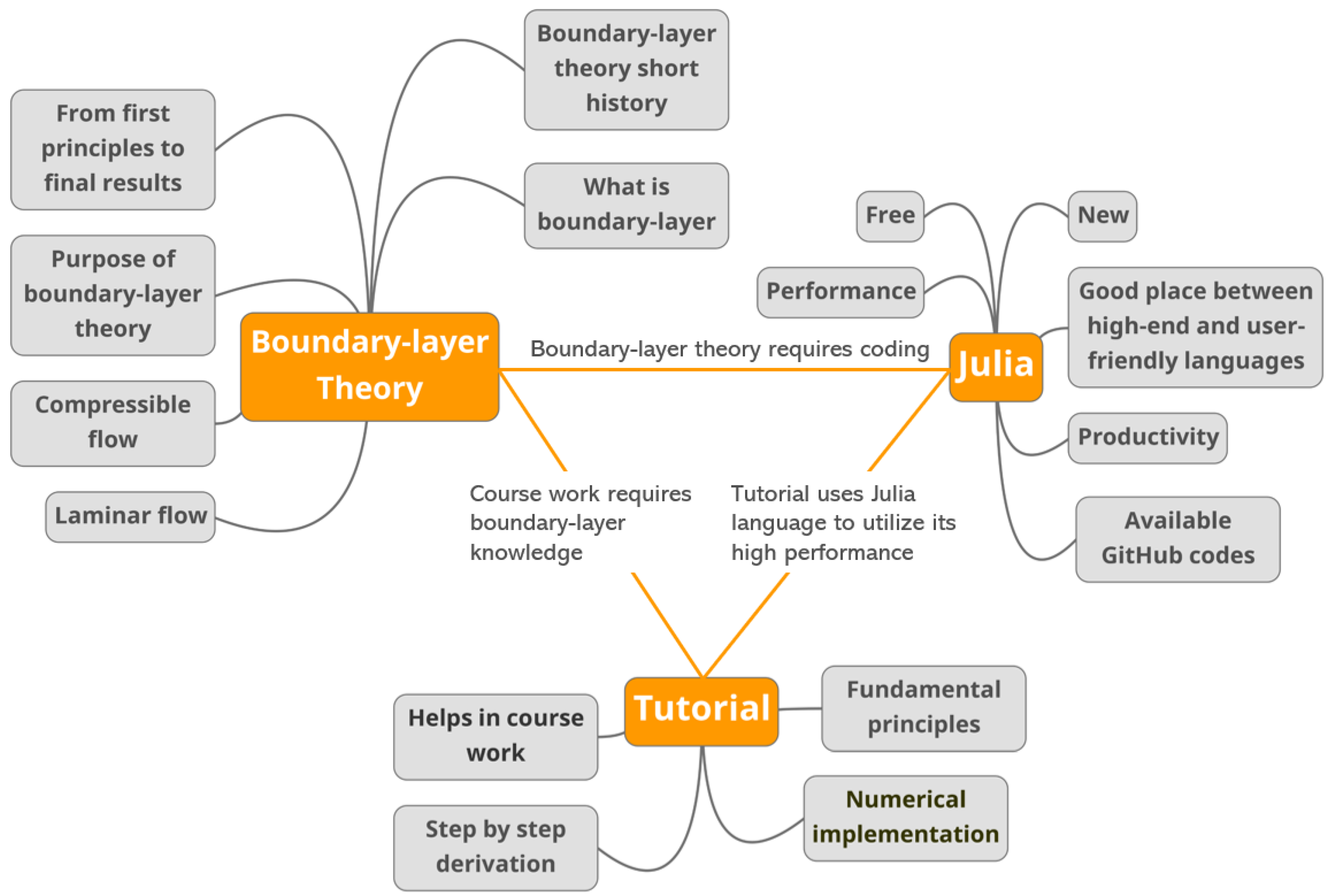
Figure 1.
The visual abstract of the present paper which is mainly designed around 3 major points. Major points are further divided into smaller points which correspond to purposes/ideas of the particular major point. Each major point is connected to one another, which makes them complete.
Figure 1.
The visual abstract of the present paper which is mainly designed around 3 major points. Major points are further divided into smaller points which correspond to purposes/ideas of the particular major point. Each major point is connected to one another, which makes them complete.

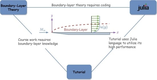
Figure 2.
Schematic description of the flow over a flat plate. The red dashed line corresponds to boundary-layer edge. The boundary-layer velocity profile is illustrated with a blue line. The black dot corresponds to the boundary-layer edge at that station. The density, temperature, and velocity at the boundary-layer edge are and , respectively. The boundary-layer thickness is defined with , which is the function of x.

Figure 3.
The distribution of the (a) velocity and (b) temperature of the compressible Blasius equation obtained by the given code and BL2D boundary-layer solver [20] for freestream Mach number 2.8 and 4.5 where freestream temperatures are 121.11 K and 61.584 K, respectively.
Figure 3.
The distribution of the (a) velocity and (b) temperature of the compressible Blasius equation obtained by the given code and BL2D boundary-layer solver [20] for freestream Mach number 2.8 and 4.5 where freestream temperatures are 121.11 K and 61.584 K, respectively.
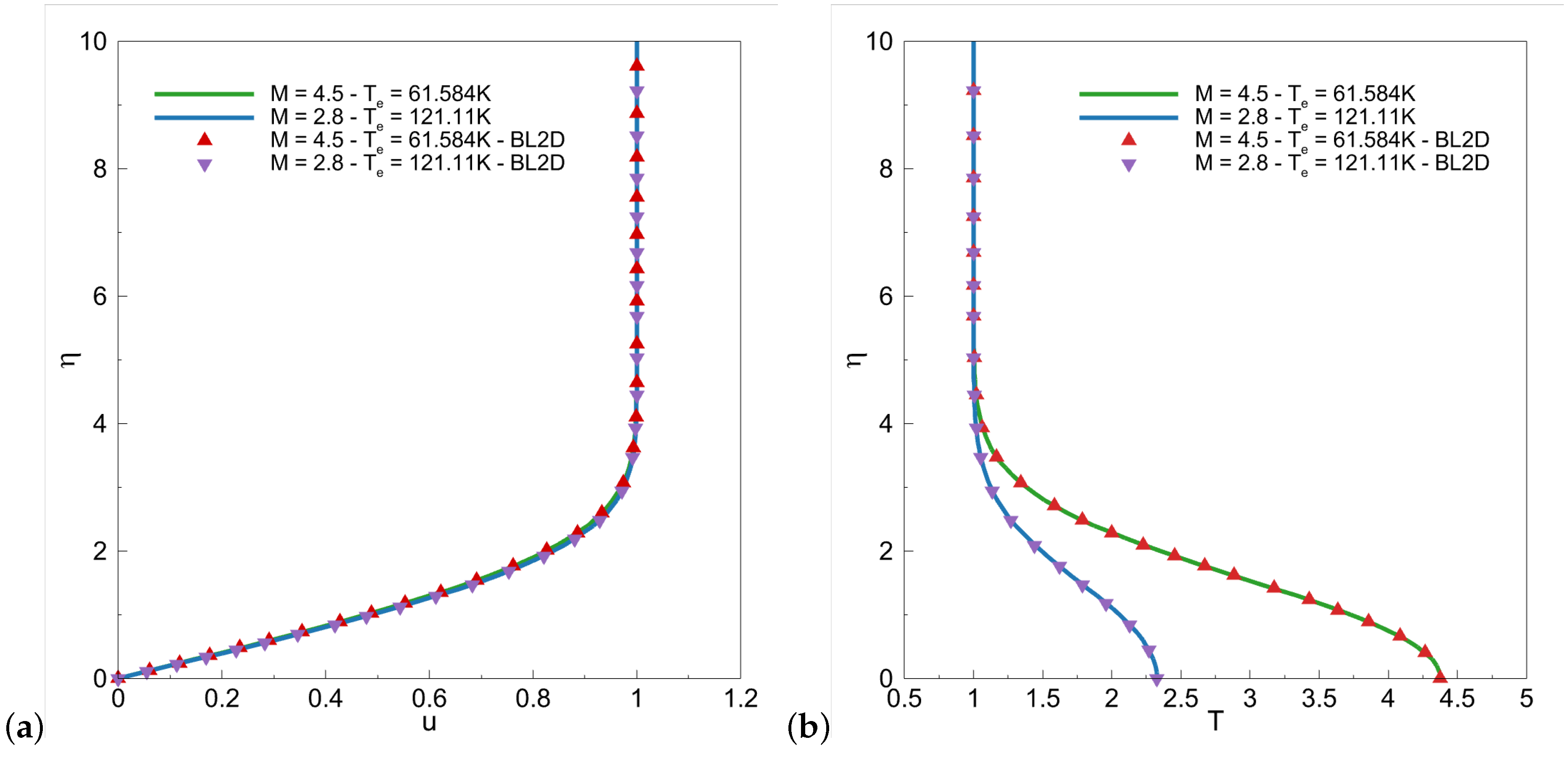
Table 1.
Mean execution times and standard deviations of the Burgers’ equation solver written in MATLAB and Julia by including file operations. The mean execution times are given in second. Ten data points are used in the calculation of the mean and the standard deviation.
Table 1.
Mean execution times and standard deviations of the Burgers’ equation solver written in MATLAB and Julia by including file operations. The mean execution times are given in second. Ten data points are used in the calculation of the mean and the standard deviation.
| File Op. | 10,000 | ||||||
|---|---|---|---|---|---|---|---|
| Included | Julia | MATLAB | Julia | MATLAB | Julia | MATLAB | |
| Loop | Mean | 0.0360 | 0.5214 | 0.1394 | 1.9817 | 0.5592 | 7.8060 |
| STD | 0.0010 | 0.0137 | 0.0017 | 0.0210 | 0.0062 | 0.0522 | |
| Vectorized | Mean | 0.0643 | 0.5145 | 0.2678 | 1.9471 | 1.0042 | 7.7527 |
| STD | 0.0139 | 0.0137 | 0.0287 | 0.0107 | 0.0348 | 0.0402 | |
Table 2.
Mean execution times and standard deviations of the Burgers’ equation solver written in MATLAB and Julia by excluding file operations. The mean execution times are given in second. Ten data points are used in the calculation of the mean and the standard deviation.
Table 2.
Mean execution times and standard deviations of the Burgers’ equation solver written in MATLAB and Julia by excluding file operations. The mean execution times are given in second. Ten data points are used in the calculation of the mean and the standard deviation.
| File Op. | 10,000 | ||||||
|---|---|---|---|---|---|---|---|
| Excluded | Julia | MATLAB | Julia | MATLAB | Julia | MATLAB | |
| Loop | Mean | 0.0059 | 0.0177 | 0.0233 | 0.0651 | 0.0930 | 0.2562 |
| STD | 0.0001 | 0.0031 | 0.0011 | 0.0024 | 0.0005 | 0.0138 | |
| Vectorized | Mean | 0.0437 | 0.0166 | 0.0866 | 0.0564 | 0.4542 | 0.3091 |
| STD | 0.0117 | 0.0021 | 0.0215 | 0.0040 | 0.0584 | 0.0138 | |
Table 3.
Mean execution times and standard deviations of the heat equation solver written in MATLAB and Julia by including file operations. The mean execution times are given in second. Ten data points are used in the calculation of the mean and the standard deviation.
Table 3.
Mean execution times and standard deviations of the heat equation solver written in MATLAB and Julia by including file operations. The mean execution times are given in second. Ten data points are used in the calculation of the mean and the standard deviation.
| File Op. | |||||||
|---|---|---|---|---|---|---|---|
| Included | Julia | MATLAB | Julia | MATLAB | Julia | MATLAB | |
| Loop | Mean | 0.4604 | 3.1921 | 3.3852 | 22.8472 | 25.1985 | 151.5271 |
| STD | 0.0160 | 0.4149 | 0.0132 | 0.4356 | 0.0470 | 0.5615 | |
| Vectorized | Mean | 1.4524 | 3.2964 | 10.0283 | 28.4063 | 81.2305 | 188.5569 |
| STD | 0.1622 | 0.1531 | 0.4356 | 1.0269 | 0.4925 | 0.9425 | |
Table 4.
Mean execution times and standard deviations of the heat equation solver written in MATLAB and Julia by excluding file operations. The mean execution times are given in second. Ten data points are used in the calculation of the mean and the standard deviation.
Table 4.
Mean execution times and standard deviations of the heat equation solver written in MATLAB and Julia by excluding file operations. The mean execution times are given in second. Ten data points are used in the calculation of the mean and the standard deviation.
| File Op. | |||||||
|---|---|---|---|---|---|---|---|
| Excluded | Julia | MATLAB | Julia | MATLAB | Julia | MATLAB | |
| Loop | Mean | 0.1538 | 0.3268 | 1.1964 | 3.7574 | 10.5993 | 28.5775 |
| STD | 0.0038 | 0.0187 | 0.0077 | 0.3274 | 0.1667 | 0.1065 | |
| Vectorized | Mean | 0.8056 | 0.5087 | 8.5873 | 9.3634 | 71.9560 | 67.5810 |
| STD | 0.0706 | 0.0257 | 0.0687 | 0.9880 | 0.4309 | 0.8318 | |
Table 5.
Mean execution times and standard deviations of the compressible Blasius equations solver written in MATLAB and Julia. The mean execution times are given in second. Ten data points are used in the calculation of the mean and the standard deviation.
Table 5.
Mean execution times and standard deviations of the compressible Blasius equations solver written in MATLAB and Julia. The mean execution times are given in second. Ten data points are used in the calculation of the mean and the standard deviation.
| File Op. | 50,000 | 100,000 | 200,000 | ||||
|---|---|---|---|---|---|---|---|
| Excluded | Julia | MATLAB | Julia | MATLAB | Julia | MATLAB | |
| Loop | Mean | 0.0831 | 1.2468 | 0.1631 | 5.1070 | 0.3298 | 39.4378 |
| STD | 0.0054 | 0.0310 | 0.0057 | 0.3006 | 0.0098 | 0.8308 | |
Publisher’s Note: MDPI stays neutral with regard to jurisdictional claims in published maps and institutional affiliations. |
© 2021 by the authors. Licensee MDPI, Basel, Switzerland. This article is an open access article distributed under the terms and conditions of the Creative Commons Attribution (CC BY) license (https://creativecommons.org/licenses/by/4.0/).
Share and Cite
MDPI and ACS Style
Oz, F.; Kara, K. A CFD Tutorial in Julia: Introduction to Compressible Laminar Boundary-Layer Flows. Fluids 2021, 6, 400. https://doi.org/10.3390/fluids6110400
AMA Style
Oz F, Kara K. A CFD Tutorial in Julia: Introduction to Compressible Laminar Boundary-Layer Flows. Fluids. 2021; 6(11):400. https://doi.org/10.3390/fluids6110400
Chicago/Turabian StyleOz, Furkan, and Kursat Kara. 2021. "A CFD Tutorial in Julia: Introduction to Compressible Laminar Boundary-Layer Flows" Fluids 6, no. 11: 400. https://doi.org/10.3390/fluids6110400