
Spin-Up from Rest of a Liquid Metal with Deformable Free Surface in a Cylinder under the Influence of a Uniform Axial Magnetic Field


1
Department of Aeronautics and Astronautics, Tokyo Metropolitan University, Asahigaoka 6-6, Hino 191-0065, Japan
2
School of Mechanical Engineering, Lanzhou Jiaotong University, Lanzhou 730070, China
*
Author to whom correspondence should be addressed.
Fluids 2021, 6(12), 438; https://doi.org/10.3390/fluids6120438
Submission received: 31 October 2021
/
Revised: 25 November 2021
/
Accepted: 29 November 2021
/
Published: 2 December 2021
(This article belongs to the Collection Complex Fluids)
Abstract
:Spin-up from rest of a liquid metal having deformable free surface in the presence of a uniform axial magnetic field is numerically studied. Both liquid and gas phases in a vertically mounted cylinder are assumed to be an incompressible, immiscible, Newtonian fluid. Since the viscous dissipation and the Joule heating are neglected, thermal convection due to buoyancy and thermocapillary effects is not taken into account. The effects of Ekman number and Hartmann number were computed with fixing the Froude number of 1.5, the density ratio of 800, and the viscosity ratio of 50. The evolutions of the free surface, three-component velocity field, and electric current density are portrayed using the level-set method and HSMAC method. When a uniform axial magnetic field is imposed, the azimuthal momentum is transferred from the rotating bottom wall to the core region directly through the Hartmann layer. This is the most striking difference from spin-up of the nonmagnetic case.
1. Introduction
Rotating fluid flows are encountered in a wide variety of industrial occasions, particularly in pumps, water turbines, compressors, wind turbines, and so on. So far, various aspects related to the rotating fluid dynamics have been studied not only for such technical contexts but also for geophysics. Spin-up flow, which is a transient adjustment process of fluid when the rotational speed of the vessel suddenly changes, has been considered as a fundamental topic, and it is still an important problem in rotating fluid dynamics.
The classic and basic case is that an incompressible viscous fluid is completely filled into a cylindrical container, from which the container suddenly begins to rotate around a central axis. In the study by Greenspan and Howard [1] or Wedemeyer [2], a theoretical method was implemented because the complete numerical calculation of the Navier–Stokes equation was difficult at that time due to the underdeveloped computer. Since then, various studies have been carried out to confirm the theory, and numerical elucidation has been attempted since the 1980s [3,4,5]. The important parameter in spin-up is the Ekman number, whose time scale is E−0.5Ω−1 (where E is the Ekman number and Ω is the angular velocity), while the time diffusion scale is E−1Ω−1. This is due to the effect of the meridian flow due to the nonlinear term of the Navier–Stokes equation.
Possible effects on spin-up include fluid compressibility [6], non-axisymmetric case [7], container shape [8], temperature stratification [9,10], and two-phase fluid [11,12,13,14]. Due to these effects, spin-up is affected by the Coriolis force, pressure gradient, and viscous actions, as well as buoyancy and surface tension. Especially in recent years, research on spin-up of liquid metals has emerged in the field of material electromagnetic processing [15,16,17]. In these cases, instead of the rotation of the container itself, a rotating magnetic field is suddenly applied. Although liquid metal is contained in a container, the upper surface is often exposed to contact with gas. In connection with this, Lee et al. [18] studied an MHD flow for the so-called classical spin-up problem in which a cylindrical container abruptly starts to rotate from rest. Their research dealt with the case where the upper part of the cylindrical container had a free surface, assuming application to the Czochralski method [19,20], but did not deal with the deformation of the free surface. However, it was shown that the spin-up time decreases in proportion to the Hartmann number [21] with the increase in magnetic field strength. The timescale is proportional to Ha−1E−1Ω−1 (where Ha is the Hartmann number).
Numerical models are needed to simulate such a free-surface flow in the presence of a magnetic field. Several methods have been reported for numerical studies of free-surface flows based on interface-capturing techniques using fixed mesh systems. For example, the VOF (volume of fluid) and level-set methods are well known to be useful and practical. The difficulty in these methods lies in mass balance during computation, as well as in the accurate estimation of the local mean curvature, especially when the density ratio between the two phases is large. The VOF method [22] is capable of keeping the mass balance, while the level-set method [23] has advantages in accurately estimating the local mean curvature. The CLSVOF (coupled level-set and volume-of-fluid) method [24] combines the advantages of the level-set and VOF methods. Sussman et al. carried out computations of incompressible two-phase flows for the motion of air bubble in water and falling water drops in air using a level-set method [23]. Inamuro et al. succeeded in numerical computation of incompressible two-phase flows with large density differences, such as capillary wave, droplet collision, and bubble flow, using a lattice Boltzmann method [25]. Morley et al. [26] proposed a model of liquid metal free-surface MHD flows for the application of a nuclear fusion reactor. Takatani [27] developed a mathematical model of incompressible MHD flows with free surface and computed several free-surface flows. Tagawa and his group [28,29,30,31,32] carried out the various computations of free-surface flows in the presence of a uniform magnetic field. Lee et al. [18] numerically investigated spin-up from rest of liquid metal in a cylinder under the influence of vertical magnetic field. They successfully computed spin-up even for small Ekman numbers on the order of 10−5 and large Hartmann numbers on the order of 102 with the use of a nonuniform mesh system and Hartmann boundary layer theory. However, they did not take the free-surface deformation into consideration. Therefore, in the present study, the spin-up from rest with free-surface deformation under the influence of a uniform axial magnetic field is numerically investigated using a level-set method.
Section 2 describes mathematical formulations for computing the liquid metal free-surface flow in a rotating cylinder under a uniform magnetic field. In Section 3, we first verify the numerical results by examining a grid dependency test, and then various effects such as surface tension, Ekman number, and Hartmann number on the numerical results are investigated. Section 4 discusses future studies related to the MHD spin-up problem. Section 5 gives the conclusions of this paper.
2. Mathematical Formulations
2.1. Schematic Model for Spin-Up
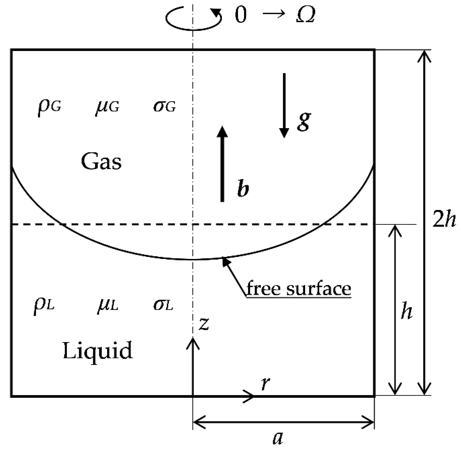
As shown in Figure 1, a liquid metal is partially filled in a vertically mounted cylindrical enclosure with the half depth of the enclosure height, and then the cylinder suddenly starts to rotate around the axis at a constant angular velocity Ω from a stationary condition. The initial height of liquid phase h is the same as the radius of the cylinder a, and the enclosure height is twice the initial liquid height. The fluids themselves also start to rotate due to the shearing force received from the top and bottom plane walls, as well as the sidewall. At the beginning of rotation, the velocity component is limited to only the azimuthal one, but the radial component of velocity is shortly induced by the centrifugal force acting in the vicinity of the plane walls. This secondary flow always occurs irrespective of the single-phase or two-phase case. In the case of two-phase flow, as presented herein, since the lower part of liquid metal is heavier than the upper part of air, the liquid metal tends to accumulate near the sidewall. As sufficient time evolves, the shape of the free surface becomes parabolic since the angular velocity of fluids becomes the same as that of the rotating cylindrical enclosure. However, the transient process of this phenomenon to the final stage has not been well understood because of several factors such as density difference, viscosity difference, and the rotation speed of the cylinder. Moreover, if the uniform magnetic field is applied, the liquid-metal flow is substantially affected by the electromagnetic force, which could be different from the previous understanding of ordinary spin-up from rest with or without the free surface.
2.2. Governing Equations
We assume that the fluid is an incompressible Newtonian fluid for both the liquid and gas phases, and that they are immiscible with each other. In this study, heat source effects such as viscous dissipation and Joule heating are ignored; therefore, an isothermal field within the enclosure is assumed. The induced magnetic field is so small that it can be neglected compared to the intensity of imposed magnetic field due to the smallness of the magnetic Prandtl number. Hence, the governing equations of the continuity of mass, advection equation for density, momentum equations, conservation of electric charge, and Ohm’s law, are respectively expressed below.
It is noted that the density ρ, the viscosity μ and the electric conductivity σ are not constants but depend on whether the local fluid belongs to the liquid or gas phase. We assume that the two-phase fluid flow inside a cylindrical enclosure is axisymmetric. Each term in the momentum equations is considered in the axisymmetric cylindrical coordinate system.
As shown in Figure 1, the direction of gravity is parallel to the axis of the cylindrical enclosure. Hence, the gravity force is simply written as follows:
The viscous force for incompressible fluids can be obtained by taking the divergence of the viscosity stress tensor in the cylindrical coordinate system. The final form for the axisymmetric case becomes
Since the direction of the applied uniform magnetic field is parallel to the axis of cylindrical enclosure and the induced magnetic field is neglected, the electromagnetic force is written as follows:
The continuum surface force (CSF) model [33] is known to be useful for modeling the surface tension acting at the interface. In this study, the gradient of a smoothed step function was employed instead of using the smoothed delta function according to Francois et al. [34]. The surface normal force can be written using the level-set function, which indicates the distance from the liquid–gas interface, as follows:
2.3. Dimensionless Equations
The dimensionless governing equations in the axisymmetric cylindrical coordinate system for analyzing incompressible, immiscible, free-surface flow in the presence of a surface tension and magnetic field are summarized as follows:
The dimensionless variables and nondimensional numbers such as the Ekman, Weber, and Hartmann numbers are defined using the liquid phase properties as follows:
The physical properties such as density, viscosity, and conductivity within the transition region are defined as follows:
Here, Hε(Φ) indicates the smoothed Heaviside step function, and its definition is shown below. In this study, ε was set to 1.5ΔX, which is 1.5 times the width of the grid interval.
In this study, the cylinder aspect ratio was limited to Ar = 1. The initial and boundary conditions were respectively set as follows:
The boundary condition for the level-set function Φ indicates that the contact angle of the liquid was 90°.
2.4. Numerical Methodology
The computational domain was considered within an R–Z cross-section for both the liquid and the gas regions, which were divided into uniform square meshes as shown in Figure 2a. The HSMAC (Highly Simplified Marker and Cell) method [35] was employed to iteratively obtain the pressure and velocity fields. By taking the fluid density into account, i.e., whether each phase is liquid or gas, the simultaneous corrections for the pressure and velocity components were derived as follows:
Here, the subscript i,k indicates the location of computational domain, and the superscript m indicates the step of iteration. The inertial term in the momentum equation is approximated using a third-order upwind scheme called UTOPIA (Uniformly Third-Order Polynomial Algorithm) scheme [36], and the other terms such as viscosity, pressure, and external forces are approximated using the second-order central difference scheme. In the present study, the iterative procedure for the corrections was continued unless the certain threshold for the divergence of velocity (Equation (10)) was satisfied. A similar procedure was employed for the electromagnetic field. The present numerical results, which are shown in the next section, were obtained using in-house codes developed by our laboratory group. Using these codes, which were verified for various fluid flows, we published several studies related to MHD free-surface flows [28,29,30,31,32].
For visualization of the computational results, the Stokes stream function was employed for the meridional velocity and electric current density.
3. Results
3.1. Grid Dependency
Depending on the species of liquid metal, the physical properties such as density, viscosity, and electric conductivity differ extensively. In this study, as a typical case, the density ratio and viscosity ratio were set to 800 and 50, respectively. These two ratios are almost equivalent to a system of water and air. As for the Froude number, Fr = 1.5 was selected because this Froude number allows us to observe a clear free-surface deformation even at an early stage of spin-up, and the liquid phase does not reach the ceiling (top flat wall) even at a well-developed stage.
First of all, the influence of number of meshes for a representative case was examined. Figure 3 shows the free-surface shape for several time instants at the Ekman number with gaseous properties of 0.01 and a Froude number of 1.5 for the three kinds of different mesh system, as indicated in Figure 3. The numbers shown in the vicinity of the sidewall indicate the dimensionless time instants.
At the beginning of rotation, the rate of deformation is rapid near the sidewall, but it becomes less rapid as time evolves. At the time instant 200 (τ = 200), the surface shape is quasi-parabolic, which means that both liquid and gas phases rotate at the same angular velocity, i.e., the state of rigid body rotation is attained. The effect of mesh size seemed not so significant for this case. The deviations among three different meshes are shown at the three time instants of 10, 60 and 200. The grid dependency was quite small between the middle mesh (150 × 300) and the finer mesh (200 × 400). Hereafter, the middle size of mesh system (150 × 300) was employed irrespective of the Ekman number and Hartmann number.
3.2. Effect of Surface Tension
The influence of surface tension on spin-up is examined in this subsection for a case in the absence of a magnetic field. The effect of surface tension is usually dominant in small-scale two-phase flows. Figure 4 shows the numerical results without and with the effect of surface tension for comparison. The two figures look almost the same except near the sidewall. The shape of the free surface is influenced by the surface tension only near the sidewall. This was due to the set of boundary conditions where the contact angle of the level-set function was 90°. In the case of no surface tension, the large value of local curvature at the sidewall was allowed. On the other hand, in the presence of surface tension, the local large value of curvature was not allowed and, therefore, the appearance of surface shape near the sidewall changed as shown in Figure 4b. Hereafter, the surface tension effect was not taken into account for the subsequent results.
3.3. Effect of the Ekman Number
Figure 5 shows the contour lines of azimuthal component of velocity for the four different cases of Ekman number with different time instants. Both liquid and gas phases are visualized, and the range of contour maps is 0 to 1. The red parts were rotating quickly, and the blue parts were at rest. The Froude number was set to 1.5, the density ratio was 800, and the viscosity ratio was 50. With a decrease in the Ekman number, the gradient of azimuthal velocity became large near the liquid–gas interface. This tendency was also observed in the vicinity of the top plain and bottom plain walls, i.e., the boundary layers became thinner with a decrease in the Ekman number. However, the boundary layer thickness was significantly different between the gas boundary layer formed at the top and the liquid boundary layer formed at the bottom since the kinematic viscosity of liquid is 16 times smaller than that of gas. Nevertheless, for small Ekman number cases, the liquid boundary layer became very thin, limiting the numerical accuracy for such cases.
3.4. Spin-Up in the Axial Uniform Magnetic Field
In order to understand the effect of the magnetic field on spin-up, Ha = 50 was chosen in this study. It is understood that the effect of the magnetic field changes depending on the values of other dimensionless parameters. For the current value of the Ekman number, a sufficient magnetic field effect can be expected with Ha = 50. Figure 6 shows a view of electric current density vectors near the free surface at τ = 20. The contour lines with color flood indicate the values of the level-set function (Φ = −0.01. 0.00 and 0.01). The interface width of this analysis was 0.02, since the number of meshes employed in the radial direction was 150. As indicated in Equation (21), in the transitional region of interface, the electric conductivity changes rapidly across the interface; therefore the electric current density in such region should be visualized to verify the computational accuracy for MHD free-surface flows. It is recognized that the electric current density vectors tend to be aligned parallel to the free-surface shape, and those outside of the free surface are zero.
In this paper, the radial and axial components of electric current density were defined at the interface of neighboring staggered meshes, while the azimuthal component was defined at the center of mesh. In the procedure of calculation of the radial and axial components of electric current density, it is necessary to interpolate the electric conductivity at the mesh interfaces since the electric conductivity was defined at the mesh center in this analysis. The interpolated value of electric conductivity at the interfaces was employed in Equation (16) as follows:
This equation denotes a serial connection of resistors, which helps to prevent the electric current density from flowing outside of the gas region.
Figure 7 shows the visualized results at two time instants of τ = 10 and 50 for the velocity field in (a), the electric potential and pressure in (b), and the electric current density field in (c). Only the liquid region is visualized. The upper plots show the time instant of τ = 10 and the lower ones show that of τ = 50. In (a), the left half shows the contour lines of azimuthal velocity, and the right half shows those of meridional circulation (secondary flow) using the Stokes stream function. At the early time stage of τ = 10, the azimuthal velocity is not well propagated into the core region; therefore, the surface shape in the core seems rather flat. At the nearly final stage of the spin-up process (τ = 50), the free-surface shape seems to be parabolic and the strength of the secondary flow is much weaker than that of the early stage of τ = 10, as indicated in the range of the contour legend. As shown in (b), the electric potential profile depended mostly on the radius. It took its maximum at the sidewall and its minimum at the center axis. The pressure profile indicates that its contour lines were parallel near the free surface, and the maximum pressure point was located at the bottom corner. In (c), the meridional electric current density is shown in the right half and the azimuthal current density is shown in the left half. The meridional current circulated in the contour-clockwise direction, and then the radially outward current near the bottom walls reduced the azimuthal flow. On the other hand, the azimuthal current density was mostly confined within the boundary layer formed in the vicinity of the bottom wall. As shown in Equation (16), this azimuthal current density was the same as the radial component of fluid velocity. Due to the Lorentz force acting at the boundary layer, its thickness decreased as the Hartmann number increased.
Figure 8 shows a comparison of the velocity field without and with the axial magnetic field. The left-hand figures are the cases without the magnetic field, while the right-hand ones are those with the magnetic field. As a represented case, Ha = 50 was examined. It should be noted that the range of contour maps is not common since the secondary flow attenuates as time evolves. On the other hand, the contour of azimuthal velocity always ranged from 0 to 1 for all the time instants. When no magnetic field was applied, the spin-up of gas was much faster than that of liquid because of the difference in the kinematic viscosity. Hence, the liquid experienced azimuthal momentum from not only the rotating bottom wall but also the faster gas flow, as recognized in (Figure 8e). Nevertheless, there was still a stagnant region in the core region. When a uniform axial magnetic field was applied, the boundary layer formed in the vicinity of the rotating bottom wall was thinner than that of the nonmagnetic case. The most striking difference from the nonmagnetic case was that the azimuthal velocity took place in the core region even at the early stage because the azimuthal momentum was transferred from the rotating bottom wall to the core region directly through the Hartmann layer. As a result, it can be recognized that the free surface far from the sidewall began to deform immediately after the start of the rotation. This tendency would become more pronounced as the Hartmann number is increased. However, since it is known that several grids are required within the Hartmann layer to keep its numerical accuracy, the computation of such a high Hartmann number would be more difficult. To overcome this difficulty without having several grids in the layer, a special treatment of the Hartmann layer [18] could be useful even in this deformable free-surface problem.
4. Discussion
In this study, a numerical model for solving the free-surface spin-up flow of a liquid metal placed in a cylindrical container was shown under the imposition of a uniform axial magnetic field. As a result of neglecting viscous dissipation and Joule heat generation, the assumption of axial symmetry with respect to the isothermal flow field was made. As shown by the computational results, a smaller Ekman number required a finer grid resolution and a longer calculation time. Therefore, we did not mention the results of several Ekman numbers (especially with small Ekman numbers) in this paper. In addition, since there is a meridional flow in the flow field, it is quite natural that the axisymmetric flow field becomes three-dimensional due to centrifugal force instability when the Ekman number becomes smaller. By conducting a three-dimensional simulation, it is possible to pay attention to such a transition of the flow field, which is one of the future issues to be examined in the MHD spin-up problem.
5. Conclusions
Numerical computations of spin-up from rest of a liquid metal with a deformable free surface were carried out under the influence of a uniform axial magnetic field. The evolutions of three components of velocity and electric current density were successfully obtained using the level-set method and HSMAC method. The flow phenomenon with a free surface under the magnetic field depends on various dimensionless numbers and the geometry of the container. Since it is not possible to investigate all the effects of dimensionless parameters in detail, the effects of Weber number, Ekman number, and Hartmann number were computed with a density ratio of 800, viscosity ratio of 50, Ar = 1, and Fr = 1.5.
During spin-up in the absence of a magnetic field, it was found that the development rate of the azimuthal velocity of the gas phase was much faster than that of the liquid phase due to the difference in the physical properties of the liquid and the gas. This was because the Ekman number based on the liquid property was 6.25 × 10⁻⁴, while the Ekman number of the gas was 0.01, i.e., 16 times larger when the rotation speed of the container was fixed. Due to this difference in the azimuthal velocity between the gas and the liquid, the liquid received azimuthal momentum from that of air flow. Although such a characteristic phenomenon as a two-phase flow was observed, there was no significant difference from the single-phase spin-up in the development process of the meridional flow.
On the other hand, during spin-up when the magnetic field was applied, the transfer mechanism of the azimuthal momentum was fundamentally different from that without a magnetic field due to the influence of the Lorentz force acting only on the liquid phase. It was found that the azimuthal momentum was directly transferred in the axial direction from the rotating bottom wall to the core through the Hartmann layer. Since the azimuthal velocity began to develop from the initial stage of spin-up, the deformation of the free surface also began accordingly. This was the most notable difference from the nonmagnetic spin-up case.
Author Contributions
Conceptualization, T.T. and K.S.; methodology, T.T.; software, T.T. and K.S.; validation, T.T.; formal analysis, T.T.; investigation, T.T.; resources, T.T. and K.S.; data curation, T.T.; writing—original draft preparation, T.T.; writing—review and editing, K.S.; visualization, T.T.; supervision, T.T.; project administration, T.T.; funding acquisition, T.T. and K.S. All authors have read and agreed to the published version of the manuscript.
Funding
This research received no external funding.
Institutional Review Board Statement
Not applicable.
Informed Consent Statement
Not applicable.
Data Availability Statement
The data presented in this study are available on request from the corresponding author.
Conflicts of Interest
The authors declare no conflict of interest.
Nomenclature
| a | radius of cylindrical enclosure (m) |
| Ar | aspect ratio = a/h (-) |
| b0 | absolute value of magnetic flux density (T) |
| b | magnetic flux density (T) |
| E | Ekman number (-) |
| eR | unit vector in radial direction (-) |
| eZ | unit vector in axial direction (-) |
| eθ | unit vector in azimuthal direction (-) |
| fst | surface normal force (N/m3) |
| Fr | Froude number (-) |
| g | gravitational acceleration (m/s2) |
| g | absolute value of gravitational acceleration (m/s2) |
| h | initial height of liquid (m) |
| Ha | Hartmann number (-) |
| Hε(φ) | smoothed Heaviside step function (-) |
| j | electric current density = (jr, jθ, jz) (A/m2) |
| jr | radial component of electric current density (A/m2) |
| jz | axial component of electric current density (A/m2) |
| jθ | azimuthal component of electric current density (A/m2) |
| J | dimensionless electric current density (-) |
| JR | dimensionless radial component of electric current density (-) |
| JZ | dimensionless axial component of electric current density (-) |
| Jθ | dimensionless azimuthal component of electric current density (-) |
| p | pressure (Pa) |
| P | dimensionless pressure (-) |
| r | radial coordinate (m) |
| R | dimensionless r coordinate (-) |
| t | time (s) |
| u | velocity = (u, v, w) (m/s) |
| u | radial velocity component (m/s) |
| U | dimensionless radial velocity component (-) |
| v | azimuthal velocity component (m/s) |
| V | dimensionless azimuthal velocity component (-) |
| w | axial velocity component (m/s) |
| W | dimensionless axial velocity component (-) |
| We | Weber number (-) |
| z | axial coordinate (m) |
| Z | dimensionless z-coordinate (-) |
| Greek symbols | |
| γ | surface tension (N/m) |
| δε(φ) | smoothed Dirac delta function (1/m) |
| κ | curvature of interface (1/m) |
| μ | viscosity (Pa·s) |
| ν | kinematic viscosity = μ/ρ (m2/s) |
| ρ | density (kg/m3) |
| σ | electric conductivity (1/(Ω·m)) |
| τ | dimensionless time (-) |
| φ | level-set function (m) |
| Φ | dimensionless level-set function (-) |
| ψe | electric potential (V) |
| Ψe | dimensionless electric potential (-) |
| ΨJ | Stokes stream function for electric current density (-) |
| ΨS | Stokes stream function for velocity (-) |
| Ω | angular velocity (rad/s) |
| Subscripts or superscripts | |
| G | gas |
| i,k | grid point |
| L | liquid |
| n | time step |
| m | iteration number |
| Φ | dependence of level-set function |
References
- Greenspan, H.P.; Howard, L.N. On a time-dependent motion of a rotating fluid. J. Fluid Mech. 1963, 17, 385–404. [Google Scholar] [CrossRef]
- Wedemeyer, E.H. The unsteady flow within a spinning cylinder. J. Fluid Mech. 1964, 20, 383–399. [Google Scholar] [CrossRef] [Green Version]
- Watkins, W.B.; Hussey, R.G. Spin-up from rest in a cylinder. Phys. Fluids 1977, 20, 1596–1604. [Google Scholar] [CrossRef]
- Hyun, J.M.; Leslie, F.; Fowlis, W.W.; Warn-Varnas, A. Numerical solutions for spin-up from rest in a cylinder. J. Fluid Mech. 1983, 127, 263–281. [Google Scholar] [CrossRef]
- Park, J.S.; Hyun, J.M. Review on open-problems of spin-up flow of an incompressible fluid. J. Mech. Sci. Technol. 2008, 22, 780. [Google Scholar] [CrossRef]
- Hyun, J.M.; Park, J.S. Spin-up from rest of a compressible fluid in a rapidly rotating cylinder. J. Fluid Mech. 1992, 237, 413–434. [Google Scholar] [CrossRef]
- Henderson, D.M.; Lopez, J.M.; Stewart, D.L. Vortex evolution in non-axisymmetric impulsive spin-up from rest. J. Fluid Mech. 1996, 324, 109–134. [Google Scholar] [CrossRef]
- Van de Konijnenberg, J.A.; Van Heijst, G.J.F. Free-surface effects on spin-up in a rectangular tank. J. Fluid Mech. 1997, 334, 189–210. [Google Scholar] [CrossRef]
- Hyun, J.M. Axisymmetric flows in spin-up from rest of a stratified fluid in a cylinder. Geophys. Astrophys. Fluid Dyn. 1983, 23, 127–141. [Google Scholar] [CrossRef]
- Duck, P.; Foster, M. Spin-up of homogeneous and stratified fluids. Annu. Rev. Fluid Mech. 2001, 33, 231–263. [Google Scholar] [CrossRef] [Green Version]
- Homicz, G.F.; Gerber, N. Numerical model for fluid spin-up from rest in a partially filled cylinder. J. Fluids Eng. 1987, 109, 194–197. [Google Scholar] [CrossRef]
- Choi, S.; Kim, J.W.; Hyun, J.M. Experimental investigation of the flow with a free surface in an impulsively rotating cylinder. J. Fluids Eng. 1991, 113, 245–249. [Google Scholar] [CrossRef]
- Maas, L.R.M. Nonlinear and free-surface effects on the spin-down of barotropic axisymmetric vortices. J. Fluid Mech. 1993, 246, 117–141. [Google Scholar] [CrossRef]
- Kim, K.Y.; Hyun, J.M. Spin-up from rest of a two-layer liquid in a cylinder. J. Fluids Eng. 1994, 116, 808–814. [Google Scholar] [CrossRef]
- Nikrityuk, P.A.; Ungarish, M.; Eckert, K.; Grundmann, R. Spin-up of a liquid metal flow driven by a rotating magnetic field in a finite cylinder: A numerical and an analytical study. Phys. Fluids 2005, 17, 067101. [Google Scholar] [CrossRef]
- Nikrityuk, P.A.; Eckert, S.; Eckert, K. Spin-up and spin-down dynamics of a liquid metal driven by a single rotating magnetic field pulse. Eur. J. Mech. B/Fluids 2008, 27, 177–201. [Google Scholar] [CrossRef]
- Vogt, T.; Grants, I.; Eckert, S.; Gerbeth, G. Spin-up of a magnetically driven tornado-like vortex. J. Fluid Mech. 2013, 736, 641–662. [Google Scholar] [CrossRef]
- Lee, C.H.; Tagawa, T.; Ozoe, H.; Hyun, J.M. Spin-up from rest in a cylinder of an electrically conducting fluid in an axial magnetic field. Acta Mech. 2006, 186, 203–220. [Google Scholar] [CrossRef]
- Galazka, Z. Czochralski method. In Gallium Oxide: Materials Properties, Crystal Growth, and Devices; Higashiwaki, M., Fujita, S., Eds.; Springer: Cham, Switzerland, 2020; Volume 293, pp. 15–36. [Google Scholar]
- Ozoe, H.; Szmyd, J.S.; Tagawa, T. Magnetic fields in semiconductor crystal growth. In Magnetohydrodynamics; Molokov, S., Moreau, R., Moffatt, K., Eds.; Springer: Dordrecht, The Netherlands, 2007; pp. 375–390. [Google Scholar]
- Moreau, R.; Molokov, S. Julius Hartmann and his followers: A review on the properties of the Hartmann layer. In Magnetohydrodynamics; Molokov, S., Moreau, R., Moffatt, K., Eds.; Springer: Dordrecht, The Netherlands, 2007; pp. 155–170. [Google Scholar]
- Scardovelli, R.; Zaleski, S. Direct numerical simulation of free-surface and interfacial flow. Annu. Rev. Fluid Mech. 1999, 31, 567–603. [Google Scholar] [CrossRef] [Green Version]
- Sussman, M.; Smereka, P.; Osher, S. A level set approach for computing solutions to incompressible two-phase flow. J. Comput. Phys. 1994, 114, 146–159. [Google Scholar] [CrossRef]
- Sussman, M.; Puckett, E.G. A coupled level set and volume-of-fluid method for computing 3D and axisymmetric incompressible two-phase flows. J. Comput. Phys. 2000, 162, 301–337. [Google Scholar] [CrossRef] [Green Version]
- Inamuro, T.; Ogata, T.; Tajima, S.; Konishi, N. A lattice Boltzmann method for incompressible two-phase flows with large density differences. J. Comput. Phys. 2004, 198, 628–644. [Google Scholar] [CrossRef]
- Morley, N.; Smolentsev, S.; Munipalli, R.; Ni, M.-J.; Gao, D.; Abdou, M. Progress on the modeling of liquid metal, free surface, MHD flows for fusion liquid walls. Fusion Eng. Des. 2004, 72, 3–34. [Google Scholar] [CrossRef]
- Takatani, K. Mathematical modeling of incompressible MHD flows with free surface. ISIJ Int. 2007, 47, 545–551. [Google Scholar] [CrossRef] [Green Version]
- Tagawa, T. Numerical simulation of a falling droplet of liquid metal into a liquid layer in the presence of a uniform vertical magnetic field. ISIJ Int. 2005, 45, 954–961. [Google Scholar] [CrossRef] [Green Version]
- Tagawa, T. Numerical simulation of two-phase flows in the presence of a magnetic field. Math. Comput. Simul. 2006, 72, 212–219. [Google Scholar] [CrossRef]
- Tagawa, T. Numerical simulation of liquid metal free-surface flows in the presence of a uniform static magnetic field. ISIJ Int. 2007, 47, 574–581. [Google Scholar] [CrossRef] [Green Version]
- Tagawa, T.; Ozoe, H. Effect of external magnetic fields on various free-surface flows. Prog. Comput. Fluid Dyn. Int. J. 2008, 8, 461–468. [Google Scholar] [CrossRef]
- Shibasaki, Y.; Ueno, K.; Tagawa, T. Computation of a rising bubble in an enclosure filled with liquid metal under vertical magnetic fields. ISIJ Int. 2010, 50, 363–370. [Google Scholar] [CrossRef]
- Brackbill, J.U.; Kothe, D.B.; Zemach, C. A continuum method for modeling surface tension. J. Comput. Phys. 1992, 100, 335–354. [Google Scholar] [CrossRef]
- Francois, M.; Cummins, S.J.; Dendy, E.D.; Kothe, D.B.; Sicilian, J.M.; Williams, M.W. A balanced-force algorithm for continuous and sharp interfacial surface tension models within a volume tracking framework. J. Comput. Phys. 2006, 213, 141–173. [Google Scholar] [CrossRef]
- Hirt, C.; Nichols, B.; Romero, N. A Numerical Solution Algorithm for Transient Fluid Flows; Los Alamos Scientific Laboratory Report: Santa Fe, NM, USA, 1975. [Google Scholar]
- Tagawa, T.; Ozoe, H. Effect of Prandtl number and computational schemes on the oscillatory natural convection in an enclosure. Numer. Heat Transf. Part A Appl. 1996, 30, 271–282. [Google Scholar] [CrossRef]
Figure 1.
Flow geometry and coordinates in the meridional plane. The initial condition for the gas–liquid interface is shown with the broken line, while the interface after sudden rotation at a time instant is shown with the solid line. A uniform axial magnetic field is applied.
Figure 1.
Flow geometry and coordinates in the meridional plane. The initial condition for the gas–liquid interface is shown with the broken line, while the interface after sudden rotation at a time instant is shown with the solid line. A uniform axial magnetic field is applied.

Figure 2.
The staggered mesh system employed in the axisymmetric cylindrical coordinate system. The pressure (P), the azimuthal component of velocity (V), and the meridional components of velocity (U, W) are depicted in (a), whereas the electric potential (Ψe), the azimuthal component of current density (Jθ), and the meridional components of current density (JR, JZ) are depicted in (b). The physical properties such as density, viscosity, and electric conductivity are defined at the mesh center. Those values at the mesh interface are interpolated. (a) Fluid flow field; (b) Electromagnetic field.
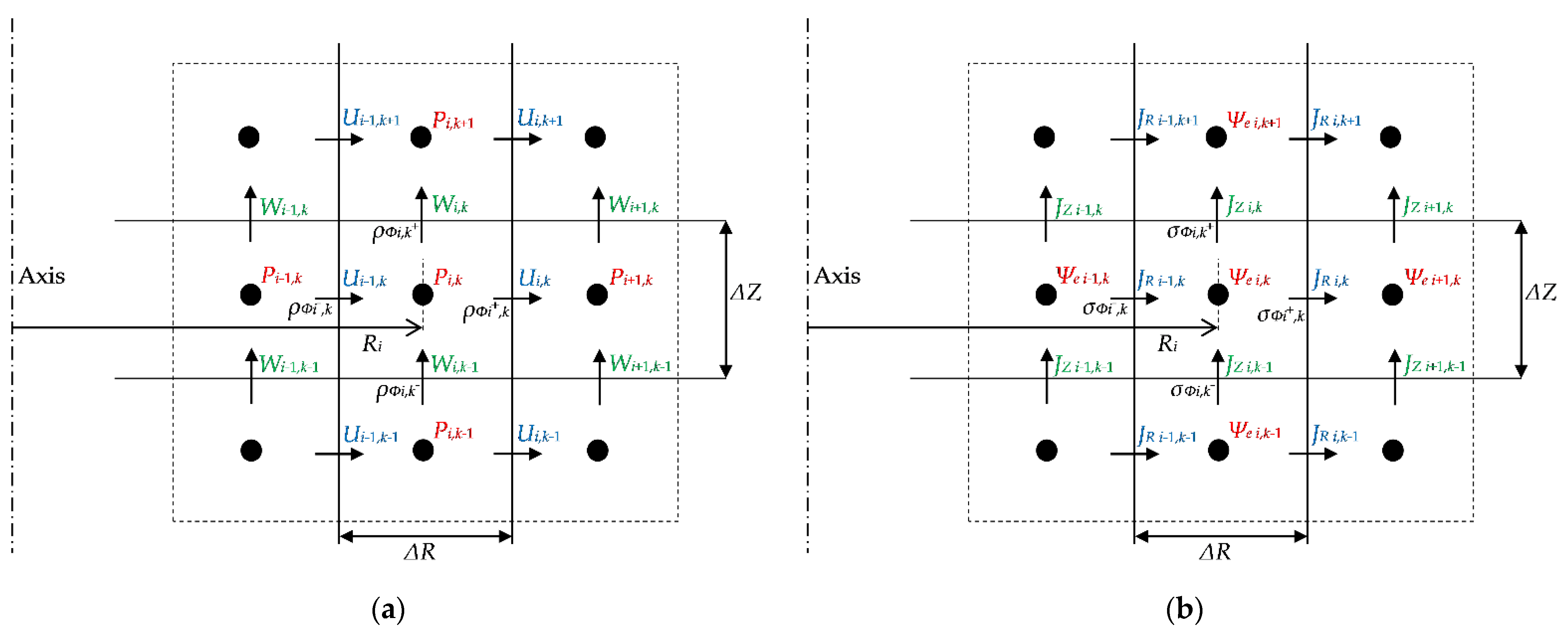
Figure 3.
Dependency of grid size on free-surface shape near the sidewall at the three time instants of τ = 10, 60, and 200 for Ar = 1, E = 6.25 × 10⁻⁴, Fr = 1.5, and Ha = 0. The blue color indicates the case of the coarse grid (100 × 200), the green color is that of the baseline grid (150 × 300), and the red color is the fine grid (200 × 400).
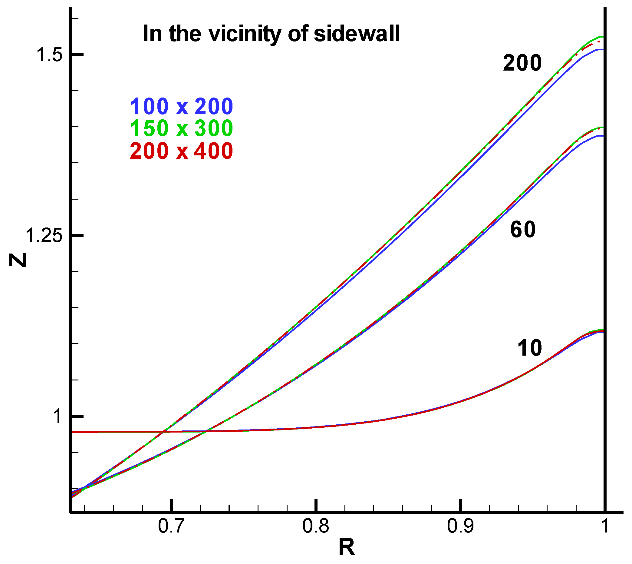
Figure 4.
Effect of surface tension on free-surface shape for Ar = 1, E = 6.25 × 10⁻⁴, Fr = 1.5, and Ha = 0 at τ = 60. The left half shows the contour of the azimuthal velocity (V) and the right half shows the Stokes stream function (ΨS). (a) Without surface tension (We → ∞); (b) with surface tension (We = 800).
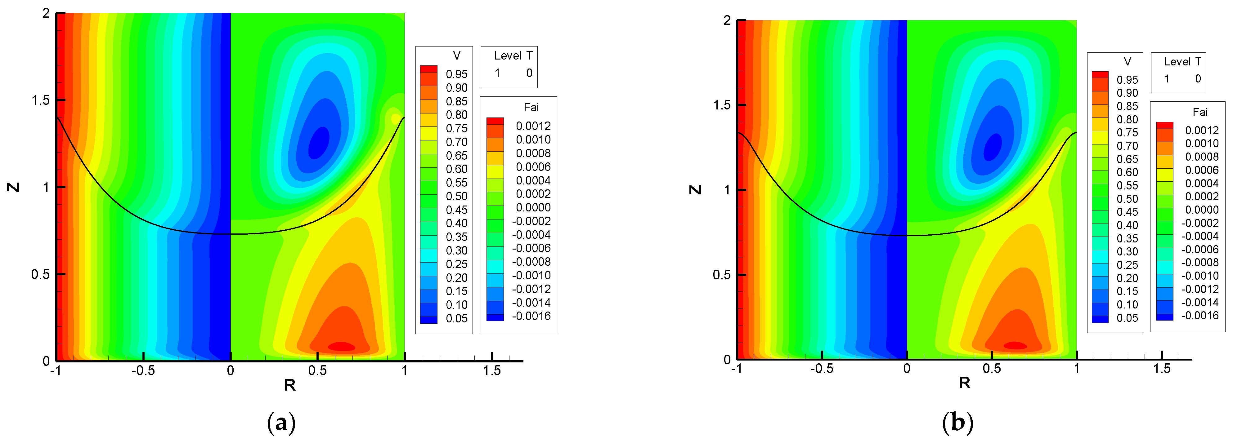
Figure 5.
Effect of the Ekman number on the azimuthal component of velocity without surface tension for Ar = 1, Fr = 1.5, and Ha = 0. (a) E = 6.25 × 10⁻⁴, τ = 25; (b) E = 1.875 × 10⁻⁴, τ = 50; (c) E = 6.25 × 10⁻⁵, τ = 100; (d) E = 1.875 × 10⁻⁵, τ = 200.
Figure 5.
Effect of the Ekman number on the azimuthal component of velocity without surface tension for Ar = 1, Fr = 1.5, and Ha = 0. (a) E = 6.25 × 10⁻⁴, τ = 25; (b) E = 1.875 × 10⁻⁴, τ = 50; (c) E = 6.25 × 10⁻⁵, τ = 100; (d) E = 1.875 × 10⁻⁵, τ = 200.
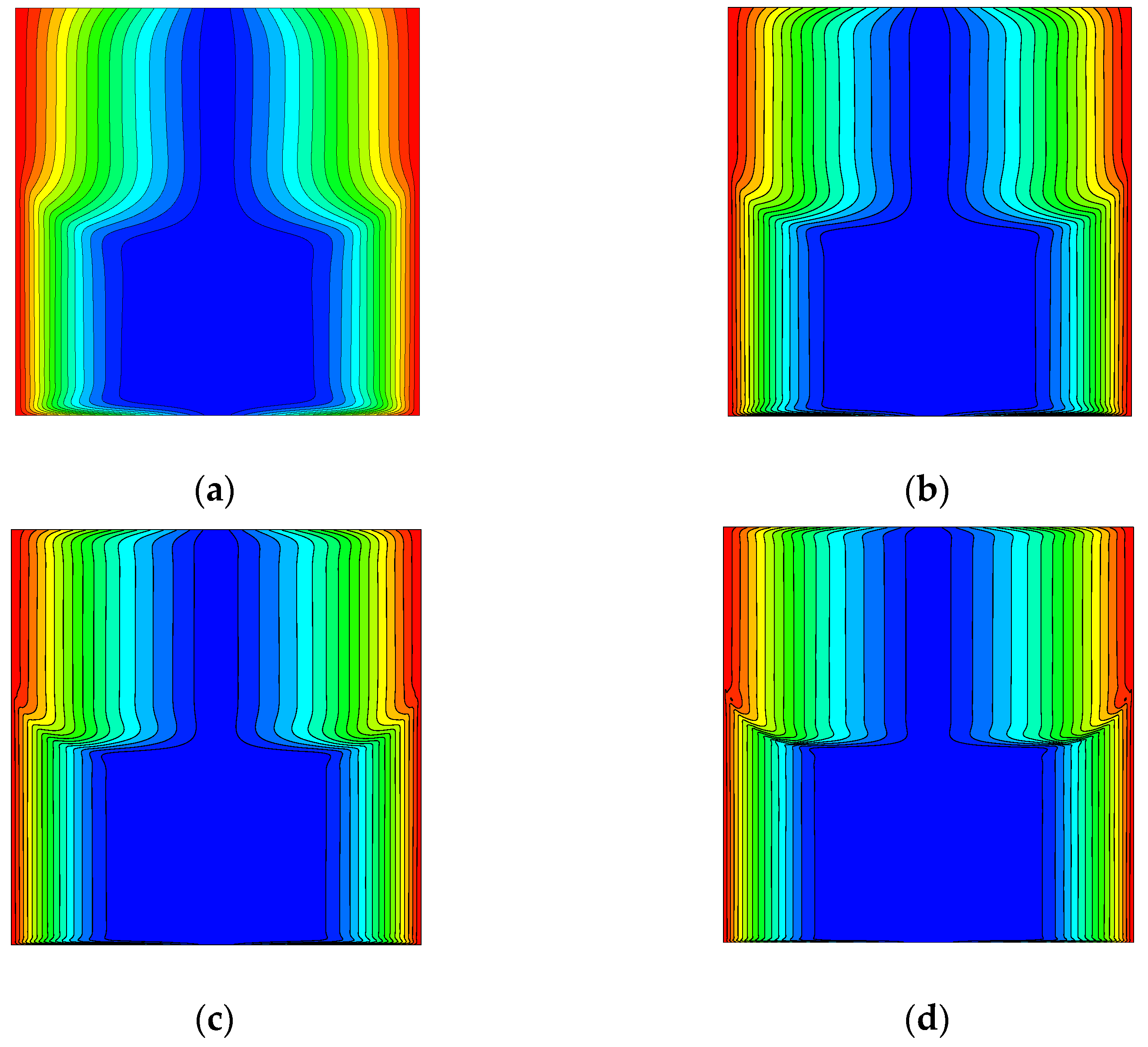
Figure 6.
Meridional electric current density vectors with contour lines of level-set function in the vicinity of the sidewall for Ar = 1, E = 6.25 × 10⁻⁴, Fr = 1.5 and Ha = 50 at τ = 20. The blue part is liquid (conducting fluid) while the white part is gas (nonconducting fluid). The diffused interface is indicated by the green and pink colors.
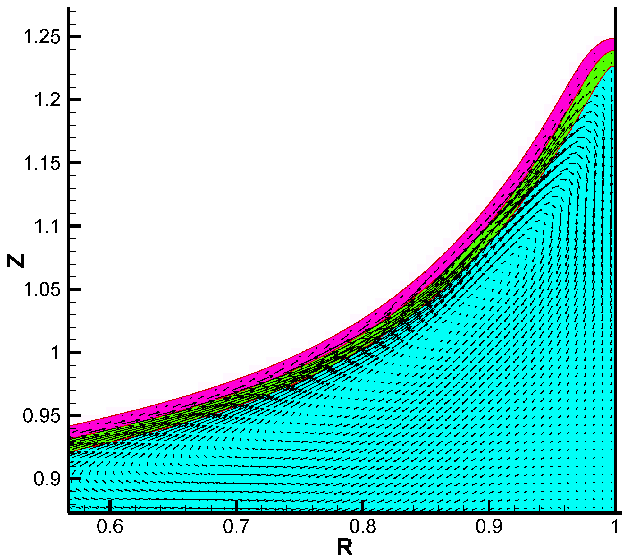
Figure 7.
Spin-up in the presence of magnetic field with free surface for Ar = 1, E = 6.25 × 10⁻⁴, Fr = 1.5 and Ha = 50 at τ = 10 (upper plots) and 50 (lower plots). (a) The left half is the contour map of azimuthal velocity, and the right half is the Stokes stream function; (b) the left half is the contour map of electric potential, and the right half is the pressure; (c) the left half is the contour map of azimuthal current density, and the right half is the meridional current density. It should be noted that the range of contour maps is not common since the secondary flow attenuates as time evolves. (a) Azimuthal velocity (V) and Stokes stream function (ΨS); (b) Electric potential (Ψe) and Pressure (P); (c) Azimuthal current density (Jθ) and Meridional current density (ΨJ).
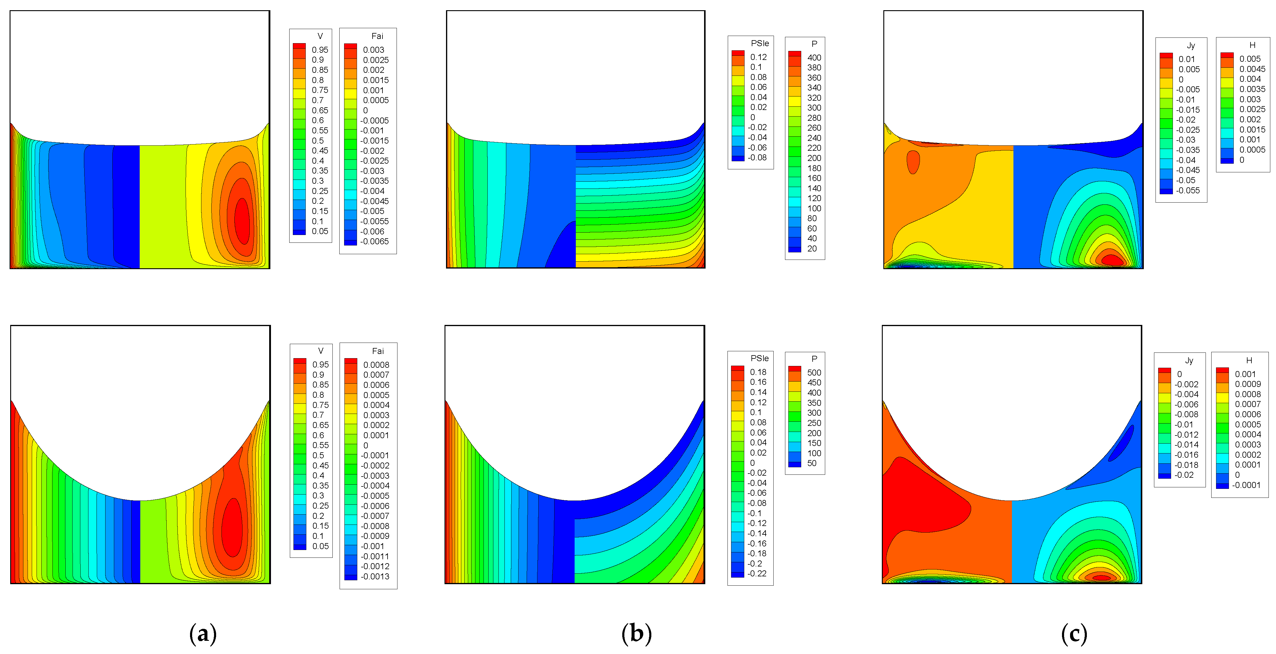
Figure 8.
Contour maps of azimuthal velocity shown on the left and meridional flow (Stokes stream function) shown on the right with free-surface evolution for Ar = 1, E = 6.25 × 10⁻⁴, and Fr = 1.5 at τ = 5 in (a,b), 10 in (c,d), and 20 in (e,f). The left-hand plots show the case of Ha = 0, and the right-hand plots show the case of Ha = 50. (a) τ = 5, Ha = 0; (b) τ = 5, Ha = 50; (c) τ = 10, Ha = 0; (d) τ = 10, Ha = 50; (e) τ = 20, Ha = 0; (f) τ = 20, Ha = 50.

Publisher’s Note: MDPI stays neutral with regard to jurisdictional claims in published maps and institutional affiliations. |
© 2021 by the authors. Licensee MDPI, Basel, Switzerland. This article is an open access article distributed under the terms and conditions of the Creative Commons Attribution (CC BY) license (https://creativecommons.org/licenses/by/4.0/).
Share and Cite
MDPI and ACS Style
Tagawa, T.; Song, K. Spin-Up from Rest of a Liquid Metal with Deformable Free Surface in a Cylinder under the Influence of a Uniform Axial Magnetic Field. Fluids 2021, 6, 438. https://doi.org/10.3390/fluids6120438
AMA Style
Tagawa T, Song K. Spin-Up from Rest of a Liquid Metal with Deformable Free Surface in a Cylinder under the Influence of a Uniform Axial Magnetic Field. Fluids. 2021; 6(12):438. https://doi.org/10.3390/fluids6120438
Chicago/Turabian StyleTagawa, Toshio, and Kewei Song. 2021. "Spin-Up from Rest of a Liquid Metal with Deformable Free Surface in a Cylinder under the Influence of a Uniform Axial Magnetic Field" Fluids 6, no. 12: 438. https://doi.org/10.3390/fluids6120438