Lagrangian vs. Eulerian: An Analysis of Two Solution Methods for Free-Surface Flows and Fluid Solid Interaction Problems

Abstract

As a step towards addressing a scarcity of references on this topic, we compared the Eulerian and Lagrangian Computational Fluid Dynamics (CFD) approaches for the solution of free-surface and Fluid–Solid Interaction (FSI) problems. The Eulerian approach uses the Finite Element Method (FEM) to spatially discretize the Navier–Stokes equations. The free surface is handled via the volume-of-fluid (VOF) and the level-set (LS) equations; an Immersed Boundary Method (IBM) in conjunction with the Nitsche’s technique were applied to resolve the fluid–solid coupling. For the Lagrangian approach, the smoothed particle hydrodynamics (SPH) method is the meshless discretization technique of choice; no additional equations are needed to handle free-surface or FSI coupling. We compared the two approaches for a flow around cylinder. The dam break test was used to gauge the performance for free-surface flows. Lastly, the two approaches were compared on two FSI problems—one with a floating rigid body dropped into the fluid and one with an elastic gate interacting with the flow. We conclude with a discussion of the robustness, ease of model setup, and versatility of the two approaches. The Eulerian and Lagrangian solvers used in this study are open-source and available in the public domain.

1. Introduction

Insofar as the space discretization step is concerned, the majority of CFD models can be classified as: (i) Eulerian approaches, where the unknown state variables are attached to stationary observers; or (ii) Lagrangian approaches, in which the unknown state variables are attached to moving observers. The two approaches are vastly different, and this contribution’s goal was to shed light onto how they compare when used in conjunction with 3D applications that involve interactions with the solid phase.

Eulerian methods have been successfully applied and are very popular in CFD. Indeed, Finite Difference (FD) represents a robust technique for solving partial differential equations on simple domains, while the Finite Volume (FV) has been predominantly applied in fluid flows with complex geometries. Conversely, the Lagrangian methods gained traction only about two decades ago, although the idea of using Lagrangian discretization dates back to 1957 [1]. Among Lagrangian methods, SPH [2,3] has been widely adopted as the low-order approximation of choice for a variety of problems [4], while Moving Least Squares and Radial Basis Functions emerged as the leading high-order meshless methods [5,6,7,8].

For the class of free-surface flows, Eulerian approaches rely on either interface-tracking or interface-capturing techniques. The former is considered more accurate; yet, it involves an update stage in the computational mesh as the shape of the spatial domain occupied by the fluid changes in time. The latter is more flexible in terms of meshing, since the solution relies on one fixed spatial grid that contains two fluid phases. Owing to the introduction of two distinct phases, interface-capturing methods require the solution of additional equations governing the advection of the interface and/or conservation of the phase fraction [9,10,11,12]. The ability to handle two distinct phases is critical in many practical applications in which two or more fluids with different viscosities and densities play equally important roles in the problem, e.g., in the oil and gas industries. On the other hand, handling free-surface problems is more straightforward in Lagrangian approaches. Owing to their meshless nature, these methods eschew the costly re-meshing requirement of interface-tracking methods.

For FSI problems, just as for free-surface flows, the Eulerian approaches are challenged by large mesh deformations, which call upon remeshing operations. A widely used approach is the Arbitrary Lagrangian–Eulerian (ALE) method [13], which handles well sufficiently small mesh deformation, yet it becomes expensive when the motion of the solid objects is relatively large. The IBM [14] addresses this shortcoming by implicitly treating the solid objects, as opposed to the ALE explicit representation of solid bodies that calls for body-fitted meshing. Thus, IBM alleviates the mesh deformation conundrum at the cost of a higher mesh resolution in the vicinity of the solid objects.

Handling FSI problems with complex geometries comes more naturally to meshless methods, e.g., SPH, owing to the their Lagrangian nature that interfaces well with the Lagrangian framework used in solid mechanics [15]. However, SPH-based methods generally have enjoyed a somewhat limited adoption due to their reduced order and deficiencies in numerical approximation near boundaries [5]. Kernel-correction methods have been recently proposed to enforce linear consistency and second-order accuracy, yet they alter the conservation properties of SPH [16,17,18,19,20]. Likewise, the use of larger support basis functions improves robustness but leads to a higher computational cost.

Against this backdrop, this contribution sought to provide insight into a simple question of practical interest: how do the Lagrangian and Eulerian approaches compare when used in non-trivial problems? A pen-and-paper attempt to settle this question is unlikely to be fruitful for nontrivial 3D problems. Indeed, these approaches are too complex in their formulation and depend on too many factors in their software implementation for a pen-and-paper exercise to provide meaningful insights. We regarded this effort as worthwhile since although being relatively long-time practitioners in this field, we had no clear answer to the question at hand. It should be pointed out that we did not set out to produce definite answers to questions, such as “Which approach is better?” or“Which approach is faster?”, since these questions are too nuanced. The answer depends on many factors such as the nature and size of the problem solved; the particular numerical discretizations used (explicit vs. implicit integration, SPH vs. generalized moving least squares, etc.); numerous software implementation decisions (programming language, code flexibility vs. speed of execution, etc.); hardware architecture (multi-node vs. multi-core vs. GPU acceleration); etc. Ultimately, to address the question of interest, we embraced a pragmatic approach in which we used several nontrivial test problems to compare the two approaches as implemented by two relatively mature open-source codes—one that draws on an Eulerian approach and the other on a Lagrangian solution. On the Eulerian side, we used the FE implementation in a computational modeling toolkit called Proteus [21]. This Eulerian model uses the Nitsche’s technique and IBM to consider the solid motion and combines both LS and VOF techniques to simulate the multiphase fluid motion. On the Lagrangian side, we used the SPH method as implemented in Chrono [22]. The motion of the solid-phase in both the Eulerian and Lagrangian approaches was simulated via Chrono’s multibody dynamics engine. Both Chrono and Proteus are open-source frameworks and available in the public domain.

This manuscript is organized as follows. Section 2 describes the governing equations of the fluid-phase via incompressible Navier–Stokes equations for Newtonian fluids. Section 3 provides details of the numerical methods used in the Eulerian (Section 3.1) and the Lagrangian (Section 3.2) models. Section 3.3 describes the boundary condition enforcement and fluid-structure coupling algorithms. Section 4 compares the methods for several benchmark tests. These experiments are representative for a range of fluid dynamics problems. We conclude by discussing advantages and disadvantages of both approaches in Section 5.

2. Governing Equations

The mass and momentum balance, i.e., the continuity and Navier–Stokes equations, were formulated for the incompressible fluid phase as [23]

$$\begin{array}{cc}\hfill \frac{d\rho }{dt}& =-\rho \nabla ·\mathbf{u}\hfill \end{array}$$

(1)

$$\begin{array}{cc}\hfill \frac{d\mathbf{u}}{dt}& =\frac{1}{\rho }\nabla ·\sigma +{\mathbf{f}}^b=-\frac{1}{\rho }\nabla p+\frac{1}{\rho }\nabla ·\mathit{\tau }+{\mathbf{f}}^b,\hfill \end{array}$$

(2)

where

$$\begin{array}{c}\hfill \sigma =\left[\begin{array}{ccc}{\sigma }_{xx}& {\mathit{\tau }}_{xy}& {\mathit{\tau }}_{xz}\\ {\mathit{\tau }}_{yx}& {\sigma }_{yy}& {\mathit{\tau }}_{yz}\\ {\mathit{\tau }}_{zx}& {\mathit{\tau }}_{zy}& {\sigma }_{zz}\end{array}\right]=-p\mathbf{I}+\mathit{\tau }=-\left[\begin{array}{ccc}p& 0& 0\\ 0& p& 0\\ 0& 0& p\end{array}\right]+\left[\begin{array}{ccc}{\sigma }_{xx}+p& {\mathit{\tau }}_{xy}& {\mathit{\tau }}_{xz}\\ {\mathit{\tau }}_{yx}& {\sigma }_{yy}+p& {\mathit{\tau }}_{yz}\\ {\mathit{\tau }}_{zx}& {\mathit{\tau }}_{zy}& {\sigma }_{zz}+p\end{array}\right]\end{array}$$

is the stress tensor; and p and $\mathit{\tau }$ are the volumetric and deviatoric components of the stress tensor, respectively. The pressure $p=-\frac{1}{3}({\sigma }_{xx}+{\sigma }_{yy}+{\sigma }_{zz})$ is tied to the trace of the stress tensor and represents a mechanical property of the system. Upon adopting a Newtonian constitutive model to express ${\mathit{\tau }}_{ij}=\mu ({\displaystyle \frac{\partial u_i}{\partial x_j}}+{\displaystyle \frac{\partial u_j}{\partial x_i}})$ and accounting for the incompressible flow assumption ($\nabla ·\mathbf{u}=0$), Equation (2) leads to the following form of the Navier–Stokes equations:

$$\begin{array}{cc}\hfill \frac{d\mathbf{u}}{dt}& =-\frac{1}{\rho }\nabla p+\nu {\nabla }^2\mathbf{u}+{\mathbf{f}}^b,\hfill \end{array}$$

(3)

where $\nu =\mu /\rho$ and $\rho$ are the fluid kinematic viscosity and density, respectively; ${\mathbf{f}}^b$ is the volumetric force density; and $\mathbf{u}$ is the flow velocity.

3. Numerical Models

3.1. The Eulerian Approach

In the Eulerian approach, we considered two incompressible Newtonian phases, air and water, separated by a sharp material interface, across which density and viscosity are discontinuous but velocity and pressure are continuous. Surface tension was, therefore, neglected.

Denote the domains of the air and water phases as ${\Omega }_a\left(t\right)$ and ${\Omega }_w\left(t\right)$. The whole domain is $\Omega ={\Omega }_w\left(t\right)\cup {\Omega }_a\left(t\right)$, and the air/water interface is $\Gamma \left(t\right)=\overline{\partial {\Omega }_w\left(t\right)}\cap \overline{\partial {\Omega }_a\left(t\right)}$.

The Navier–Stokes equation above was used to model the motion of each phase of fluid

$$\left\{\begin{array}{c}{\rho }_i\frac{\partial {\mathbf{u}}_i}{\partial t}+{\rho }_i{\mathbf{u}}_i·\nabla {\mathbf{u}}_i=-\nabla p_i+\nabla ·{\mathbf{\tau }}_i+\mathbf{f},\mathbf{x}\in {\Omega }_i\left(t\right)\hfill \\ \nabla ·{\mathbf{u}}_i=0,\hfill \end{array}\right.$$

(4)

where ${\mathbf{u}}_i$ is the velocity, $p_i$ is the pressure, $\mathbf{f}$ is the body force, ${\mu }_i$ is the dynamic viscosity, ${\mathbf{\sigma }}_i\equiv -p_i\mathbf{I}+2\mu \mathbf{ϵ}\left({\mathbf{u}}_i\right)$ is the stress tensor, $\mathbf{ϵ}\left(\mathbf{u}\right)\equiv \frac{1}{2}(\nabla \mathbf{u}+\nabla {\mathbf{u}}^T)$, and $i\in \{w,a\}$.

To solve the Navier–Stokes equations, Equation (4), one has to provide proper boundary conditions on the exterior boundary $\partial \Omega$ and on the interface $\Gamma \left(t\right)$. The boundary condition on $\partial \Omega$ depends on the problem, and, based on the assumption of continuity of velocity and stress across the interface,

$$\begin{array}{c}\hfill p_a=p_w,{\mathbf{u}}_a={\mathbf{u}}_w,{\mathbf{\sigma }}_a·\mathbf{n}={\mathbf{\sigma }}_w·\mathbf{n},\mathbf{x}\in \Gamma \left(t\right).\end{array}$$

(5)

Using this interface condition (Equation (5)) and neglecting the potential loss of smoothness due to the jump discontinuities in density and viscosity, we can introduce continuous global pressure and velocity fields p and $\mathbf{u}$ and solve a single Navier–Stokes equation

$$\begin{array}{c}\hfill \left\{\begin{array}{c}\rho \frac{\partial \mathbf{u}}{\partial t}+\rho \mathbf{u}·\nabla \mathbf{u}=-\nabla p+\nabla ·\left(2\mu \mathbf{ϵ}\left(\mathbf{u}\right)\right)+\mathbf{f},\mathbf{x}\in \Omega \hfill \\ \nabla ·\mathbf{u}=0,\hfill \end{array}\right.\end{array}$$

in the whole domain $\Omega$, with $\rho :={\rho }_w{1}_{x\in {\Omega }_w\left(t\right)}+{\rho }_a{1}_{x\in {\Omega }_a\left(t\right)}$ and $\mu :={\mu }_w{1}_{x\in {\Omega }_w\left(t\right)}+{\mu }_a{1}_{x\in {\Omega }_a\left(t\right)}$. Note that $\rho$ and $\mu$ vary in time and space due to the dynamic interface $\Gamma \left(t\right)$. In this work, we used a conservative level set scheme described in [24], which represents the interface $\Gamma \left(t\right)$ implicitly as the zero-level set

$$\varphi (t,\mathbf{x})=0,$$

(6)

where $\varphi$ is the negative of the signed distance to $\Gamma \left(t\right)$ within the water phase and the positive signed distance in the air phase.

In this approach, both an air volume fraction, $\theta$, and the dynamics of the signed distance field, $\varphi$, are modeled based on the governing equations for material surface motion

$$\begin{array}{c}\hfill \frac{\partial \varphi }{\partial t}+\mathbf{u}·\nabla \varphi =0,\end{array}$$

(7)

and phase volume conservation

$$\begin{array}{c}\hfill \frac{\partial \theta }{\partial t}+\nabla ·\left(\mathbf{u}\theta \right)=0.\end{array}$$

(8)

We then compute $\rho$ and $\mu$ as

$$\begin{array}{c}\hfill \rho (t,\mathbf{x})={\rho }_w[1-H\left(\varphi \right)]+{\rho }_{a}H\left(\varphi \right)\end{array}$$

(9)

$$\begin{array}{c}\hfill \mu (t,\mathbf{x})={\mu }_w[1-H\left(\varphi \right)]+{\mu }_{a}H\left(\varphi \right),\end{array}$$

(10)

where $H\left(·\right)$ is the Heaviside step function.

As the solution evolves, the level set $\varphi$ will gradually lose the signed distance property and the phase mass conservation property. To simplify the presentation, we assumed that there is no flow through external boundaries, so that, for all time, the air mass $M_a$ should maintain the phase mass conservation property

$$M_a={\int }_{\Omega }{\rho }_{a}H(\varphi (t,\mathbf{x}).$$

(11)

Note that, under the given assumptions, this statement can be written equivalently as a volume conservation statement and that analogous statements hold for the water phase.

Several methods have been proposed to correct the violation of these conservation constraints, see, for instance, [12,25]. Here, we are correcting $\varphi$ based on the conserved quantity $\theta$ as suggested in [24]. The idea is to compute the correction u satisfying the equation

$$\begin{array}{c}\hfill \left\{\begin{array}{c}H(\varphi +u)-\theta =\kappa \Delta u\hfill \\ \nabla u·\mathbf{n}=0,\mathrm{on}\partial \Omega \hfill \end{array}\right.\end{array}$$

(12)

in order to keep the mass conservation, where $\kappa$ is a parameter that penalizes the deviation of $u={\varphi }^{\prime }$ from a global constant.

As noted above, the use of continuous and differentiable fields for pressure and velocity over the entire domain $\Omega$ is an approximation that is inconsistent with actual jump discontinuities in density and viscosity. In fact, we used a regularized Heaviside function, $H_{ϵ}\left(x\right)$ as follows   

$$\begin{array}{c}\hfill H_{ϵ}\left(x\right):=\left\{\begin{array}{c}0,\mathrm{if}x\le -ϵ\hfill \\ \frac{1}{2}(1+\frac{x}{ϵ}+\frac{1}{{\varphi }_{ls}}sin\left(x\frac{{\varphi }_{ls}}{ϵ}\right))\mathrm{if}\left|x\right|\le ϵ\hfill \\ 1,\mathrm{if}x\ge ϵ\hfill \end{array}\right.,\end{array}$$

(13)

to approximate $H\left(x\right)$ used in Equations (9) and (10). This represents a first-order regularization of the two-phase flow problem. While much prior work uses this regularization, notable recent research provides methods and proofs that more-precise, second-order accurate treatment of the fluid–fluid interface is achievable in the finite element context [26,27]. Finally, we corrected the loss of the signed distance property by solving

$$\begin{array}{c}\hfill {\partial }_{\mathit{\tau }}\varphi +\mathrm{sign}\left(\varphi \right)\left(\right|\nabla \varphi |-1)=0,\end{array}$$

(14)

subject to boundary conditions $\varphi =0$ on $\Gamma \left(t\right)$ (i.e., the distance correction does not move the air–water interface). The algorithm for the time step $t^n\to t^{n+1}$ can is described in Algorithm 1.

Algorithm 1: FE procedure for $t^n\to t^{n+1}$

Solve Equation (4) with $\rho \left(t^n\right)$ and $\mu \left(t^n\right)$ defined in Equations (9) and (10) to get the velocity field ${\mathbf{u}}^{n+1}$ and pressure $p^{n+1}$ Solve Equation (7) to get ${\varphi }^{*}\left(t^{n+1}\right)$ Solve Equation (8) to get ${\theta }^{*}\left(t^{n+1}\right)$ Solve Equation (14) to get ${\varphi }^{**}\left(t^{n+1}\right)$ from ${\varphi }^{*}\left(t^{n+1}\right)$ Solve (12) to get corrected $\varphi \left(t^{n+1}\right)$ and $\theta =H_{ϵ}\left(\varphi \right)$ using ${\varphi }^{**}\left(t^{n+1}\right)$ and ${\theta }^{*}\left(t^{n+1}\right)$.

We used continuous finite elements to implement an IBM for the solid phase boundary as well. Let $V_h$ and $M_h$ be the approximation space of the velocity and the pressure, respectively. For the incompressible Navier–Stokes equations, not all pairs $V_h\times M_h$ of piecewise polynomial spaces are stable—see, for instance, [28,29]. In addition to instabilities that can arise due to the choice of velocity and pressure spaces, the numerical solution of the Navier–Stokes equations for $\mathit{Re}>1$ can also experience advective instabilities, resulting in velocity (and pressure) oscillations. In this work, we followed the variational multiscale stabilization and shock-capturing method used previously in [24], which introduces additional numerical viscosity in a manner that stabilizes the advective instabilities as well as the equal-order velocity and pressure spaces. As these additional terms are unchanged from [24], we simply reference them as $(stabilization-terms)$ below. Thus, in addressing point 1 above, the numerical method used produces ${\mathbf{u}}^{n+1}\in V_h$ and $p^{n+1}\in M_h$ such that:

$$\begin{array}{cc}\hfill & {\int }_{\Omega }\rho \frac{{\mathbf{u}}^{n+1}-{\mathbf{u}}^n}{\mathit{\tau }}·\mathbf{v}-(\rho {\mathbf{u}}^{n+1}·\nabla {\mathbf{u}}^{n+1})·\mathbf{v}+\nabla p^{n+1}·\mathbf{v}+2\mu \epsilon \left({\mathbf{u}}^{n+1}\right):\epsilon \left(\mathbf{v}\right)-\mathbf{f}·\mathbf{v}\hfill \\ \hfill & +{\int }_{\Omega }[-2\mu \epsilon \left({\mathbf{u}}^{n+1}\right)\mathbf{n}·\mathbf{v}-2\mu \epsilon \left(\mathbf{v}\right)\mathbf{n}·({\mathbf{u}}^{n+1}-{\mathbf{u}}_S^{n+1})+C_{\alpha }\mathbf{v}·({\mathbf{u}}^{n+1}-{\mathbf{u}}_S^{n+1})]{\delta }_{ϵ}\left(d_{\partial {\Omega }_S\left(t^{n+1}\right)}\left(\mathbf{x}\right)\right)\hfill \\ \hfill & +{\int }_{\Omega }{C}_{\beta }({\mathbf{u}}^{n+1}-{\mathbf{u}}_S^{n+1})·\mathbf{v}{H}_{ϵ}\left(d_{\partial {\Omega }_S\left(t^{n+1}\right)}\left(\mathbf{x}\right)\right)\hfill \\ \hfill & +{\int }_{\Omega }{\mathbf{u}}^{n+1}·\nabla q\hfill \\ \hfill & +{\int }_{\partial {\Omega }_D}[-2\mu \epsilon \left({\mathbf{u}}^{n+1}\right)\mathbf{n}·\mathbf{v}-2\mu \epsilon \left(\mathbf{v}\right)\mathbf{n}·({\mathbf{u}}^{n+1}-{\mathbf{u}}_D^{n+1})+C_{\gamma }\mathbf{v}·({\mathbf{u}}^{n+1}-{\mathbf{u}}_D^{n+1})]\hfill \\ \hfill & +(stabilization-terms)=0\forall \mathbf{v}\in V_h,q\in M_h,\hfill \end{array}$$

(15)

where $\epsilon \left(\mathbf{u}\right)=(\nabla \mathbf{u}+\nabla {\mathbf{u}}^2)$ and $C_{\alpha }$, $C_{\beta }$, and $C_{\gamma }$ are numerical parameters. In this formulation, the first row is the weak formulation of Navier–Stokes equations with integration-by-parts applied to the viscous term; the second row is the Nitsche’s method for enforcing the no-slip boundary condition on the surface of the solid, using the regularized Dirac delta function ${\delta }_{ϵ}$ (derived from Equation (13)) to replace the boundary integral with a volume integral; the third row is the penalty term on the velocity inside the solid; the fourth row is from the continuity equation; the fifth row is due to the boundary condition of ${\mathbf{u}|}_{\partial {\Omega }_D}\left(t\right)={\mathbf{u}}_D\left(t\right)$ and ${2\nu ϵ\left(\mathbf{u}\right)·\mathbf{n}|}_{\partial {\Omega }_N}\left(t\right)=\mathbf{g}\left(t\right)$ with $\partial {\Omega }_D\cap \partial {\Omega }_N=\varnothing$ and $\partial \Omega =\partial {\Omega }_D\cup \partial {\Omega }_N$.

We solved this system using a first-order operating splitting scheme for variable-coefficient Navier–Stokes equations following [30]. The first step is to solve for the velocity ${\tilde{\mathbf{u}}}^{n+1}$ by solving

$$\begin{array}{cc}\hfill & {\int }_{\Omega }\rho \frac{{\tilde{\mathbf{u}}}^{n+1}-{\mathbf{u}}^n}{\mathit{\tau }}·\mathbf{v}+\rho ({\mathbf{u}}^{*}·\nabla {\tilde{\mathbf{u}}}^{n+1})·\mathbf{v}+\nabla p^{\#}·\mathbf{v}+2\mu \epsilon \left({\tilde{\mathbf{u}}}^{n+1}\right):\epsilon \left(\mathbf{v}\right)-\mathbf{f}·\mathbf{v}\hfill \\ \hfill & +{\int }_{\Omega }[-2\mu \epsilon \left({\tilde{\mathbf{u}}}^{n+1}\right)\mathbf{n}·\mathbf{v}-2\mu \epsilon \left(\mathbf{v}\right)\mathbf{n}·({\tilde{\mathbf{u}}}^{n+1}-{\mathbf{u}}_S^{n+1})+C_{\alpha }\mathbf{v}·({\tilde{\mathbf{u}}}^{n+1}-{\mathbf{u}}_S^{n+1})]{\delta }_{ϵ}\left(d_{\partial {\Omega }_S\left(t^{n+1}\right)}\left(\mathbf{x}\right)\right)\hfill \\ \hfill & +{\int }_{\Omega }{C}_{\beta }({\tilde{\mathbf{u}}}^{n+1}-{\mathbf{u}}_S^{n+1})·\mathbf{v}{H}_{ϵ}\left(d_{\partial {\Omega }_S\left(t^{n+1}\right)}\left(\mathbf{x}\right)\right)\hfill \\ \hfill & +{\int }_{\partial {\Omega }_D}[-2\mu \epsilon \left({\mathbf{u}}^{n+1}\right)\mathbf{n}·\mathbf{v}-2\mu \epsilon \left(\mathbf{v}\right)\mathbf{n}·({\mathbf{u}}^{n+1}-{\mathbf{u}}_D^{n+1})+C_{\gamma }\mathbf{v}·({\mathbf{u}}^{n+1}-{\mathbf{u}}_D^{n+1})]-{\int }_{\partial {\Omega }_N}\mathbf{g}·\mathbf{v}\hfill \\ \hfill & +(stabilization-terms)=0,\forall \mathbf{v}\in V_h,\hfill \end{array}$$

(16)

where ${\mathbf{u}}^{*}$ and $p^{\#}$ are the extrapolation of the velocity and the pressure computed as ${\mathbf{u}}^{*}:={\mathbf{u}}^n$ and $p^{\#}:=p^n+{\varphi }^n$. This choice results in a linear system for the velocity components. The second step of the projection scheme corrects the velocity field ${\tilde{\mathbf{u}}}^{n+1}$ to obtain a divergence free velocity field ${\mathbf{u}}^{n+1}$ and an accurate pressure, $p^{n+1}$. The velocity field ${\tilde{\mathbf{u}}}^{n+1}$ is defined as

$$\begin{array}{c}\hfill {\tilde{\mathbf{u}}}^{n+1}={\tilde{\mathbf{u}}}^{n+1}-\frac{\mathit{\tau }}{{\rho }_{min}}\nabla {\varphi }^{n+1},\end{array}$$

with the help of the pressure increment, ${\varphi }^{n+1}$, which satisfies the Poisson problem

$$\begin{array}{c}\hfill \nabla ·\nabla {\varphi }^{n+1}=\nabla ·{\tilde{\mathbf{u}}}^{n+1}\end{array}$$

with appropriate boundary conditions. For example, at the part of the boundary where ${\mathbf{u}}^{n+1}$ and ${\tilde{\mathbf{u}}}^{n+1}$ are specified, one has to enforce $\nabla {\varphi }^{n+1}·\mathbf{n}=0$.

The pressure $p^{n+1}$ is then defined as

$$\begin{array}{c}\hfill p^{n+1}:=p^n+{\varphi }^{n+1}-\mu \nabla ·{\tilde{\mathbf{u}}}^{n+1}.\end{array}$$

Details pertaining to the stability of this algorithm and a proof of second-order accuracy in time when a second-order BDF method is used in place of the Backward Euler used above are provided in [30].

3.2. The Lagrangian Approach

We employed SPH for the spatial discretization of Equations (1) and (3). The SPH approximation assumed the form [4]

$$f\left({\mathbf{r}}_i\right)\approx {\langle f\rangle }_i={\displaystyle \sum _{j\in \mathbf{supp}\left(i\right)}}\frac{m_j}{{\rho }_j}f\left({\mathbf{r}}_j\right)W_{ij},$$

(17)

where ${\langle f\rangle }_i$ indicates the SPH approximation of f at the location of particle i; $\mathbf{supp}\left(i\right)$ represents the collection of SPH particles found in the support domain associated with particle i; ${\rho }_j$ is the density $\rho \left({\mathbf{r}}_j\right)$ at location ${\mathbf{r}}_j$ of particle j; $m_j={\rho }_j{V}_j$ and $V_j={\left({\sum }_{k\in \mathbf{supp}\left(j\right)}{W}_{jk}\right)}^{-1}$ are the mass and volume associated with marker j, respectively; $W_{ij}\equiv W\left(\right|{\mathbf{r}}_i-{\mathbf{r}}_j|,h)$, where $\left|\mathbf{r}\right|$ is the length of $\mathbf{r}$. The kernel function W can assume various expressions, e.g., a cubic spline kernel for 3D problems:

$$W\left(\right|\mathbf{r}|,h)=\frac{5}{14\pi h^3}\times \left\{\begin{array}{ccc}{(2-q)}^3-4{(1-q)}^3,\hfill & \hfill & 0\le q<1\hfill \\ {(2-q)}^3,\hfill & \hfill & 1\le q<2\hfill \\ 0,\hfill & \hfill & q\ge 2\hfill \end{array}\right.,$$

(18)

where, if the kernel function is located at the origin, $q\equiv \left|\mathbf{r}\right|/h$. The radius of the support domain, $\kappa h$, is proportional to the characteristic length h through the parameter $\kappa$, the latter commonly set to 2 for the cubic spline kernel.

The standard SPH approximation of the gradient and Laplacian of the function f assumes the following form [4]:

$$\begin{array}{cc}\hfill & \nabla f\left({\mathbf{r}}_i\right)={\langle \nabla f\rangle }_i={\displaystyle \sum _{j\in \mathbf{supp}\left(i\right)}}{V}_j{\nabla }_i{W}_{ij}(f_j-f_i),\hfill \end{array}$$

(19)

$$\begin{array}{cc}\hfill & {\nabla }^{2}f\left({\mathbf{r}}_i\right)={\langle {\nabla }^{2}f\rangle }_i=2{\displaystyle \sum _{j\in \mathbf{supp}\left(i\right)}}{V}_j\left({\mathbf{e}}_{ij}·{\nabla }_i{W}_{ij}\right)\frac{f_i-f_j}{|{\mathbf{r}}_{ij}|},\hfill \end{array}$$

(20)

where ${\mathbf{e}}_{ij}={\displaystyle \frac{{\mathbf{r}}_{ij}}{|{\mathbf{r}}_{ij}|}}$. The expression for the gradient of the kernel function described in Equation (18) is

$${\nabla }_i{W}_{ij}={\left.\frac{{\mathbf{r}}_{ij}}{|{\mathbf{r}}_{ij}|}\frac{\partial W}{\partial q}\frac{\partial q}{\partial |{\mathbf{r}}_{ij}|}\right|}_{i,j}=\frac{-15{\mathbf{r}}_{ij}}{14\pi h^{5}q}\times \left\{\begin{array}{ccc}{(2-q)}^2-4{(1-q)}^2,\hfill & \hfill & 0\le q<1\hfill \\ {(2-q)}^2,\hfill & \hfill & 1\le q<2\hfill \\ 0,\hfill & \hfill & q\ge 2\hfill \end{array}\right..$$

(21)

In Equation (21), ${\nabla }_i$ denotes the differentiation in space with respect to the coordinates of SPH particle i.

A consistent discretization of the higher-order operators; i.e., one that maintains second-order convergence, has been proposed in [16,18] and assumes the form

$$\begin{array}{cc}\hfill & \nabla f\left({\mathbf{r}}_i\right)={\langle \nabla f\rangle }_i={\displaystyle \sum _{j\in \mathbf{supp}\left(i\right)}}{V}_j(f_j-f_i){\mathbf{G}}_{\mathbf{i}}{\nabla }_i{W}_{ij},\hfill \end{array}$$

(22)

$$\begin{array}{cc}\hfill & {\nabla }^{2}f\left({\mathbf{r}}_i\right)={\langle {\nabla }^{2}f\rangle }_i=2{\displaystyle \sum _{j\in \mathbf{supp}\left(i\right)}}({\mathbf{L}}_i:{\mathbf{e}}_{ij}\otimes {\nabla }_i{W}_{ij})\left(\frac{f_i-f_j}{|{\mathbf{r}}_{ij}|}-{\mathbf{e}}_{ij}·\nabla f_i\right)V_j,\hfill \end{array}$$

(23)

where “⊗” represents the dyadic product of the two vectors; “:” represents the double dot product of two matrices; and ${\mathbf{G}}_i$ and ${\mathbf{L}}_i$ are second-order symmetric correction tensors. The $mn$ element of the inverse of ${\mathbf{G}}_i$ is expressed as [16,17,18]:

$${\left({\mathbf{G}}_i^{-1}\right)}^{mn}=-{\displaystyle \sum _j}{r}_{ij}^m{\nabla }_{i,n}{W}_{ij}{V}_j.$$

(24)

The matrix ${\mathbf{L}}_i$ is symmetric, and its six entries are obtained by solving a linear system of equations [16]. The six equations are obtained by expanding the following equation for the upper/lower triangular elements of a $3\times 3$ matrix, e.g., $m=1,n=1,2,3$, $m=2,n=2,3$, and $m=3,n=3$:

$$-{\delta }^{mn}={\displaystyle \sum _j}(A_i^{kmn}{e}_{ij}^k+r_{ij}^m{e}_{ij}^n)\left(L_i^{op}{e}_{ij}^o{\nabla }_{i,p}{W}_{ij}{V}_j\right),$$

(25)

where $\delta$ is the Kronecker delta function, and the elements of the third order tensor $A_i$ can be obtained from

$$A_i^{kmn}={\displaystyle \sum _j}{r}_{ij}^m{r}_{ij}^n{G}_i^{kq}{\nabla }_{i,q}{W}_{ij}{V}_j.$$

(26)

A detailed account of the procedure to obtain the elements ${\mathbf{L}}_i$ is provided in [31].

We computed once at the beginning of the time step and stored the discretization matrices ${\mathbf{A}}^G$ and ${\mathbf{A}}^L$ that arose from either the standard discretization Equations (19) and (20) or the consistent discretization of Equations (22) and (23). For instance, when Equation (20) is re-formulated in matrix format, it yields   

$$\begin{array}{cc}\hfill & {\langle {\nabla }^{2}f\rangle }_i={\mathbf{A}}_i^L\mathbf{f},\hfill \end{array}$$

(27)

$$\begin{array}{cc}\hfill & \mathbf{f}={\left[\begin{array}{cccc}{f}_1& f_2& \cdots & f_{np}\end{array}\right]}^T\hfill \end{array}$$

(28)

$$\begin{array}{cc}\hfill & {\mathbf{A}}_i^L=\left[\begin{array}{ccccc}\cdots ,& {\displaystyle \underset{i^{th}\mathrm{element}}{\underbrace{\begin{array}{c}2{\sum }_{j\in \mathbf{supp}\left(i\right)}{V}_j\left({\mathbf{e}}_{ij}·{\nabla }_i{W}_{ij}\right)\frac{1}{|{\mathbf{r}}_{ij}|}\end{array}}}},& \cdots ,& {\displaystyle \underset{j^{th}\mathrm{element}\mathrm{s}.\mathrm{t}.j\in \mathbf{supp}\left(i\right)}{\underbrace{\begin{array}{c}-2V_j\left({\mathbf{e}}_{ij}·{\nabla }_i{W}_{ij}\right)\frac{1}{|{\mathbf{r}}_{ij}|}\end{array}}}},& \cdots \end{array}\right],\hfill \end{array}$$

(29)

where $np$ denotes the number of SPH particles in the domain. Similarly, using Equation (19), the gradient of a scalar field ${\langle \nabla f\rangle }_i$ and the divergence of a vector field ${\langle \nabla ·\mathbf{u}\rangle }_i$ may be computed as

$$\begin{array}{cc}\hfill & {\langle \nabla f\rangle }_i=\left[\begin{array}{c}{\mathbf{A}}_i^{Gx}\\ {\mathbf{A}}_i^{Gy}\\ {\mathbf{A}}_i^{Gz}\end{array}\right]\mathbf{f},\hfill \end{array}$$

(30)

$$\begin{array}{cc}\hfill & {\langle \nabla ·\mathbf{u}\rangle }_i={\mathbf{A}}_i^{Gx}{\mathbf{u}}_x+{\mathbf{A}}_i^{Gy}{\mathbf{u}}_y+{\mathbf{A}}_i^{Gz}{\mathbf{u}}_z,\hfill \end{array}$$

(31)

$$\begin{array}{cc}\hfill & \mathbf{f}={\left[\begin{array}{cccc}{f}_1,& f_2,& \cdots ,& f_{np}\end{array}\right]}^T,\hfill \end{array}$$

(32)

$$\begin{array}{cc}\hfill & {\mathbf{u}}_x={\left[\begin{array}{cccc}{\left(u_x\right)}_1,& {\left(u_x\right)}_2,& \cdots ,& {\left(u_x\right)}_{np}\end{array}\right]}^T,\hfill \end{array}$$

(33)

$$\begin{array}{cc}\hfill & {\mathbf{u}}_y={\left[\begin{array}{cccc}{\left(u_y\right)}_1,& {\left(u_y\right)}_2,& \cdots ,& {\left(u_y\right)}_{np}\end{array}\right]}^T,\hfill \end{array}$$

(34)

$$\begin{array}{cc}\hfill & {\mathbf{u}}_z={\left[\begin{array}{cccc}{\left(u_z\right)}_1,& {\left(u_z\right)}_2,& \cdots ,& {\left(u_z\right)}_{np}\end{array}\right]}^T,\hfill \end{array}$$

(35)

where

$$\begin{array}{cc}\hfill {\mathbf{A}}_i^{Gx}=& \left[\begin{array}{ccccc}\cdots ,& \begin{array}{c}-{\displaystyle \sum _{j\in \mathbf{supp}\left(i\right)}}{V}_j{\nabla }_{i,1}{W}_{ij}\end{array},& \cdots ,& \begin{array}{c}{V}_j{\nabla }_{i,1}{W}_{ij}\end{array},& \cdots \end{array}\right]\hfill \end{array}$$

(36)

$$\begin{array}{cc}\hfill {\mathbf{A}}_i^{Gy}=& \left[\begin{array}{ccccc}\cdots ,& \begin{array}{c}-{\displaystyle \sum _{j\in \mathbf{supp}\left(i\right)}}{V}_j{\nabla }_{i,2}{W}_{ij}\end{array},& \cdots ,& \begin{array}{c}{V}_j{\nabla }_{i,2}{W}_{ij}\end{array},& \cdots \end{array}\right]\hfill \end{array}$$

(37)

$$\begin{array}{cc}\hfill {\mathbf{A}}_i^{Gz}=& \left[\begin{array}{ccccc}\cdots ,& \begin{array}{c}-{\displaystyle \sum _{j\in \mathbf{supp}\left(i\right)}}{V}_j{\nabla }_{i,3}{W}_{ij}\end{array},& \cdots ,& \begin{array}{c}{V}_j{\nabla }_{i,3}{W}_{ij}\end{array},& \cdots \end{array}\right]\hfill \end{array}$$

(38)

$$\begin{array}{cc}\hfill {\mathbf{A}}_i^G=& \left[\begin{array}{ccccc}\cdots ,& {\displaystyle \underset{i^{th}\mathrm{element}}{\underbrace{\begin{array}{c}-{\sum }_{j\in \mathbf{supp}\left(i\right)}{V}_j{\nabla }_i{W}_{ij}\end{array}}}},& \cdots ,& {\displaystyle \underset{j^{th}\mathrm{element}\mathrm{s}.\mathrm{t}.j\in \mathbf{supp}\left(i\right)}{\underbrace{\begin{array}{c}{V}_j{\nabla }_i{W}_{ij}\end{array}}}},& \cdots \end{array}\right].\hfill \end{array}$$

(39)

Similar techniques may be used for the consistent discretization of Equations (22) and (23). The system level ${\mathbf{A}}^G$ and ${\mathbf{A}}^L$ matrices may be obtained by concatenating the ${\mathbf{A}}_i^G$ and ${\mathbf{A}}_i^L$ matrices to compute the gradient, divergence, or Laplacian of a field as follows:

$$\begin{array}{cc}\hfill & {\langle \nabla f\rangle }^x=\left[\begin{array}{c}{\langle \nabla f\rangle }_1^x\\ {\langle \nabla f\rangle }_2^x\\ ⋮\\ {\langle \nabla f\rangle }_{np}^x\end{array}\right]={\mathbf{A}}^{Gx}\mathbf{f},{\langle \nabla f\rangle }^y=\left[\begin{array}{c}{\langle \nabla f\rangle }_1^y\\ {\langle \nabla f\rangle }_2^y\\ ⋮\\ {\langle \nabla f\rangle }_{np}^y\end{array}\right]={\mathbf{A}}^{Gy}\mathbf{f},{\langle \nabla f\rangle }^z=\left[\begin{array}{c}{\langle \nabla f\rangle }_1^z\\ {\langle \nabla f\rangle }_2^z\\ ⋮\end{array}\right]\begin{array}{c}\hfill {\langle \nabla f\rangle }_{np}^z\end{array}={\mathbf{A}}^{Gz}\mathbf{f},\hfill \end{array}$$

(40)

$$\begin{array}{cc}\hfill & \langle \nabla ·\mathbf{u}\rangle ={\left[\begin{array}{cccc}{\langle \nabla ·\mathbf{u}\rangle }_1,& {\langle \nabla ·\mathbf{u}\rangle }_2,& \cdots ,& {\langle \nabla ·\mathbf{u}\rangle }_{np}\end{array}\right]}^T={\mathbf{A}}^{Gx}{\mathbf{u}}_x+{\mathbf{A}}^{Gy}{\mathbf{u}}_y+{\mathbf{A}}^{Gz}{\mathbf{u}}_z,\hfill \end{array}$$

(41)

$$\begin{array}{cc}\hfill & {\mathbf{A}}^{Gx}=\left[\begin{array}{c}{\mathbf{A}}_1^{Gx}\\ {\mathbf{A}}_2^{Gx}\\ ⋮\\ {\mathbf{A}}_{np}^{Gx}\end{array}\right],{\mathbf{A}}^{Gy}=\left[\begin{array}{c}{\mathbf{A}}_1^{Gy}\\ {\mathbf{A}}_2^{Gy}\\ ⋮\\ {\mathbf{A}}_{np}^{Gy}\end{array}\right],{\mathbf{A}}^{Gz}=\left[\begin{array}{c}{\mathbf{A}}_1^{Gz}\\ {\mathbf{A}}_2^{Gz}\\ ⋮\\ {\mathbf{A}}_{np}^{Gz}\end{array}\right]\hfill \end{array}$$

(42)

$$\begin{array}{cc}\hfill & \langle {\nabla }^{2}f\rangle ={\mathbf{A}}^L\mathbf{f},\hfill \end{array}$$

(43)

$$\begin{array}{cc}\hfill & \langle {\nabla }^{2}f\rangle ={\left[\begin{array}{cccc}{\langle {\nabla }^{2}f\rangle }_1,& {\langle {\nabla }^{2}f\rangle }_2,& \cdots ,& {\langle {\nabla }^{2}f\rangle }_{np}\end{array}\right]}^T,\hfill \end{array}$$

(44)

$$\begin{array}{cc}\hfill & {\mathbf{A}}^L=\left[\begin{array}{c}{\mathbf{A}}_1^L\\ {\mathbf{A}}_2^L\\ ⋮\\ {\mathbf{A}}_{np}^L\end{array}\right].\hfill \end{array}$$

(45)

This approach allows for a succinct representation of the space discretization of the Navier–Stokes equations (Equation (3)) in the x, y, and z directions:

$$\begin{array}{c}\hfill \left\{\begin{array}{cc}\frac{d{\mathbf{u}}_x}{dt}\hfill & \approx -\frac{1}{\rho }{\mathbf{A}}^{Gx}\mathbf{p}+\nu {\mathbf{A}}^L{\mathbf{u}}_x+f_x^b\hfill \\ \frac{d{\mathbf{u}}_y}{dt}\hfill & \approx -\frac{1}{\rho }{\mathbf{A}}^{Gy}\mathbf{p}+\nu {\mathbf{A}}^L{\mathbf{u}}_y+f_y^b\hfill \\ \hfill \frac{d{\mathbf{u}}_z}{dt}& \approx -\frac{1}{\rho }{\mathbf{A}}^{Gz}\mathbf{p}+\nu {\mathbf{A}}^L{\mathbf{u}}_z+f_z^b\hfill \end{array}\right.,\end{array}$$

(46)

where

$$\begin{array}{cc}\hfill & \mathbf{p}={\left[\begin{array}{cccc}{p}_1,& p_2,& \cdots ,& p_{np}\end{array}\right]}^T,\hfill \end{array}$$

(47)

is the vector of pressures, and ${\mathbf{u}}_x$, ${\mathbf{u}}_y$, and ${\mathbf{u}}_z$ are the velocity of the SPH markers—see Equation (35).

We used an implicit variant of the SPH method that addresses some of the limitations of the classical weakly compressible SPH counterpart. However, it does so at the cost of solving a linear system of equations at each time step. In what follows, we use the Helmholtz–Hodge decomposition and the Chorin’s projection method [32] to integrate the continuity and the Navier–Stokes equation as:   

$$\begin{array}{cc}\hfill \mathrm{prediction}:& \left\{\begin{array}{c}{\displaystyle \frac{({\mathbf{u}}^{*}-{\mathbf{u}}^n)}{\Delta t}}=\frac{\nu }{2}({\nabla }^2{\mathbf{u}}^{*}+{\nabla }^2{\mathbf{u}}^n)+{\mathbf{f}}^{b}x\in \Omega ,\hfill \\ {\mathbf{u}}^{*}=0x\in \partial \Omega \hfill \end{array}\right.\hfill \end{array}$$

(48)

$$\begin{array}{cc}\hfill \mathrm{correction}:& \left\{\begin{array}{c}{\displaystyle \frac{({\mathbf{u}}^{n+1}-{\mathbf{u}}^{*})}{\Delta t}}=-{\displaystyle \frac{1}{\rho }}\nabla p^{n+1}x\in \Omega \hfill \\ \nabla ·{\mathbf{u}}^{n+1}=0\hfill \end{array}\right..\hfill \end{array}$$

(49)

Equation (48) is the predictor step used to find the intermediate velocity ${\mathbf{u}}^{*}$. If the pressure is known, Equation (49) may be used to find ${\mathbf{u}}^{n+1}$ as

$${\mathbf{u}}^{n+1}=-\Delta t{\displaystyle \frac{1}{\rho }}\nabla p^{n+1}+{\mathbf{u}}^{*}.$$

(50)

Taking the divergence of the Equation (49), the Poisson equation for pressure is obtained as

$${\displaystyle \frac{\nabla ·{\mathbf{u}}^{n+1}-\nabla ·{\mathbf{u}}^{*}}{\Delta t}}=-{\displaystyle \frac{1}{\rho }}{\nabla }^2{p}^{n+1}.$$

(51)

The continuity equation (Equation (1)) in combination with the incompressible flow assumption yields $\nabla ·{\mathbf{u}}^{n+1}=0$, which simplifies Equation (51) to

$$\left\{\begin{array}{c}{\displaystyle \frac{1}{\rho }}{\nabla }^2{p}^{n+1}={\displaystyle \frac{\nabla ·{\mathbf{u}}^{*}}{\Delta t}}\hfill \\ \nabla p^{n+1}{.\mathbf{n}|}_{\partial \Omega }=0\hfill \end{array}\right..$$

(52)

With pressure values available, Equation (50) is used to update the velocities. The algorithm described above, known as velocity-based projection, is usually preferred when the density variation is small and $\frac{d\rho }{dt}=0$ holds. However, when working with free-surface flows, it is advantageous to use the density-based projection method described in [33], which takes into account the density variation of the free surface particles. In this method, the continuity equation is used to replace the velocity divergence term $\frac{\nabla ·{\mathbf{u}}^{*}}{\Delta t}$ in Equation (52)

$${\displaystyle \frac{{\rho }^{*}-{\rho }^n}{\Delta t}}=-{\rho }^n\nabla ·{\mathbf{u}}^{*}.$$

(53)

Using the right-hand side of (53), Equation (52) yields

$$\left\{\begin{array}{c}{\displaystyle \frac{1}{\rho }}{\nabla }^2{p}^{n+1}=-{\displaystyle \frac{1}{{\rho }^n}}{\displaystyle \frac{{\rho }^{*}-{\rho }^n}{\Delta t^2}}\hfill \\ \nabla p^{n+1}{.\mathbf{n}|}_{\partial \Omega }=0\hfill \end{array}\right.,$$

(54)

which takes into consideration the density variation as a source term in the Poisson equation. Following a similar approach as the one introduced in [33], we used a stabilization technique pertaining the source term of the Poisson equation:

$$\mathrm{Pressure}\mathrm{equation}:\left\{\begin{array}{c}{\displaystyle \frac{1}{\rho }}{\nabla }^2{p}^{n+1}=\alpha {\displaystyle \frac{1}{{\rho }^n}}{\displaystyle \frac{{\rho }^n-{\rho }^{*}}{\Delta t^2}}+(1-\alpha ){\displaystyle \frac{\nabla ·{\mathbf{u}}^{*}}{\Delta t}}\hfill \\ \nabla p^{n+1}{.\mathbf{n}|}_{\partial \Omega }=0\hfill \end{array}\right.,$$

(55)

which linearly combines Equations (52) and (54). We found this stabilization technique critical in simulations where density variations are relatively large.

Finally, in the implicit SPH approach adopted herein, the above time-discretized equations were combined with the space-discretization mentioned in Equations (40) and (43) to yield

$$\begin{array}{cc}\hfill & \left\{\begin{array}{c}\left(\frac{1}{\Delta t}\mathbf{I}-\frac{\nu }{2}{\mathbf{A}}^L\right){\mathbf{u}}_x^{*}=\left(\frac{1}{\Delta t}\mathbf{I}+\frac{\nu }{2}{\mathbf{A}}^L\right){\mathbf{u}}_x^n+f_x^b\mathrm{for}\mathrm{all}\mathrm{particles}\in \Omega ,\hfill \\ \left(\frac{1}{\Delta t}\mathbf{I}-\frac{\nu }{2}{\mathbf{A}}^L\right){\mathbf{u}}_y^{*}=\left(\frac{1}{\Delta t}\mathbf{I}+\frac{\nu }{2}{\mathbf{A}}^L\right){\mathbf{u}}_y^n+f_y^b\mathrm{for}\mathrm{all}\mathrm{particles}\in \Omega ,\hfill \\ \left(\frac{1}{\Delta t}\mathbf{I}-\frac{\nu }{2}{\mathbf{A}}^L\right){\mathbf{u}}_z^{*}=\left(\frac{1}{\Delta t}\mathbf{I}+\frac{\nu }{2}{\mathbf{A}}^L\right){\mathbf{u}}_z^n+f_z^b\mathrm{for}\mathrm{all}\mathrm{particles}\in \Omega ,\hfill \\ {\mathbf{u}}^{*}=0\mathrm{on}\partial \Omega .\hfill \end{array}\right.\hfill \end{array}$$

(56)

$$\begin{array}{cc}\hfill & \left\{\begin{array}{c}{\displaystyle \frac{1}{\rho }}{\mathbf{A}}^L{\mathbf{p}}^{n+1}=\alpha {\displaystyle \frac{1}{{\rho }^n}}{\displaystyle \frac{{\rho }^n-{\rho }^{*}}{\Delta t^2}}+(1-\alpha ){\displaystyle \frac{{\mathbf{A}}^{Gx}{\mathbf{u}}_x^{*}+{\mathbf{A}}^{Gy}{\mathbf{u}}_y^{*}+{\mathbf{A}}^{Gz}{\mathbf{u}}_z^{*}}{\Delta t}},\hfill \\ \nabla p^{n+1}{.\mathbf{n}|}_{\partial \Omega }=0\hfill \end{array}\right.\hfill \end{array}$$

(57)

$$\begin{array}{cc}\hfill & \left\{\begin{array}{c}{\displaystyle \frac{({\mathbf{u}}_x^{n+1}-{\mathbf{u}}_x^{*})}{\Delta t}}=-{\displaystyle \frac{1}{\rho }}{\mathbf{A}}^{Gx}{\mathbf{p}}^{n+1}\hfill \\ {\displaystyle \frac{({\mathbf{u}}_y^{n+1}-{\mathbf{u}}_y^{*})}{\Delta t}}=-{\displaystyle \frac{1}{\rho }}{\mathbf{A}}^{Gy}{\mathbf{p}}^{n+1}\hfill \\ {\displaystyle \frac{({\mathbf{u}}_z^{n+1}-{\mathbf{u}}_z^{*})}{\Delta t}}=-{\displaystyle \frac{1}{\rho }}{\mathbf{A}}^{Gz}{\mathbf{p}}^{n+1}\hfill \end{array}\right.\hfill \end{array}$$

(58)

The algorithm for the time step $t^n\to t^{n+1}$ is described in Algorithm 2.

Algorithm 2: SPH procedure for $t^n\to t^{n+1}$

Solve Equations (56) and (53) to obtain the predicted velocity and density fields ${\mathbf{u}}^{*}$ and ${\rho }^{*}$ Solve Equation (57) to obtain $p^{n+1}$ Solve Equation (58) to obtain ${\mathbf{u}}^{n+1}$

3.3. Boundary Conditions

3.3.1. Eulerian Model

Two additional aspects need to be addressed in the coupling of the solid and fluid dynamics: the motion of the solid–fluid interface, ${\Gamma }_s\left(t\right)$, and the non-slip boundary condition on ${\Gamma }_s\left(t\right)$. In the ALE method [34], the non-slip boundary condition can be treated as an ordinary boundary condition. In contrast, the IBM can be used over the entire domain $\Omega$ including the interface ${\Omega }_s\left(t\right)$. In IBM, the non-slip boundary condition, as a constraint, can be enforced by using a Lagrange multiplier or using penalty methods. The original IBM [14] enforced the no-slip boundary condition via Lagrange multipliers over the surface of the elastic body—see also [35]. In particular, the Dirac delta function was used to exchange information between the Lagrangian and Eulerian coordinates. In the Distributed-Lagrange-Multiplier/Fictitious-Domain Method [36], a Lagrange multiplier comes into play in conjunction with a kinematic constraint that enforces the equality of the fluid and solid velocities on ${\Omega }_s\left(t\right)$. A penalty/regularization method was used in [37] to enforce the no-slip boundary condition by assuming there is a stiff spring connecting the fluid and solid domains over ${\Omega }_s\left(t\right)$.

In this work, as presented in Section 3.1, we drew on the IBM and introduced Nitsche’s weak boundary integral form of the non-slip (Dirichlet) condition into the continuous finite element weak formulation. We used the regularized Dirac distribution ${\delta }_{ϵ}\left({\varphi }_s\right)$ where ${\varphi }_s$ is the signed distance to the fluid–solid interface with the convention that ${\varphi }_s<0$ inside the solid. To be more explicit, the approximation we used for the boundary conditions on the solid interface is

$$\begin{array}{c}{\int }_{{\Gamma }_s\left(t\right)}-2\mu ϵ\left({\mathbf{u}}^{n+1}\right)\mathbf{n}·\mathbf{v}-2\mu ϵ\left(\mathbf{v}\right)\mathbf{n}·({\mathbf{u}}^{n+1}-{\mathbf{u}}_s^{n+1})+C_{\alpha }\mathbf{v}·({\mathbf{u}}^{n+1}-{\mathbf{u}}_s^{n+1})\approx \hfill \\ \hfill {\int }_{\Omega }[-2\mu ϵ\left({\mathbf{u}}^{n+1}\right)\mathbf{n}·\mathbf{v}-2\mu ϵ\left(\mathbf{v}\right)\mathbf{n}·({\mathbf{u}}^{n+1}-{\mathbf{u}}_s^{n+1})+C_{\alpha }\mathbf{v}·({\mathbf{u}}^{n+1}-{\mathbf{u}}_s^{n+1})]{\delta }_{ϵ}\left({\varphi }_s\right)\end{array}$$

Above, ${\mathbf{u}}_s^{n+1}$ is the solid’s velocity approximated at $t^{n+1}$ by the simulation engine associated with the solid; ${\Gamma }_s\left(t^{n+1}\right)$ is the boundary of the solid body at $t^{n+1}$ obtained from the solid solver; and the surface integrals of Nitsche’s terms are used through domain integrals with the help of quasi-Dirac delta function ${\delta }_{ϵ}$ defined as

$$\begin{array}{c}\hfill H_{ϵ}^{{}^{\prime }}\left(x\right)={\delta }_{ϵ}\left(x\right)=\left\{\begin{array}{c}\frac{1}{2ϵ}(1+cos\left(\frac{\pi x}{ϵ}\right)),\mathrm{if}\left|x\right|\le ϵ,\hfill \\ 0,\mathrm{otherwise},\hfill \end{array}\right.\end{array}$$

see, for instance, ref. [11]. The interface of the solid body does not need to be reconstructed as it is represented implicitly via ${\varphi }_s$. Since Nitsche’s terms enforce the no-slip condition ${\mathbf{u}}^{n+1}={\mathbf{u}}_s$ on $\mathbf{x}\in \partial {\Omega }_s\left(t\right)$ only weakly and can lead to ill-conditioning of the system matrix for small cut cells; a ghost fluid penalty term was used to increase the accuracy of ${\mathbf{u}}^{n+1}$ inside ${\Omega }_s\left(t\right)$ with the help of $H_{ϵ}$. This penalty is given by

$${\int }_{{\Omega }_s\left(t\right)}{C}_{\beta }({\tilde{\mathbf{u}}}^{n+1}-{\mathbf{u}}_s^{n+1})·\mathbf{v}\approx {\int }_{\Omega }{C}_{\beta }({\tilde{\mathbf{u}}}^{n+1}-{\mathbf{u}}_s^{n+1})·\mathbf{v}{H}_{ϵ}\left({\varphi }_s\right)\left(\mathbf{x}\right)).$$

Note also that inside the solid phase we "switch off" the convective, viscous, and body force contributions in the momentum balance by multiplying by $(1-H_{ϵ}\left({\varphi }_s\right))$, leaving only the pressure and the aforementioned volumetric penalty, which together with the continuity constraint represents a simple mixed formulation of Poisson’s equation. That is, the ghost fluid is formally a steady-state flow in a porous medium with the solid velocity given by ${\mathbf{u}}_s$.

3.3.2. Lagrangian Model

Compared with Eulerian methods such as Finite Differences and Finite Volume, imposing boundary conditions in Lagrangian methods such as SPH is more challenging. In fact, this remains an active area of research. We adopted the Boundary Condition Enforcement (BCE) method, which rigidly places layers of SPH markers that extend from the fluid–solid interface towards the interior of the solid. These BCE markers are used to enforce the no-slip and no-penetration conditions by imposing the ${\mathbf{u}}^{*}=\mathbf{0}$ condition on the boundary. An early method that implements this idea was introduced in [38] and has been successfully applied in other studies for fluid–solid interaction problems [39,40]. In this method, the expected velocity of the BCE markers is dictated by the motion of the solid bodies to which they belong; their assigned values are calculated such that the no-slip and no-penetration boundary conditions are implicitly enforced at the interface. The assigned velocity, ${\mathbf{u}}_a$, of the BCE marker a is calculated as [38]

$${\mathbf{u}}_a=2{\mathbf{u}}_a^p-{\tilde{\mathbf{u}}}_a.$$

(59)

Above, ${\mathbf{u}}_a^p$ is the expected wall velocity at the position of the marker a, and ${\tilde{\mathbf{u}}}_a$ is an extrapolation of the smoothed velocity field of the fluid phase to the BCE markers

$${\tilde{\mathbf{u}}}_a=\frac{{\displaystyle \sum _{b\in \mathbf{F}}}{\mathbf{u}}_b{W}_{ab}}{{\displaystyle \sum _{b\in \mathbf{F}}}{W}_{ab}},$$

(60)

where $\mathbf{F}$ denotes a set of fluid markers that are within the compact support of the BCE marker a. The pressure at the location of a BCE marker may be calculated via a force balance condition at the wall interface, which leads to [38]

$$p_a=\frac{{\displaystyle \sum _{b\in \mathbf{F}}}{p}_b{W}_{ab}+\left(\mathbf{g}-{\mathbf{a}}_a^p\right)·{\displaystyle \sum _{b\in \mathbf{F}}}{\rho }_b{\mathbf{r}}_{ab}{W}_{ab}}{{\displaystyle \sum _{b\in \mathbf{F}}}{W}_{ab}},$$

(61)

where $\mathbf{g}$ is the gravitational acceleration and ${\mathbf{a}}_a^p$ is the acceleration of the solid phase at the location of marker a.

The no-slip boundary condition should be implemented in the linear system described in Equation (56). Similarly, the pressure boundary condition should be incorporated into the linear system in Equation (58). For velocity boundary conditions, the rows of the coefficient matrix associated with the boundary particle a should be modified such that Equations (59) and (60) are included in the linear system of Equation (56). In terms of the coefficient matrix for velocity prediction (Equation (48)), the elements of the row associated with the boundary marker a can be formed by rearranging Equation (59) as

$$\begin{array}{cc}\hfill & {\mathbf{A}}_a^v{\mathbf{u}}_x=2{\left(u_x^p\right)}_a{\displaystyle \sum _{b\in \mathbf{F}}}{W}_{ab},{\mathbf{A}}_a^v{\mathbf{u}}_y=2{\left(u_y^p\right)}_a{\displaystyle \sum _{b\in \mathbf{F}}}{W}_{ab},{\mathbf{A}}_a^v{\mathbf{u}}_z=2{\left(u_z^p\right)}_a{\displaystyle \sum _{b\in \mathbf{F}}}{W}_{ab},\hfill \end{array}$$

(62)

$$\begin{array}{cc}\hfill & {\mathbf{A}}_a^v=\left[\begin{array}{ccccc}\cdots ,& {\displaystyle \underset{a^{th}\mathrm{element}}{\underbrace{\begin{array}{c}{\displaystyle \sum _{b\in \mathbf{F}}}{W}_{ab}\end{array}}}},& \cdots ,& {\displaystyle \underset{b^{th}\mathrm{element}\mathrm{s}.\mathrm{t}.b\in \mathbf{F}\mathrm{and}\in \mathbf{supp}\left(a\right)}{\underbrace{\begin{array}{c}{W}_{ab}\end{array}}}},& \cdots \end{array}\right].\hfill \end{array}$$

(63)

In regard to the pressure boundary conditions, the rows of the coefficient matrix associated with the boundary particle a should be modified such that Equation (61) is incorporated into the linear system of Equation (57). In terms of the discretized system of equation for pressure, Equation (61) leads to

$$\begin{array}{cc}\hfill & {\mathbf{A}}_a^p\mathbf{p}=\left(\mathbf{g}-{\mathbf{a}}_a^p\right)·{\displaystyle \sum _{b\in \mathbf{F}}}{\rho }_b{\mathbf{r}}_{ab}{W}_{ab},\hfill \end{array}$$

(64)

$$\begin{array}{cc}\hfill & {\mathbf{A}}_a^p=\left[\begin{array}{ccccc}\cdots ,& {\displaystyle \underset{a^{th}\mathrm{element}}{\underbrace{\begin{array}{c}{\displaystyle \sum _{b\in \mathbf{F}}}{W}_{ab}\end{array}}}},& \cdots ,& {\displaystyle \underset{b^{th}\mathrm{element}\mathrm{s}.\mathrm{t}.b\in \mathbf{F}\mathrm{and}\in \mathbf{supp}\left(a\right)}{\underbrace{\begin{array}{c}-W_{ab}\end{array}}}},& \cdots \end{array}\right].\hfill \end{array}$$

(65)

Another approach in setting the pressure boundary conditions is to enforce $\nabla p^{n+1}{.\mathbf{n}|}_{\partial \Omega }=0$, which mimics the traditional Eulerian approach. In terms of the discretized pressure equation, the row of the system in Equation (57) that corresponds to boundary particle a should be modified such that:

$$\begin{array}{cc}\hfill & {\mathbf{A}}_a^p\mathbf{p}=0\hfill \end{array}$$

(66)

$$\begin{array}{cc}\hfill & {\mathbf{A}}_a^p=\left[\begin{array}{ccccc}\cdots ,& {\displaystyle \underset{a^{th}\mathrm{element}}{\underbrace{\begin{array}{c}{\displaystyle \sum _{b\in \mathbf{F}}}{\mathbf{A}}_{ab}^G·{\mathbf{n}}_a\end{array}}}},& \cdots ,& {\displaystyle \underset{b^{th}\mathrm{element}\mathrm{s}.\mathrm{t}.b\in \mathbf{F}\mathrm{and}\in \mathbf{supp}\left(a\right)}{\underbrace{\begin{array}{c}{\mathbf{A}}_{ab}^G·{\mathbf{n}}_a\end{array}}}},& \cdots \end{array}\right].\hfill \end{array}$$

(67)

Above, ${\mathbf{A}}_{ab}^G\in {\mathbb{R}}^3$ is the $b^{th}$ element of the discretized gradient matrix ${\mathbf{A}}_a^G$ (see Equation (39)), ${\mathbf{n}}_a$ is the surface normal vector at the position of particle a, and $\mathbf{p}$ was defined in Equation (47).

3.3.3. FSI Coupling via Force-Displacement Co-Simulation

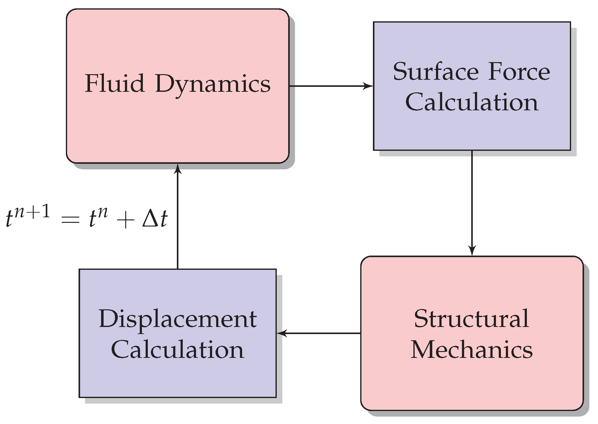
The dynamics of the fluid and solid phases were coupled herein via a co-simulation strategy for both the Eulerian and Lagrangian approaches. The two-way coupling was implemented in two stages as shown in Figure 1: (1) before each time step of the solid phase solver, the forces due to interaction with the fluid were imposed on each solid object as external forces; and (2) after each time step of the solid solver, the position and velocity of the solid phase objects were reported to the fluid solver to provide boundary conditions.

4. Results and Discussion

The Eulerian and Lagrangian approaches were compared and contrasted using four tests. The first test pertains to the flow around a cylinder, a widely used single-phase CFD benchmark problem. A dam break test was used to gauge performance for free-surface flows. Lastly, the two approaches were compared in conjunction with two FSI problems—one pertaining to a floating rigid body and one that had the fluid interacting with an elastic/deformable gate. All the fluid–solid interactions presented below are according to the two-way coupling scheme described in Figure 1.

4.1. Flow around Cylinder—Single-Phase Internal Flow

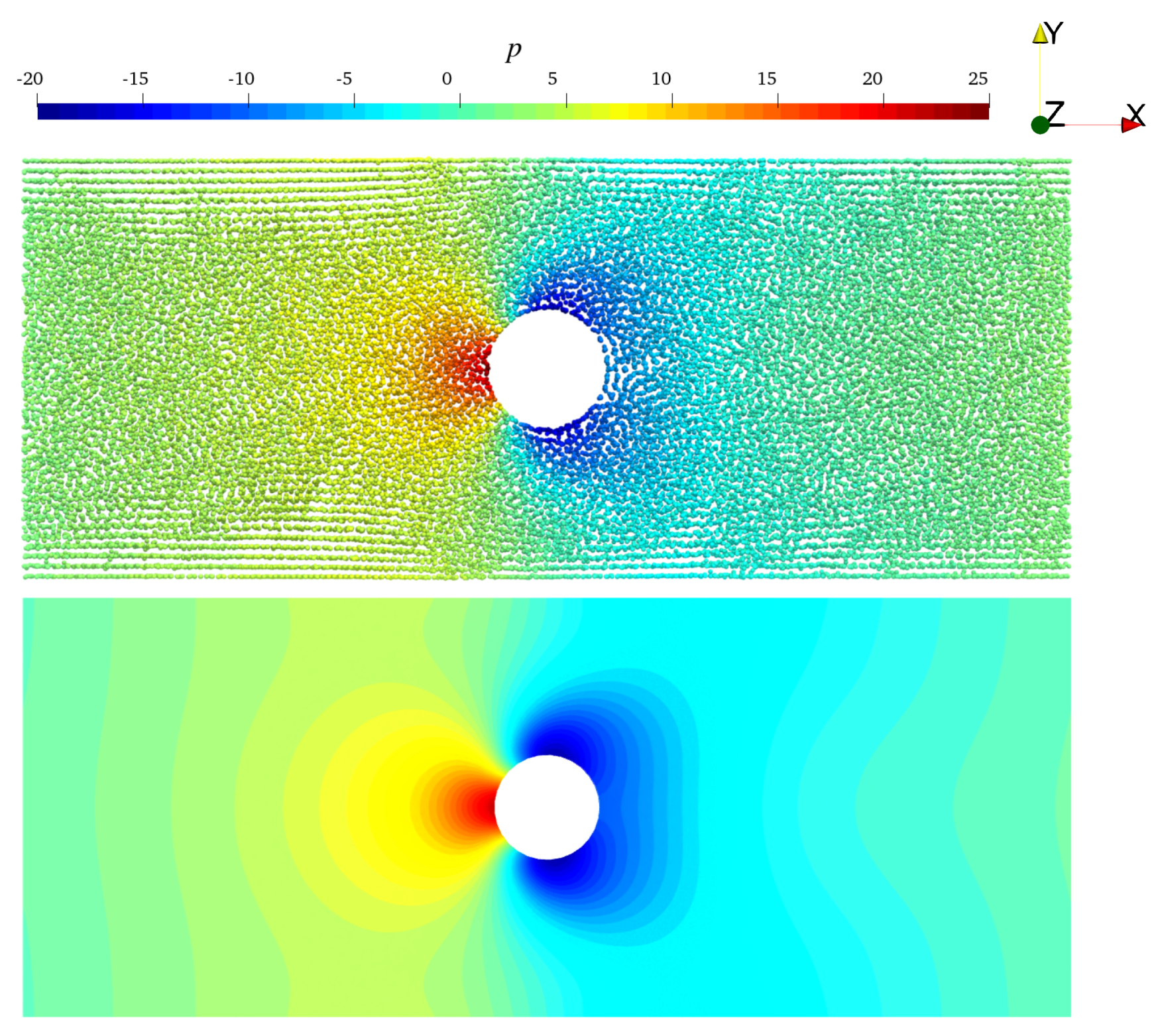
This single-phase, internal flow test was used to compare the FE and SPH solutions for a benchmark problem where the flow is shaped by the interplay between the pressure gradient and the viscous and body forces. The description of the problem geometry and boundary conditions is as follows. The cylinder of diameter $D=0.1$ $\mathrm{m}$ was positioned at the center of a rectangular domain of height 0.4 $\mathrm{m}$ and length 1.0 $\mathrm{m}$ and was fixed. No-slip boundary conditions were applied to the cylinder and the top and bottom walls, while periodic (cyclic) conditions were maintained at the left (inlet) and right (outlet) patches. A constant body force ${\mathbf{f}}_b=1.0$ $\mathrm{m}/{\mathrm{s}}^2$ was applied in the x direction in order to balance the viscous force. The density and viscosity were set to ${\rho }_0=20.0$ $\mathrm{kg}/{\mathrm{m}}^3$ and $\mu =0.1$ $\mathrm{Pa}·\mathrm{s}$, respectively. The grid generated for the FE simulation contained 8 k triangles. The mesh independence study showed a negligible difference in the drag coefficient after increasing the number of triangle from 32 k to 200 k—see Figure 2. We used the same characteristic length and spacing in the SPH simulation as the characteristic triangle size in FE; in this case, $h=0.01$ $\mathrm{m}$ was chosen for the SPH simulation. As illustrated in Figure 3, the steady-state = velocity predicted by SPH and FEM were qualitatively in close agreement. Note that the difference in the appearance of the plots was not quantitative. Indeed, the “dotted-like” look of the SPH plots was a consequence of the Lagrangian nature of the SPH solution in which field values (velocity, in this case) are provided at the location of markers that convect with the flow. Note that the FEM and SPH pressure profiles also showed close agreement as illustrated in Figure 4.

Lastly, we compared the two methods in terms of the drag force. For the drag coefficient, the expression used was $C_d=\frac{F_d}{0.5\rho A{U}^2}$, where $F_d$ is the drag force magnitude along the x axis, $\rho ={\rho }_0$ and $U=1.5$ $\mathrm{m}/\mathrm{s}$ are the reference density and velocity, and $A=wD$ is the frontal area of the cylinder, where w is the width of the cylinder. As shown in Figure 2, SPH and FEM showed different drag coefficients at the onset of the simulation, yet the steady state solutions were in good agreement. We posit that two reasons contributing to these discrepancies were: (i) the different time-integration schemes and (ii) the vastly different space discretization technique and boundary-condition enforcement used in the formulations. The IB method requires a fine mesh near the solid level-set (cylinder) for accurate representation of the fluid-structure interface and forces. Handling this interface poses no major challenge to SPH or boundary-fitted mesh-based approaches, owing to the explicit representation of the fluid-structure interface.

4.2. Dam Break—Two-Phase Free-Surface Flow

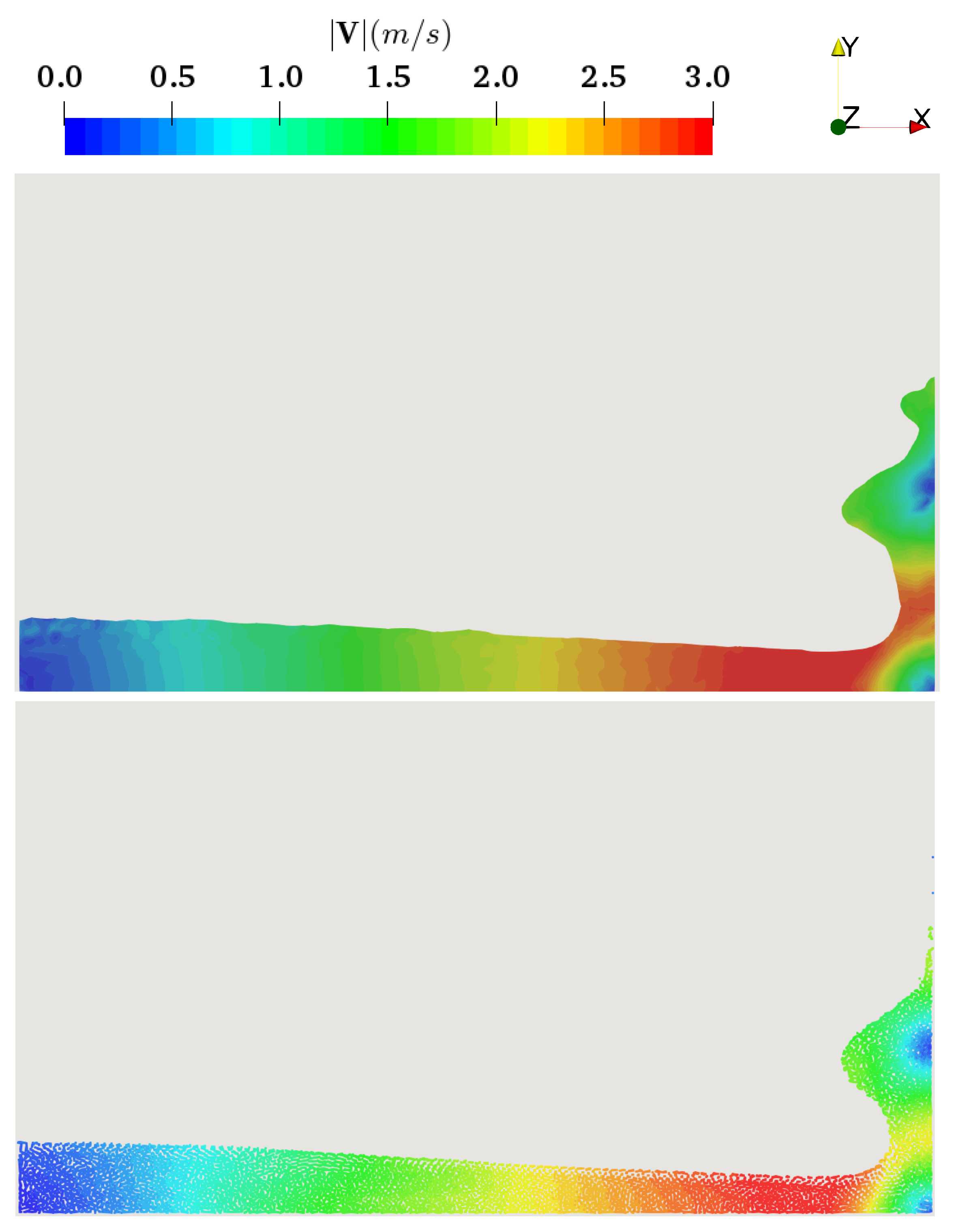
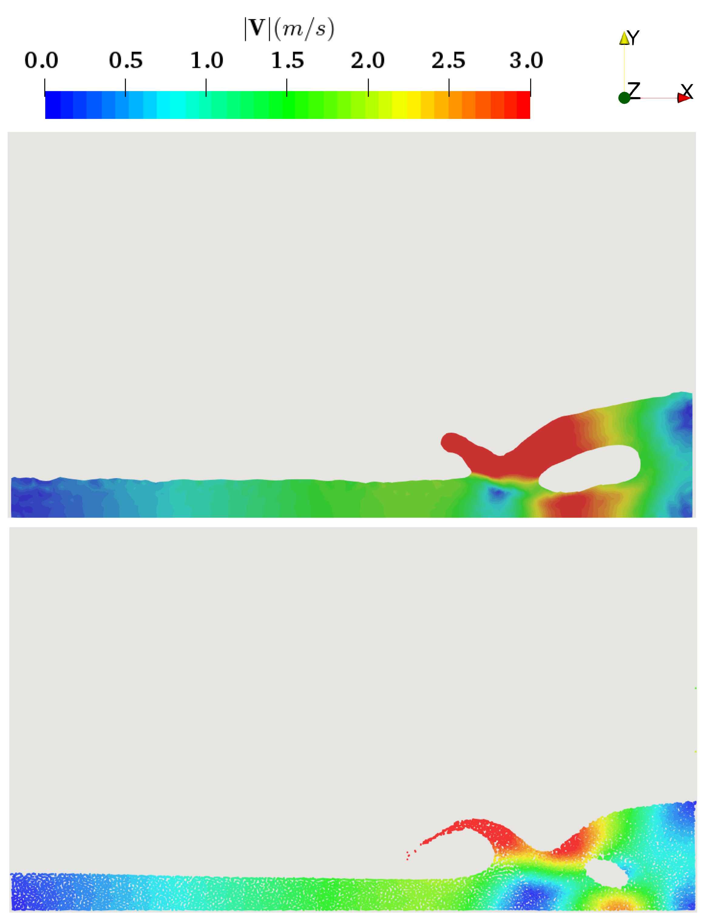
We used the classical dam break problem to demonstrate FE and SPH for free-surface problems. The description of the problem geometry and initial and boundary conditions is as follows. The initial condition and the geometry of the problem is illustrated in Figure 5. The reference density of the air and water domains were ${\rho }_a=1.2$ $\mathrm{kg}/{\mathrm{m}}^3$ and ${\mu }_a=$$1.8\times {10}^{-3}$ Pa·s and ${\rho }_w=1000$ $\mathrm{kg}/{\mathrm{m}}^3$ and ${\mu }_w=$$1\times {10}^{-3}$ Pa·s, respectively. The gravity $g=-9.8$ $\mathrm{m}/{\mathrm{s}}^2$ was applied in the y direction. The initial velocity of the fluid was set to zero everywhere, and the pressure was initialized via a hydrostatic distribution. The wall boundary condition, i.e., the no-slip for velocity and the Neumann boundary $\nabla p·\mathbf{n}=\mathbf{0}$ for pressure, was applied to all solid boundaries. For volume fraction $\theta$, a zero Dirichlet boundary condition was used on the top boundary (and open boundaries in general), while a zero Neumann condition was applied to other boundaries. Note that the air physical properties are only used in the FEM simulation given the two-phase methodology described above. In the SPH simulation, only the water properties were employed, and the effect of the surrounding air was neglected. The SPH and FEM results were compared from two perspectives: (i) the fluid front position over time and (ii) the roll up and the second splash—two characteristics highlighted in previous studies [38,41]. As shown in Figure 6, the SPH solution of the fluid front position over time slightly under-estimated the FEM solution. SPH had an easier task in handling the free-surface since in the Lagrangian framework solving the Navier–Stokes equation (Equation (3)) automatically provides for a tracking of the free-surface [39,41,42,43,44]. In contrast, the Eulerian framework calls for four additional equations: (i) the advection of the level-set field via the velocity (Equation (7)); (ii) the conservation of the volume fraction (Equation (8)); (iii) level-set correction (Equation (14)); and (iv) the mass correction (Equation (12)). This adds significantly to the complexity of the Eulerian solution, a drawback that might be eliminated in the future given that very recent work demonstrates that this multistage algorithm can be collapsed into a single stage [45].

With regard to the roll-up and second splash characteristics, both methods predicted well these two hallmark features of the dam break experiment—see Figure 7 and Figure 8—where the results reported were $1.75$ and $2.05$ s into the simulation.

4.3. Falling Cylinder—Two-Phase Fluid and Rigid–Solid Interaction

This experiment was used to compare the Eulerian and Lagrangian approaches in conjunction with a 3D scenario that displayed ample fluid–solid boundary movement. It may be regarded as a simplified problem that, in more complex forms, is conspicuous in several fluid–structure interaction applications in coastal and offshore structures, e.g., renewable energy devices and caissons. Insofar as the solution methodology is concerned, the test assesses the robustness of the fluid–structure coupling methodology described in Section 3.3.3.

The description of the problem geometry and initial and boundary conditions is as follows. A cylindrical object of radius $r=0.12$ $\mathrm{m}$ and length $L=0.2$ $\mathrm{m}$ was released from the height $h=0.25$ $\mathrm{m}$ above the surface of a tank of water at $t=0$ $\mathrm{s}$. The dimension of the fluid domain was 1.0 $\mathrm{m}$× 1.0 $\mathrm{m}$× 0.2 $\mathrm{m}$ (width × height × depth). The gravity $g=-9.8$ $\mathrm{m}/{\mathrm{s}}^2$ was applied in the y direction. The reference density of the air and water domains were ${\rho }_a=1.2$ $\mathrm{kg}/{\mathrm{m}}^3$ and ${\mu }_a=$$1.8\times {10}^{-3}$Pa·s and ${\rho }_w=1000$ $\mathrm{kg}/{\mathrm{m}}^3$ and ${\mu }_w=$ $1\times {10}^{-3}$Pa·s, respectively. The density of the cylinder was ${\rho }_s=0.7{\rho }_w$, which turned it into a floating structure. The wall boundary conditions were applied to the bottom and side walls of the container and the cylinder. Note that, similar to the dam break problem, the SPH simulation employed a single-phase model neglecting the effect of the surrounding air. Figure 9 illustrates the distribution of the pressure in the frontal cross-section of the domain at $t=0.5$ $\mathrm{s}$.

The cylinder oscillates until its initial potential energy damps out. The steady-state solution of this problem is given by Newton’s second law and basic hydrostatics. Indeed, the upward buoyant force exerted on the body should balance the weight of the object; i.e., ${\rho }_{s}gV=62.0$. Figure 10 illustrates the vertical component of the fluid–structure interaction forces obtained with FEM and SPH and the fact that both methods close in on the steady-state solution approximately 6 s into the simulation. Although the two models showed similar characteristics and steady-state configuration for the vertical force, the SPH solution damped out the oscillation faster due to (i) more numerical damping and, more importantly, (ii) a tighter connection between the fluid and the structure degrees of freedom demonstrated by denser system matrices. Specifically, the FEM fluid-structure force uses the smoothed Heaviside and Dirac delta functions (see Equation (13)). This smoothing is numerically done along $h_e<ϵ<2h_e$ in the mesh where $h_e$ is the element’s characteristic length scale. Incorporating the information from nodes further away at any point requires increasing this smoothing length, which consequently deteriorates the accuracy of the numerical fluid-structure forces.

4.4. Flexible Gate—Two-Phase Fluid and Flexible-Solid Interaction

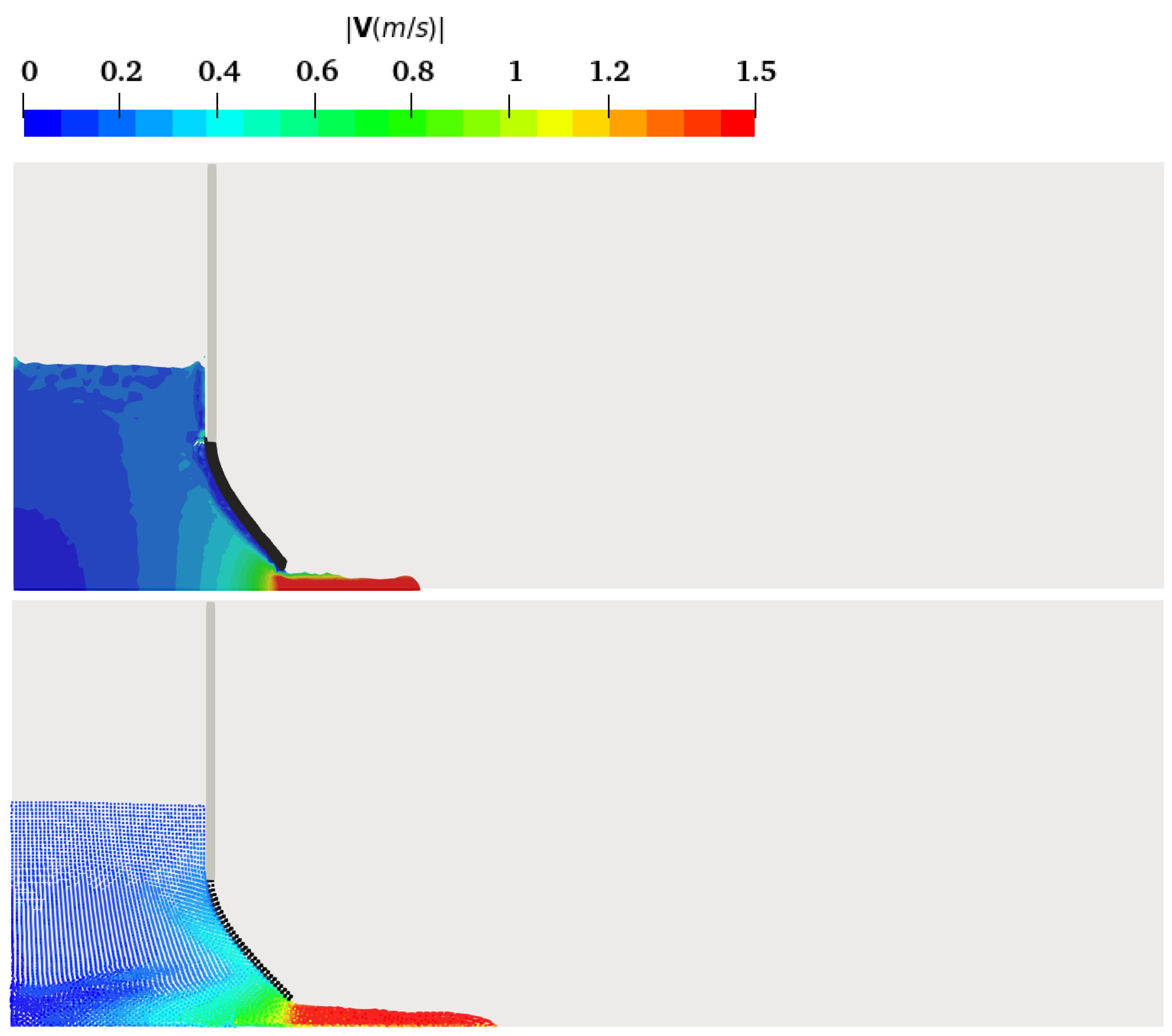
In this experiment [46,47], water was stored in a cubic container that had three rigid vertical sides, while the fourth one was partially made up of a rectangular elastic rubber gate, see the specifications of the elastic gate experiment and the schematic of the initial configuration in Figure 11. The elastic gate, which experienced large deformations, was simulated using a non-linear finite element method called the Absolute Nodal Coordinate Framework (ANCF) [48]. The details about the gradient-deficient ANCF element used herein fall outside of the scope of this contribution but may be found in [49].

Due to the hydrostatic pressure, the elastic gate gradually deflects, and the water exits the tank as shown in Figure 12.

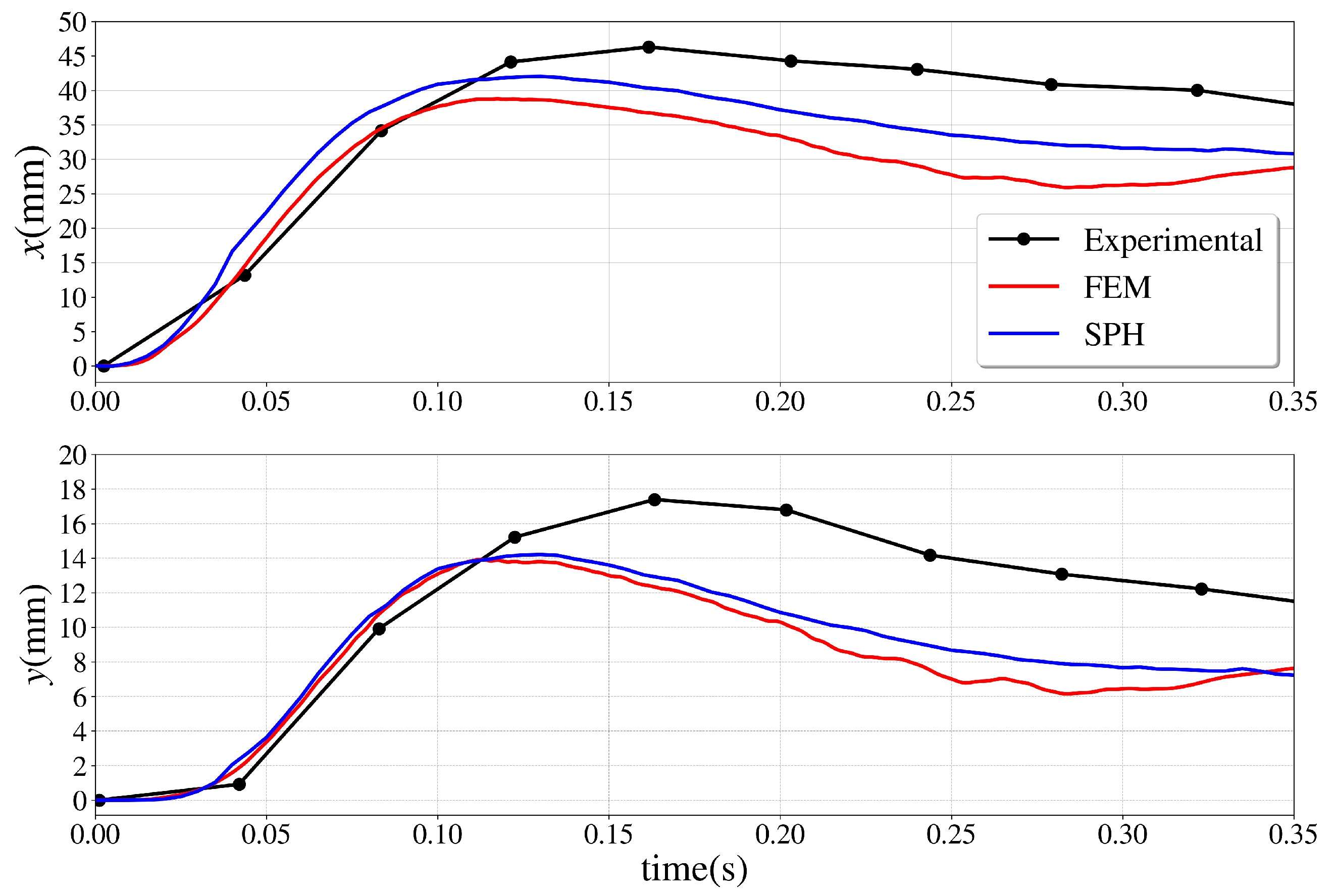
The position of the tip of the gate was measured in the experiment reported in [46]. As shown in Figure 13, the simulation results of both SPH and FEM under-predict the deformation results reported in [46] but are consistent with numerical results reported in [47].

Finally, to provide a general understanding of where both methods stand in terms of computational costs, we present a comparison of the run time of each simulation. Making a fair and conclusive comparison, however, is more challenging than it may appear. Firstly, our Lagrangian and Eulerian packages employ different hardware architectures; the SPH simulations reported below ran on an Nvidia RTX2080 GPU, while the FEM simulations ran on an Intel 3.60GHz core i9-9900K CPU. This is because the parallelism paradigm of the former maps well with the SPH method, whereas the latter is more suitable for Eulerian methods. Second, making a comparison in terms of computation domains is biased and cannot be accurately generalized depending on the problem type. For instance, solving a free-surface problem via a single-phase SPH model is less costly than FEM because the FEM solver in our study has to solve for two phases, i.e., the smaller the size of the fluid domain compared to the overall problem domain, the larger the computational advantage of the SPH approach (even for a similar resolution). Therefore, our choice of the computational domains was based on producing similar-quality results, rather than matching the number of degrees of freedom. Third, the required spatial order of accuracy can change the scenarios toward one or the other method. Computation cost was more favorable for FEM schemes if one employs spatially higher-order accurate methods, as achieving the same goal with SPH requires either increasing the number of interacting neighbor particles, which increases matrices’ sparsity and/or solving local systems per particle for correction matrices. Forth, numerical tolerances and stopping criteria chosen for the methods cannot be directly compared. For instance, in our experience, solving the pressure Poisson equation requires tighter tolerance in FEM compared to SPH. Early stopping in SPH has been shown in previous works [50] to be beneficial in terms of smoothness of the pressure/density field. Last but not least, both of our solvers are research-oriented codes that have great potential for further optimization. All being considered, we provide the computation time of each simulation in

Table 1. Computation time of Eulerian and Lagrangian methods (in seconds) for 1000 time steps of each simulation.

Simulation	SPH Time (# Markers, # Neighbors per Marker)	FEM Time (# Triangles)
Flow around cylinder	233/2900 (42 k, 27/93)	1049/2797 (8 k/32 k)
Dam break	151/486 (54 k, 27/93)	577/5448 (9 k/20 k)
Falling cylinder	464 (115 k, 27)	622 (115 k markers)
Flexible gate	1652 (328 k, 27)	6812 (16 k markers)

for completeness, noting that they should be taken with a grain of salt.

5. Conclusions

We report the results of a study that compared and contrasted the Eulerian and Lagrangian approaches for the solution of free-surface and fluid–solid Interaction (FSI) problems. The two approaches were implemented in two open-source and publicly available codes—Proteus and Chrono—which embrace FEM-based and SPH-based solutions, respectively. Four tests were considered in this study: flow-around-a-cylinder, dam-break, falling-yet-floating-cylinder-in-a-fluid-tank, and elastic-gate problems. We conclude that the SPH methodology is permissive and expeditious. When compared to a more robust Eulerian method such as FEM, the GPU-parallelized SPH solver delivers a solution that is reasonably accurate, computationally less demanding, and easier to produce for the class of problems investigated in this work. The FEM solver is more accurate as are the methods it draws on.

Solving fluid–solid interaction problems of practical relevance remains a challenging undertaking that usually draws on the interplay of complex modeling, numerical algorithms, and software solution techniques. In this context, our goal was that of gaining insights into how the Eulerian and Lagrangian approaches dictate the quality of the FSI numerical solution, which touches on ease of simulation setup as well as solver robustness and efficiency. The two solutions considered herein are polar opposites since the dynamics of the fluid phase were resolved via vastly different space and time discretization techniques as well as software implementations. Indeed, the Lagrangian, SPH-based solver in Chrono condenses the non-linear velocity advection term present in the momentum conservation of the Eulerian formulation (Equation (4)) into the material derivative (Equation (3)). Moreover, the Lagrangian description (Equations (48) and (49)) embraced in Chrono renders the system of equations linear with respect to the velocity unknown. Consequently, the most demanding stage of the Chrono implementation calls at each time step for the solution of a linear system for pressure and velocities. In contrast, the FEM solution in Proteus builds off a more involved implementation that considers additional equations that capture the fluid–solid interface; i.e., the level set advection (Equation (7)) and the volume fraction conservation (Equation (8)). Since the solution of Equation (7) does not guarantee that the new level set is a sign distance function, the level set field needs to be re-initialized (Equation (14)). A mass conservation correction is also required (Equation (12)). The non-linearity associated with the advection term is resolved by using the previous time-step velocity. Nonetheless, even if a projection method is used to decouple pressure and velocity and linearize the Navier–Stokes equation, the mass conservation equation remains non-linear. All things considered, the FEM solver is more sophisticated and computationally demanding. This is because: (i) more equations need to be solved in the FEM solver and (ii) the FEM solver calls for the solution of a non-linear system, which requires the derivation of Jacobian and residual terms. Regarding the parallelization of the solvers, the SPH solver leveraged GPU computing through CUDA, which is suitable for the fine grain parallelization required in SPH. The FEM solver used a distributed memory multi-core parallel implementation via the Message Passing Interface (MPI).

The quality of the pressure field was superior in the FEM solution. Obtaining the correct smooth and accurate field in SPH is more challenging. For instance, if one uses the classical weakly compressible SPH solver that is widely employed in the community but which was not considered herein, the pressure field will experience severe checker-boarding patterns. This can be traced back to the use of a stiff equation of state for evaluating the pressure field, as well as to the decoupling of the velocity and pressure fields—aspects that do not plague the implicit SPH solution discussed herein. The implicit SPH formulation, although more robust than the weakly compressible alternative, may still show checker-boarding effects in highly transient problems where the density of individual particles drops below the rest density. In such cases, the free-surface boundary condition for pressure ($p=0$) kicks in and causes a zigzagging pressure field in the neighborhood of the particles with low density. The checker-boarding artifact has been fixed in Eulerian methods such as the FD method by using staggered grids. The same artifact is avoided on collocated grids in the FV method by Rhie–Chow-type algorithms. FE overcomes this artifact by requiring a mixed FE space seen in the Taylor–Hood elements, in which a lower order approximation space is used for pressure compared to velocity.

Regarding the solution robustness and flexibility, the FEM solver is more robust insofar as the fluid handling is concerned since it takes advantage of the good accuracy and stability of established Eulerian methods. It also allows for a richer set of boundary condition types and flow regimes. On the other hand, the SPH solver in our experience is more robust when dealing with the class of FSI problems studied herein. This is mainly due its Lagrangian framework that lends itself well to the coupling between the fluid and solid phases.

References

- Evans, M.W.; Harlow, F.H.; Bromberg, E. The Particle-in-Cell Method for Hydrodynamic Calculations; Technical Report; Los Alamos National Lab. N. Mex.: Oak Ridge, TN, USA, 1957. [Google Scholar]
- Lucy, L.B. A numerical approach to the testing of the fission hypothesis. Astron. J. 1977, 82, 1013–1024. [Google Scholar] [CrossRef]
- Gingold, R.A.; Monaghan, J.J. Smoothed particle hydrodynamics-theory and application to non-spherical stars. Mon. Not. R. Astron. Soc. 1977, 181, 375–389. [Google Scholar] [CrossRef]
- Monaghan, J.J. Smoothed Particle Hydrodynamics. Rep. Prog. Phys. 2005, 68, 1703–1759. [Google Scholar]
- Trask, N.; Maxey, M.; Hu, X. Compact moving least squares: An optimization framework for generating high-order compact meshless discretizations. J. Comput. Phys. 2016, 326, 596–611. [Google Scholar]
- Hu, W.; Trask, N.; Hu, X.; Pan, W. A spatially adaptive high-order meshless method for fluid–structure interactions. Comput. Methods Appl. Mech. Eng. 2019, 355, 67–93. [Google Scholar] [CrossRef] [Green Version]
- Trask, N.; Maxey, M.; Hu, X. A compatible high-order meshless method for the Stokes equations with applications to suspension flows. J. Comput. Phys. 2018, 355, 310–326. [Google Scholar] [CrossRef] [Green Version]
- Kansa, E.; Multiquadrics, A. A scattered data approximation scheme with applications to computational fluid dynamics. I. Surface approximations and partial derivative estimates. Comput. Math. Appl. 1990, 19, 9. [Google Scholar] [CrossRef] [Green Version]
- Tezduyar, T.E. Interface-tracking and interface-capturing techniques for finite element computation of moving boundaries and interfaces. Comput. Methods Appl. Mech. Eng. 2006, 195, 2983–3000. [Google Scholar] [CrossRef]
- Hirt, C.; Nichols, B. Volume of fluid (VOF) method for the dynamics of free boundaries. J. Comput. Phys. 1981, 39, 201–225. [Google Scholar] [CrossRef]
- Sussman, M.; Smereka, P.; Osher, S. A Level Set Approach for Computing Solutions to Incompressible Two-Phase Flow. J. Comput. Phys. 1994, 114, 146–159. [Google Scholar] [CrossRef]
- Sussman, M.; Puckett, E.G. A Coupled Level Set and Volume-of-Fluid Method for Computing 3D and Axisymmetric Incompressible Two-Phase Flows. J. Comput. Phys. 2000, 162, 301–337. [Google Scholar] [CrossRef] [Green Version]
- Hirt, C.W.; Amsden, A.A.; Cook, J. An arbitrary Lagrangian-Eulerian computing method for all flow speeds. J. Comput. Phys. 1974, 14, 227–253. [Google Scholar] [CrossRef]
- Peskin, C.S. Numerical analysis of blood flow in the heart. J. Comput. Phys. 1977, 25, 220–252. [Google Scholar] [CrossRef]
- Tagliafierro, B.; Mancini, S.; Ropero-Giralda, P.; Domínguez, J.M.; Crespo, A.J.C.; Viccione, G. Performance Assessment of a Planing Hull Using the Smoothed Particle Hydrodynamics Method. J. Mar. Sci. Eng. 2021, 9, 244. [Google Scholar] [CrossRef]
- Fatehi, R.; Manzari, M.T. Error estimation in smoothed particle hydrodynamics and a new scheme for second derivatives. Comput. Math. Appl. 2011, 61, 482–498. [Google Scholar] [CrossRef]
- Libersky, L.; Petschek, A.; Carney, T.; Hipp, J.; Allahdadi, F. High Strain Lagrangian Hydrodynamics: A Three-Dimensional SPH Code for Dynamic Material Response. J. Comput. Phys. 1993, 109, 67–75. [Google Scholar] [CrossRef]
- Randles, P.W.; Libersky, L.D. Smoothed Particle Hydrodynamics: Some recent improvements and applications. Comput. Methods Appl. Mech. Eng. 1996, 139, 375–408. [Google Scholar] [CrossRef]
- Trask, N.; Kim, K.; Tartakovsky, A.; Perego, M.; Parks, M.L. A Highly-Scalable Implicit SPH Code for Simulating Single- and Multi-Phase Flows in Geometrically Complex Bounded Domains; Technical Report; Sandia National Lab. (SNL-NM): Albuquerque, NM, USA, 2015. [Google Scholar]
- Islam, M.R.I.; Chakraborty, S.; Shaw, A. On consistency and energy conservation in smoothed particle hydrodynamics. Int. J. Numer. Methods Eng. 2018, 116, 601–632. [Google Scholar] [CrossRef]
- Kees, C.E.; Farthing, M.W.; Dimakopoulos, A.; de Lataillade, T.; Akkerman, I.; Ahmadia, A.; Bentley, A.; Yang, Y.; Cozzuto, G.; Zhang, A.; et al. erdc/proteus: 1.8.0. 2019. Available online: https://zenodo.org/record/5111912#.Ya1b7rzMKis (accessed on 25 November 2021).
- Tasora, A.; Serban, R.; Mazhar, H.; Pazouki, A.; Melanz, D.; Fleischmann, J.; Taylor, M.; Sugiyama, H.; Negrut, D. Chrono: An open source multi-physics dynamics engine. In High Performance Computing in Science and Engineering—Lecture Notes in Computer Science; Kozubek, T., Ed.; Springer: Berlin/Heidelberg, Germany, 2016; pp. 19–49. [Google Scholar]
- Gurtin, M.E.; Fried, E.; Anand, L. The Mechanics and Thermodynamics of Continua; Cambridge University Press: Cambridge, UK, 2010. [Google Scholar]
- Kees, C.; Akkerman, I.; Farthing, M.; Bazilevs, Y. A conservative level set method suitable for variable-order approximations and unstructured meshes. J. Comput. Phys. 2011, 230, 4536–4558. [Google Scholar] [CrossRef]
- van der Pijl, S.P.; Segal, A.; Vuik, C.; Wesseling, P. A mass-conserving Level-Set method for modelling of multi-phase flows. Int. J. Numer. Methods Fluids 2004, 47, 339–361. [Google Scholar] [CrossRef]
- Burman, E.; Claus, S.; Hansbo, P.; Larson, M.G.; Massing, A. CutFEM: Discretizing Geometry and Partial Differential Equations. Int. J. Numer. Methods Eng. 2015, 104, 472–501. [Google Scholar] [CrossRef] [Green Version]
- Ji, H.; Chen, J.; Li, Z. A New Augmented Immersed Finite Element Method without Using SVD Interpolations. Numer. Algorithms 2016, 71, 395–416. [Google Scholar] [CrossRef]
- Arnold, D.N. Mixed finite element methods for elliptic problems. Comput. Methods Appl. Mech. Eng. 1990, 82, 281–300. [Google Scholar] [CrossRef] [Green Version]
- Ern, A.; Guermond, J.L. Theory and Practice of Finite Elements; Springer: New York, NY, USA, 2004. [Google Scholar] [CrossRef]
- Guermond, J.L.; Salgado, A. A splitting method for incompressible flows with variable density based on a pressure Poisson equation. J. Comput. Phys. 2009, 228, 2834–2846. [Google Scholar] [CrossRef]
- Hu, W.; Pan, W.; Rakhsha, M.; Negrut, D. An Overview of an SPH Technique to Maintain Second-Order Convergence for 2D and 3D Fluid Dynamics; Technical Report TR-2016-14; Simulation-Based Engineering Laboratory, University of Wisconsin-Madison: Madison, WI, USA, 2016. [Google Scholar]
- Chorin, A.J. Numerical solution of the Navier-Stokes equations. Math. Comput. 1968, 22, 745–762. [Google Scholar]
- Asai, M.; Aly, A.M.; Sonoda, Y.; Sakai, Y. A stabilized incompressible SPH method by relaxing the density invariance condition. J. Appl. Math. 2012, 2012, 139583. [Google Scholar] [CrossRef]
- Hu, H. Direct simulation of flows of solid-liquid mixtures. Int. J. Multiph. Flow 1996, 22, 335–352. [Google Scholar] [CrossRef]
- Peskin, C.S. The immersed boundary method. Acta Numer. 2002, 11, 479–517. [Google Scholar] [CrossRef] [Green Version]
- Glowinski, R.; Pan, T.W.; Hesla, T.; Joseph, D. A distributed Lagrange multiplier/fictitious domain method for particulate flows. Int. J. Multiph. Flow 1999, 25, 755–794. [Google Scholar] [CrossRef]
- Kim, Y.; Peskin, C.S. A penalty immersed boundary method for a rigid body in fluid. Phys. Fluids 2016, 28, 033603. [Google Scholar] [CrossRef]
- Adami, S.; Hu, X.; Adams, N. A generalized wall boundary condition for smoothed particle hydrodynamics. J. Comput. Phys. 2012, 231, 7057–7075. [Google Scholar] [CrossRef]
- Rakhsha, M.; Pazouki, A.; Serban, R.; Negrut, D. Using a half-implicit integration scheme for the SPH-based solution of fluid-solid interaction problems. Comput. Methods Appl. Mech. Eng. 2019, 345, 100–122. [Google Scholar] [CrossRef]
- Pazouki, A.; Negrut, D. A numerical study of the effect of particle properties on the radial distribution of suspensions in pipe flow. Comput. Fluids 2015, 108, 1–12. [Google Scholar] [CrossRef]
- Colagrossi, A.; Landrini, M. Numerical simulation of interfacial flows by smoothed particle hydrodynamics. J. Comput. Phys. 2003, 191, 448–475. [Google Scholar] [CrossRef]
- Martin, J.C.; Moyce, W.J. Part IV. An Experimental Study of the Collapse of Liquid Columns on a Rigid Horizontal Plane. Philos. Trans. R. Soc. A Math. Phys. Eng. Sci. 1952, 244, 312–324. [Google Scholar] [CrossRef]
- Hughes, J.P.; Graham, D.I. Comparison of incompressible and weakly-compressible SPH models for free-surface water flows. J. Hydraul. Res. 2010, 48, 105–117. [Google Scholar] [CrossRef]
- Xu, X.; Deng, X.L. An improved weakly compressible SPH method for simulating free surface flows of viscous and viscoelastic fluids. Comput. Phys. Commun. 2016, 201, 43–62. [Google Scholar] [CrossRef]
- Quezada de Luna, M.; Kuzmin, D.; Kees, C.E. A Monolithic Conservative Level Set Method with Built-in Redistancing. J. Comput. Phys. 2019, 379, 262–278. [Google Scholar] [CrossRef]
- Antoci, C.; Gallati, M.; Sibilla, S. Numerical simulation of fluid–structure interaction by SPH. Comput. Struct. 2007, 85, 879–890. [Google Scholar] [CrossRef]
- Yang, Q.; Jones, V.; McCue, L. Free-surface flow interactions with deformable structures using an SPH–FEM model. Ocean Eng. 2012, 55, 136–147. [Google Scholar] [CrossRef]
- Shabana, A. Dynamics of Multibody Systems; Cambridge University Press: Cambridge, UK, 2013. [Google Scholar]
- Yamashita, H.; Valkeapää, A.I.; Jayakumar, P.; Sugiyama, H. Continuum mechanics based bilinear shear deformable shell element using absolute nodal coordinate formulation. J. Comput. Nonlinear Dyn. 2015, 10, 051012. [Google Scholar] [CrossRef] [Green Version]
- Ihmsen, M.; Cornelis, J.; Solenthaler, B.; Horvath, C.; Teschner, M. Implicit incompressible SPH. IEEE Trans. Vis. Comput. Graph. 2014, 20, 426–435. [Google Scholar] [CrossRef] [PubMed]
Figure 1.
Schematic showing the two-way coupling between the structure and fluid systems.
Figure 2.
Flow around a cylinder—variation of the drag coefficient over time.
Figure 3.
Comparison of the steady-state velocity profiles predicted with SPH (top) and FEM (bottom).
Figure 4.
Comparison of the steady-state pressure profiles predicted with SPH (top) and FEM (bottom).
Figure 5.
The fluid domain in the dam break problem is a rectangular prism of size 2 × 1.0 and is placed on the bottom-left end of the rectangular domain of size 5.3 × 3.0 .
Figure 6.
Comparison of fluid-front propagation between SPH and FEM.
Figure 7.
Comparison of the roll-up () in the dam break—FEM (top) and SPH (bottom).
Figure 8.
Comparison of the second splash () in the dam break—FEM (top) and SPH (bottom).
Figure 9.
Figure 10.
Upward buoyant force imparted over time by the fluid to the floating cylinder.
Figure 11.
Schematic and specifications of the elastic gate experiment. Fluid properties: , . Gate properties: , , , thickness = 0.005 [46].
Figure 12.
Snapshots of the elastic gate simulation with FEM (top) and SPH (bottom). The fluid domain colored according to velocity magnitude. The x axis is horizontal, pointing to the left; the y axis is vertical, pointing up.
Figure 13.
Comparison of the position of the tip of the gate between SPH, FEM, and experimental results [46].