
Transient Electrophoresis of a Cylindrical Colloidal Particle

Faculty of Pharmaceutical Sciences, Tokyo University of Science, 2641 Yamazaki, Noda 278-8510, Chiba, Japan
Fluids 2022, 7(11), 342; https://doi.org/10.3390/fluids7110342
Submission received: 10 October 2022
/
Revised: 26 October 2022
/
Accepted: 28 October 2022
/
Published: 29 October 2022
(This article belongs to the Section Flow of Multi-Phase Fluids and Granular Materials)
Abstract
:We develop the theory of transient electrophoresis of a weakly charged, infinitely long cylindrical colloidal particle under an application of a transverse or tangential step electric field. Transient electrophoretic mobility approaches steady electrophoretic mobility with time. We derive closed-form expressions for the transient electrophoretic mobility of a cylinder without involving numerical inverse Laplace transformations and the corresponding time-dependent transient Henry functions. The transient electrophoretic mobility of an arbitrarily oriented cylinder is also derived. It is shown that in contrast to the case of steady electrophoresis, the transient Henry function of an arbitrarily oriented cylinder at a finite time is significantly smaller than that of a sphere with the same radius and mass density as the cylinder so that a cylinder requires a much longer time to reach its steady mobility than the corresponding sphere.
1. Introduction
Transient electrophoresis is the time-dependent unsteady response of a charged colloidal particle in an electrolyte solution to an applied step electric field [1,2,3,4,5,6,7,8,9,10,11,12,13,14,15,16,17,18,19]. It is often required to determine the time necessary for the velocity of a particle to approach its steady value when an electric field is applied to the particle. This information is of practical importance in the efficient design of systems for measurements of steady-state electrophoresis. Morrison [1,2] and later Ivory [3,4] initiated the theory of transient electrophoresis of a spherical or cylindrical particle. The theory of transient electrophoresis has been advanced significantly by Keh and his coworkers [5,6,7,9,10,14,15,16].
Li and Keh [14], in particular, derived the general expression for the Laplace transform of the transient electrophoretic mobility of a weakly charged infinitely long cylinder with arbitrary double-layer thickness in an applied transverse or tangential step electric field and calculated the transient electrophoretic mobility of the particle by using the numerical inverse Laplace transformation method. This method, however, requires tedious numerical calculation and it is not very convenient for practical purposes.
In a previous paper [18], we have shown that the fundamental electrokinetic equations describing the transient electrophoresis of a spherical colloidal particle are quite similar to those for the dynamic electrophoresis of the spherical particle in an applied oscillating electric field [20]. Indeed, it has been shown that there is a simple correspondence between the Laplace transform of the transient electrophoretic mobility and the dynamic electrophoretic mobility of a charged particle in an electrolyte solution [18]. As in the case of a spherical particle, it will be shown that there is the same correspondence relation between the Laplace transform of the transient electrophoretic mobility of a cylinder and its dynamic electrophoretic mobility [21].
The purpose of the present paper is to develop further the theory of transient electrophoresis of a weakly charged infinitely long cylinder in an applied transverse or tangential step electric field and derive closed-form expressions for the transient electrophoretic mobility of the cylinder without involving numerical inverse Laplace transformations.
2. Theory
Let us consider an infinitely long, cylindrical colloidal particle of mass density ρp, radius a, and zeta potential ζ in an aqueous electrolyte solution of mass density ρo, viscosity η, and relative permittivity εr. The electrolyte consists of N ionic species of valence zi, bulk concentration (number density) ni∞, and drag coefficient λi (i = 1, 2, …, N). We suppose that a step electric field E(t) is suddenly applied transversely or tangentially to the cylinder at time t = 0, viz.,
where Eo is constant and the particle starts to move with an electrophoretic velocity U(t) in the direction parallel to Eo (Figure 1). The transient electrophoretic mobility μ(t) of the particle is defined by U(t) = μ(t)E(t) = μ(t)Eo. The origin of the cylindrical coordinate system (r, θ, z) is held fixed at the center of the particle. We treat the case where (i) the liquid can be regarded as incompressible, (ii) the applied electric field E(t) is weak so that terms involving the square of the liquid velocity in the Navier–Stokes equation can be neglected and the particle velocity U(t) is proportional to E(t), and (iii) the relative permittivity of the particle εp is much smaller than that of the electrolyte solution εr (εp « εr).
2.1. Cylinder in a Transverse Field
We first treat the case where E(t) is perpendicular to the cylinder axis (Figure 1a). The fundamental electrokinetic equations for the liquid flow velocity u(r, t) at position r(r, θ, z) and time t and the velocity vi(r, t) of i th ionic species are given by
where e is the elementary electric charge, k is the Boltzmann constant, T is the absolute temperature, εo is the permittivity of a vacuum, p(r, t) is the pressure, ρel(r, t) is the charge density, ψ(r, t) is the electric potential, FH(t) and FE(t) are, respectively, the hydrodynamic and electric forces acting on the cylinder. Equations (2) and (3) are the Navier–Stokes equation and the equation of continuity for an incompressible flow (condition (i)). The term involving the particle velocity U (t) in Equation (2) arises from the fact that the particle has been chosen as the frame of reference for the coordinate system. Equation (4) states that the flow vi(r, t) of the i th ionic species is caused by the liquid flow u(r, t) and the gradient of the electrochemical potential μi(r, t). Equation (5) is the continuity equation for the i th ionic species. Equation (6) is the equation of the motion of the cylinder per unit length.
The initial and boundary conditions for u(r, t) and vi(r, t) are given by
where is the unit normal outward from the particle surface. Equation (8) states that the slipping plane (at which u(r, t) = 0) is located on the particle surface. Equation (10) follows from the condition that electrolyte ions cannot penetrate the particle surface.
For a weak field E(t), the deviations of nj(r, t), ψ(r, t), and μj(r, t) from their equilibrium values (i.e., those in the absence of E(t)) due to the applied field E(t) are small so that we may write
where the quantities with superscript (0) refer to those at equilibrium, the quantities, with δ referring to the deviations from the corresponding equilibrium values, and is a constant independent of r. It is assumed that the equilibrium concentration obeys the Boltzmann distribution and the equilibrium electric potential satisfies the Poisson-Boltzmann equation, viz.,
with
where y (r) is the scaled equilibrium electric potential, κ is the Debye–Hückel parameter, and 1/κ is the Debye length.
From symmetry, we may write
where E(t) is the magnitude of E(t), h(r, t), and φi(r, t) are functions of r and t. By substituting Equations (11)–(13), (18), and (19) into Equations (2)–(5), we obtain the following equations for h(r):
where
is a differential operator, G(r, t) is defined by
and
is the kinematic viscosity. It follows from Equations (9) and (18) that the transverse transient electrophoretic mobility μ(t) can be obtained by
We solve Equation (20) by introducing the Laplace transforms , , and of h(r, t), G(r, t), and μ⊥(r, t), respectively, which are given by
and the Laplace transform of Equation (26) is
The Laplace transform of
Equation (20) thus gives
By solving Equation (29) and using Equation (28), we obtain the following general expression for
:
where Kn(z) is the n th order modified Bessel function of the second kind.
Now consider the low ζ potential case. In this case, it can be shown that (see Ref. [21])
and Equation (22) becomes
The Laplace transform
of G(r, t) is given by
where the equilibrium electric potential ψ(0)(r) for the low ζ potential case is given by
which is obtained from the linearized Poisson-Boltzmann equation ∆ψ(0)(r) = κ2ψ(0)(r) (see Equation (15)). By substituting Equation (34) into Equation (30), we obtain
which agrees with Li and Keh’s result [14]. Li and Keh [14] obtained the transient electrophoretic mobility μ⊥(t) by using the numerical inverse Laplace transform of Equation (35). This method, however, involves tedious numerical calculations and is not very convenient for practical uses. In order to avoid this difficulty, we employ the same approximation method as used for the static electrophoresis problem [22]. We first note that the integrand in Equation (35) has a sharp maximum around r = a + δ/κ, δ being a factor of order unity. This is because the electrical double layer (of the thickness 1/κ) around the cylinder is confined in the narrow region between r = a and r ≈ a + 1/κ. Since the factor (1 + a2/r2) in the integrand of Equation (35) varies slowly with r as compared with the other factors, one may approximately replace r in the factor (1 + a2/r2) by r = a + δ/κ and take it out before the integral sign. That is, we make the following approximate replacement of the difficult factor (1 + a2/r2) by an r-independent constant factor:
In the static electrophoresis [22,23], we have found that the best approximation can be achieved if δ is chosen to be 2.55/
with negligible errors. We use this choice of δ in the transient electrophoresis problem. By using this approximation, the integration in Equation (35) can be carried out analytically to give
with
We obtain μ⊥(t) from
by using the inverse Laplace transformation, viz.,
where the integration is carried out along the vertical line Re(s) = γ in the complex plane, where γ is large so that all the singularities of lie to the left of the line (γ − i∞, γ + i∞) (Figure 2). Since has a branch point at the origin s = 0, we convert this line integral into a contour integral over a large circle G with a cut along the negative part of the real axis Re(s). Since the integral over the large circle Γ vanishes as its radius R tends to infinity, the line integral is replaced by real infinite integrals along CD and EF together with the contribution from the small circle about the origin s = 0 [24].
By making the change in variables
We obtain from Equation (37) the following expression for μ⊥(t):
with
where Jn(λ) and Yn(λ) are, respectively, the n th order Bessel functions of the first and second kinds. In the limit of t→∞, Equation (41) tends to the transverse steady electrophoretic mobility, viz., [22]
which agrees with the following exact expression with negligible errors [22,23].
Equation (41) is the required approximate expression for the transverse transient electrophoretic mobility
with negligible errors. In the limit of large κa (κa » 1),
which agrees with the results of Morison [2] and Li and Keh [14]. For small κa (κa « 1), Equation (41) reduces to
where γ is Euler’s constant (γ = 0.5772).
2.2. Cylinder in a Tangential Field
We next treat the case where the applied electric field E(t) = (0, 0, E(t)) is parallel to the cylinder axis (Figure 1b). The liquid velocity u(r, t) can be expressed as u = u(0, 0, uz(r, t)). The Navier–Stokes equation for uz(r, t)) is given by
By using the Poisson equation
and integrating Equation (47), we finally obtain the following expression for the Laplace transform
of the transient tangential electrophoretic mobility
:
with
For the low ζ
-potential case, Equation (48) becomes
with
As in the case of , by using the inverse Laplace transform , i.e.,
We obtain the following expression for
:
with
In the limit of t→∞, Equation (53) tends to the tangential steady electrophoretic mobility [22,23], viz.,
In the limit of large κa, Equation (53) tends to
while for small κa, Equation (53) tends to
It should be noticed that as in the case of a sphere [18], there is a simple correspondence between the Laplace transform of the transient mobility of a cylinder and its dynamic mobility. That is, and of the transient electrophoretic mobilities and , respectively, can be obtained from the dynamic electrophoretic mobility and of a cylinder under an oscillating electric field of frequency ω by replacing -iω with s and G(r) by G(r)/s.
3. Results and Discussion
The principal results of the present paper are Equations (41) and (53) for the transverse and tangential transient electrophoretic mobilities, respectively. We define the time-dependent transient Henry function as
We thus obtain
and
As t →∞, the transverse transient Henry functions and given by Equations (60) and (61), respectively, tend to the following steady Henry functions [22]:
Note that Equations (41) and (60) are approximate expressions (with negligible errors) that have been derived from the approximation given by Equation (36), while Equations (53) and (61) are exact results.
It is of interest to note that the ratio of the transient Henry function to the steady Henry function takes the same form for the transverse and tangential transient Henry functions, that is,
and
are the same except for the difference between
and
.
Figure 3
shows some examples of the calculation of (Figure 3a) and (Figure 3b) plotted as a function of κa at several values of scaled time νt/a2 at ρp/ρo = 2.
Figure 3 shows how
and
approach their steady values
and
with time.
In the present paper, we treat an infinitely long cylinder, neglecting the end effects. Sherwood [25] demonstrated that the end effects can be neglected under the condition that the cylinder length is much longer than the double-layer thickness 1/κ, Under this condition, it can also be assumed that there is no interaction between cylinders when we consider a dilute suspension of infinitely long cylinders.
Finally, let us consider a cylindrical particle oriented at an arbitrary angle between its axis and the applied electric field. In the present paper we have treated the two types of fields, that is, transverse and tangential electric fields. When an electric field is applied at an arbitrary angle relative to the cylinder axis, the electrophoretic mobility is given by the weighted average of and . Thus -the transient electrophoretic mobility fav(κa, t) averaged over a random distribution of orientation is given by [26]:
Figure 4 shows some examples of the calculation of fav(κa, t) of an arbitrarily oriented cylinder (solid curves) as a function of κa for several values of scaled time νt/a2 at ρp/ρo = 2 in comparison with the transient mobility fsp(κa, t) of a sphere [18] (dotted curves) with the same radius a and mass density ρp as the cylinder.
It is seen from Figure 4 that the average transient Henry function fav(κa, t) of a cylinder at a finite time is considerably lower than the transient Henry function fsp(κa, t) of a sphere with the same radius a and mass density ρp so that a cylinder requires a much longer time to reach its steady mobility than the corresponding sphere, in contrast to the case of steady electrophoresis, where fav(κa, t) is quite similar to fsp(κa, t).
The shape and size dependence of the steady Henry function decreases as its size relative to the Debye length (1/κ) increases and vanishes in the thin double-layer limit (i.e., in the limit of κa →∞ for a sphere and a cylinder, each with radius a) so that a sphere and a cylinder exhibit the same mobility value as that of a particle with a planar surface. On the other hand, even in this limit, the transient Henry function always depends on the particle shape and size.
The present theory can be extended to other types of applied electric fields. It can be shown that in the case where the applied field is an oscillating electric field with frequency ω (i.e., the applied electric field is proportional to e-iωt), the inverse Laplace transforms and of the transient electrophoretic mobilities and , respectively, can be obtained by replacing s with s-iω in Equations (37) and (50).
4. Conclusions
We developed the theory of transient electrophoresis of a weakly charged, infinitely long cylindrical colloidal particle under an application of a transverse or tangential step electric field. We derived closed-form expressions for the transient electrophoretic mobilities and of a cylinder (Equations (41) and (53)) without involving numerical inverse Laplace transformations and the corresponding time-dependent transient Henry functions and (Equations (60) and (61)). The transient Henry function fav(κa, t) of an arbitrarily oriented cylinder is also derived (Equation (64)). It is shown that in contrast to the case of steady electrophoresis, the transient Henry function fav(κa, t) of an arbitrarily oriented cylinder at a finite time is significantly smaller than the transient Henry function fsp(κa, t) of a sphere with the same radius a and mass density ρp as the cylinder so that a cylinder requires a much longer time to reach its steady mobility than the corresponding sphere. It is also shown that, unlike the steady Henry function, the transient Henry function for a cylinder differs from that of a sphere even in the limit of large κa.
Funding
This research reserved no external funding.
Institutional Review Board Statement
Not applicable.
Informed Consent Statement
Not applicable.
Data Availability Statement
Not applicable.
Conflicts of Interest
The author declares no conflict of interest.
References
- Morrison, F.A. Transient electrophoresis of a dielectric sphere. J. Colloid Interface Sci. 1969, 29, 687–691. [Google Scholar] [CrossRef]
- Morrison, F.A. Transient electrophoresis of an arbitrarily oriented cylinder. J. Colloid Interface Sci. 1971, 36, 139–145. [Google Scholar] [CrossRef]
- Ivory, C.F. Transient electroosmosis: The momentum transfer coefficient. J. Colloid Interface Sci. 1983, 96, 296–298. [Google Scholar] [CrossRef]
- Ivory, C.F. Transient electrophoresis of a dielectric sphere. J. Colloid Interface Sci. 1984, 100, 239–249. [Google Scholar] [CrossRef]
- Keh, H.J.; Tseng, H.C. Transient electrokinetic flow in fine capillaries. J. Colloid Interface Sci. 2001, 242, 450–459. [Google Scholar] [CrossRef] [Green Version]
- Keh, H.J.; Huang, Y.C. Transient electrophoresis of dielectric spheres. J. Colloid Interface Sci. 2005, 291, 282–291. [Google Scholar] [CrossRef]
- Huang, Y.C.; Keh, H.J. Transient electrophoresis of spherical particles at low potential and arbitrary double-layer thickness. Langmuir 2005, 21, 11659–11665. [Google Scholar] [CrossRef]
- Khair, A.S. Transient phoretic migration of a permselective colloidal particle. J. Colloid Interface Sci. 2012, 381, 183–188. [Google Scholar] [CrossRef]
- Chiang, C.C.; Keh, H.J. Startup of electrophoresis in a suspension of colloidal spheres. Electrophoresis 2015, 36, 3002–3008. [Google Scholar] [CrossRef]
- Chiang, C.C.; Keh, H.J. Transient electroosmosis in the transverse direction of a fibrous porous medium. Colloids Surf. A Physicochem. Engin. Asp. 2015, 481, 577–582. [Google Scholar] [CrossRef]
- Saad, E.I.; Faltas, M.S. Time-dependent electrophoresis of a dielectric spherical particle embedded in Brinkman medium. Z. Angew. Math. Phys. 2018, 69, 43. [Google Scholar] [CrossRef]
- Saad, E.I. Unsteady electrophoresis of a dielectric cylindrical particle suspended in porous medium. J. Mol. Liquid 2019, 289, 111050. [Google Scholar] [CrossRef]
- Saad, E.I. Start-up Brinkman electrophoresis of a dielectric sphere for Happel and Kuwabara models. Math. Meth. Appl. Sci. 2018, 41, 9578–9591. [Google Scholar] [CrossRef]
- Li, M.X.; Keh, H.J. Start-up electrophoresis of a cylindrical particle with arbitrary double layer thickness. J. Phys. Chem. B 2020, 124, 9967–9973. [Google Scholar] [CrossRef]
- Lai, Y.C.; Keh, H.J. Transient electrophoresis of a charged porous particle. Electrophoresis 2020, 41, 259–265. [Google Scholar] [CrossRef]
- Lai, Y.C.; Keh, H.J. Transient electrophoresis in a suspension of charged particles with arbitrary electric double layers. Electrophoresis 2021, 42, 2126–2133. [Google Scholar] [CrossRef]
- Sherief, H.H.; Faltas, M.S.; Ragab, K.E. Transient electrophoresis of a conducting spherical particle embedded in an electrolyte-saturated Brinkman medium. Electrophoresis 2021, 42, 1636–1647. [Google Scholar] [CrossRef]
- Ohshima, H. Approximate analytic expression for the time-dependent transient electrophoretic mobility of a spherical colloidal particle. Molecules 2022, 27, 5108. [Google Scholar] [CrossRef]
- Ohshima, H. Transient electrophoresis of a spherical soft particle. Colloid Polym. Sci. 2022, accepted. [Google Scholar] [CrossRef]
- Ohshima, H. Dynamic electrophoretic mobility of a spherical colloidal particle. J. Colloid Interface Sci. 1996, 179, 431–438. [Google Scholar] [CrossRef]
- Ohshima, H. Dynamic electrophoretic mobility of a cylindrical colloidal particle. J. Colloid Interface Sci. 1997, 185, 131–139. [Google Scholar] [CrossRef] [PubMed]
- Ohshima, H. Henry’s function for electrophoresis of a cylindrical colloidal particle. J. Colloid Interface Sci. 1996, 180, 299–301. [Google Scholar] [CrossRef]
- Henry, D.C. The cataphoresis of suspended particles. Part I.-The equation of cataphoresis. Proc. R. Soc. Lond. A 1931, 133, 106–129. [Google Scholar]
- Carslaw, H.S.; Jaeger, J.C. Conduction of Heat in Solids, 2nd ed.; Oxford University Press: Oxford, UK, 1959. [Google Scholar]
- Sherwood, J.D. Electrophoresis of rods. J. Chem. Soc. Faraday Trans. 2 1982, 78, 1091–1100. [Google Scholar] [CrossRef]
- de Keizer, A.; van der Drift, W.P.J.T.; Overbeek, J.T.H.G. Electrophoresis of randomly oriented cylindrical particles. Biophys. Chem. 1975, 3, 107–108. [Google Scholar] [CrossRef]
Figure 1.
Cylindrical colloidal particle of radius a and zeta potential ζ moving with a transient velocity U(t) in an applied step electric field E(t). The electric field E(t) is perpendicular to the cylinder axis (a) or parallel to it (b). U(∞) is the magnitude of U(∞) at t = ∞.
Figure 1.
Cylindrical colloidal particle of radius a and zeta potential ζ moving with a transient velocity U(t) in an applied step electric field E(t). The electric field E(t) is perpendicular to the cylinder axis (a) or parallel to it (b). U(∞) is the magnitude of U(∞) at t = ∞.

Figure 2.
Contour integral on the complex plane of s.
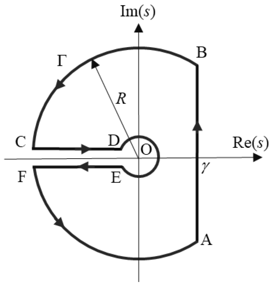
Figure 3.
Time-dependent transient Henry functions (a) and (b) of a cylindrical colloidal particle of radius a and mass density ρp in an electrolyte solution of mass density ρo, kinematic viscosity ν, and Debye–Hückel parameter κ plotted as a function of κa for various values of scaled time νt/a2 at ρp/ρo = 2. The values of and at t → ∞, i.e., and are the steady Henry functions.
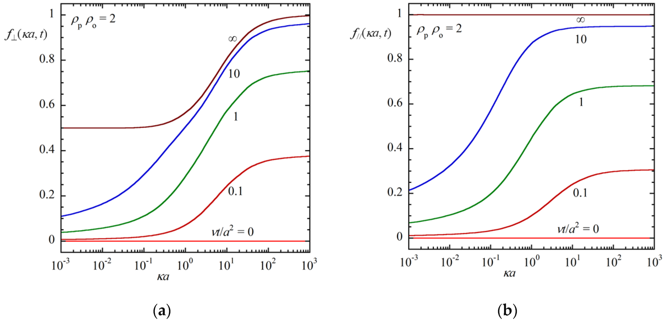
Figure 4.
Time-dependent transient Henry function of an arbitrarily oriented cylinder with radius a and mass density ρp in an electrolyte solution of mass density ρo, kinematic viscosity ν, and Debye–Hückel parameter κ plotted as a function of κa for various values of scaled time νt/a2 at ρp/ρo = 2 (solid curves). The transient Henry function fsp(κa, t) for a sphere [18] is also shown for comparison (dotted curves).

Publisher’s Note: MDPI stays neutral with regard to jurisdictional claims in published maps and institutional affiliations. |
© 2022 by the author. Licensee MDPI, Basel, Switzerland. This article is an open access article distributed under the terms and conditions of the Creative Commons Attribution (CC BY) license (https://creativecommons.org/licenses/by/4.0/).
Share and Cite
MDPI and ACS Style
Ohshima, H. Transient Electrophoresis of a Cylindrical Colloidal Particle. Fluids 2022, 7, 342. https://doi.org/10.3390/fluids7110342
AMA Style
Ohshima H. Transient Electrophoresis of a Cylindrical Colloidal Particle. Fluids. 2022; 7(11):342. https://doi.org/10.3390/fluids7110342
Chicago/Turabian StyleOhshima, Hiroyuki. 2022. "Transient Electrophoresis of a Cylindrical Colloidal Particle" Fluids 7, no. 11: 342. https://doi.org/10.3390/fluids7110342