Experimental and Numerical Study of Cavitation Number Limitations for Hydrodynamic Cavitation Inception Prediction

Abstract

Hydrodynamic cavitation is the formation, growth and subsequent collapse of vapor bubbles in a moving liquid. It is extremely important to determine conditions of cavitation inception and when it starts damaging industrial equipment. In some cases, such as hydrodynamic cleaning it is important to understand how to improve the cavitation phenomenon in order to enhance cleaning properties. The cavitation number is a parameter used to predict cavitation and its potential effects. In this paper we discuss limitations of this parameter and demonstrate that it cannot be considered sufficient to predict cavitation inception and development in the fluid flow. The experimental setup was designed and built to study cavitation inception in various nozzles. RANS SST k–ω turbulence model was used in this study to model turbulent flow in ANSYS Fluent. CFD calculations were compared to experimental results. It was shown that cavitation inception was sensitive to change in nozzle geometry and, since geometrical parameters are not included in cavitation number formula, scenarios of cavitation inception can be different at the same cavitation number.

1. Introduction

Cavitation is a formation of vapor bubbles within a liquid at low-pressure regions. Cavitation can be generated by an ultrasonic acoustic field [1,2] or it can appear in moving fluid, which is the focus of this study. Hydrodynamic cavitation is the formation, growth and subsequent collapse of cavities (bubbles) filled with the mixture of gas and vapor in a moving liquid. This process of bubble formation occurs when the flow rate increases and the pressure in the system approaches the saturated vapor pressure at a given liquid temperature. Collapse of these vapor bubbles leads to the appearance of local microjets and shock waves and, as a result, erosion of surfaces which are in contact with cavitation, noise and vibrations [3]. For many industrial applications it is extremely important to determine conditions at which cavitation will start to form and to damage equipment. In some cases, such as in case of high-pressure hydrodynamic jet, which is used for cleaning pipes from salt deposits with radionuclides [4], cleaning heat exchangers, for the deep hole drilling [5] and many other industrial applications [6], it is important to understand how to improve cavitation phenomenon in order to enhance jet’s erosion properties.

The parameter used to predict cavitation and the potential effects of cavitation (such as erosion) is the cavitation number [7]:

$$\sigma =\frac{P_a-P_v}{\frac{1}{2}\rho v_e^2}$$

(1)

where P_a is an ambient pressure; P_v is a vapor pressure of the liquid; v_e is the mean jet exit velocity; ρ is a liquid density.

Cavitation number can be calculated for any flow, and the cavitation number at which the flow starts to produce cavitation is called critical cavitation number or incipient cavitation number. It can be seen from (1) that if σ is large (large ambient pressure or small flow velocity) there will be no cavitation produced. By increasing flow velocity and decreasing ambient pressure, the cavitation number can be reduced and when it drops to a critical (incipient) value cavitation bubbles will start to appear in the flow. Further reduction of the cavitation number will affect cavitation intensity and cavitation erosion.

For different fluid mechanics processes and different geometries of cavitation chambers, the inception number can be different. In [8], hydrodynamic cavitation technique was tested for the degradation of orange-G dye in the context of degradation of various organic pollutants such as pesticides, pharmaceutical drugs, and textiles dyes. A total of three cavitating devices were used: circular and slit Venturi and an orifice plate. Experiments were performed at different inlet pressures ranging from 3 to 7 bar. There was an observable optimum inlet pressure and cavitation number at which dye decolorization rate was maximum for all three cavitating devices. The optimized inlet pressure was 3 bar with a cavitation number of 0.29 for the slit Venturi, 5 bar with a cavitation number of 0.15 for the circular Venturi and 5 bar with a cavitation number of 0.24 for orifice. Similar experiments with reactive red dye were conducted in [9]. The first clear cavity cloud was observed at 6 bar pressure (cavitation number 0.13) and with further increases in inlet pressure almost the entire downstream area was filled with cavity cloud. In [10], hybrid methods based on cavitation coupled with the Fenton process for the treatment of wastewater were discussed and different types of reactors used for the combined processes were analyzed. In addition, some recommendations for large-scale operation were given. A cavitation number in the range of 0.1 to 1 was reported to be optimal for the reactor’s operations since very low operating cavitation numbers could lead to super-cavitation resulting in vapor cloud formation and no collapse of cavitation bubbles. In [11], a theoretical and experimental study of cavitation as an advanced oxidation process was conducted. The degradation rate of p-nitrophenol (PNP) was experimentally investigated and used as an estimator of the sonochemical effect in hydrodynamic cavitation. A flow was passed through a Venturi tube; an optimal Venturi tube inlet pressure value was found to be 0.4 MPa and optimal cavitation number was 0.25. In [12], degradation of imidacloprid (neonicotinoid class of insecticide) in aqueous solution was studied using hydrodynamic cavitation. A circular Venturi tube was used as hydrodynamic cavitation test chamber. Rate of degradation of imidacloprid using hydrodynamic cavitation was found to be dependent on the following parameters: inlet pressure, cavitation number and pH of the feed solution. An inlet pressure of 15 bar, cavitation number of 0.067 and acidic conditions were recommended for enhancing the extent of degradation of imidacloprid. A low cavitation number ($\sigma =0.08)$ was also observed in [4] in Ba(Ra)SO₄ cleaning application. In [13], hydrodynamic cavitation was studied in different geometries of Venturi tubes and it was shown that the cavitation number could not be used as a single parameter to define cavitation inception and intensity. The self-resonating jet (self-excited pulsed jet) was first proposed and studied in [14,15] (part I and II of the same study). These jets were used for deep hole drilling to accommodate increasing cavitation numbers with increasing depth of drilling. Using fluid dynamics principles for a structured jet, the cavitation number can be defined as follows:

$$\sigma =\frac{{\Gamma }^2}{2{\pi }^2{V}^2{r}_c^2}$$

(2)

where Γ is the circulation around vortex

$$\Gamma ={{\displaystyle \oint }}^{ }v\times ds=V\times \lambda$$

λ is the acoustic wavelength, V—jet velocity, r_c—vortex core radius

In [16], self-resonating cavitating jets were used for bitumen separation from the oil sand and for cavitation erosion study in the multiphase slurry media. The cavitation number was calculated based on (1) as 0.19. In [17], a series of nozzles were designed for low-intensity cavitation at high cavitation numbers ($\sigma$ = 0.37−0.46), calculated based on (1), to test different types of cavitation generators for bitumen separation from the oil sand.

In [18], a fundamental study of the large cavitation bubble dynamics in a tube, filled with degassed water, was studied. Large scale cavitation bubbles were formed on the bottom of the tube when it was driven upwards and hitting the stopper, generating water separation due to inertial water movement. A new cavitation number was proposed to describe the maximum length of cavitation bubble:

$$C_{a2}=l^{*-1}{C}_{a0}$$

(3)

where l* is a non-dimensional length of the water column indicating its slenderness and C_a0 is the classical cavitation number described in (1). Such cavitation number defines appearance of large vapor caverns when $C_{a2}<1$. In [19], it was shown that cavitation could occur at low velocities (on the order of 1 m/s), when a flat-bottomed cylinder impacts onto a liquid pool. Cavitation number (1) was also modified in this case and was introduced as

$$C_a=\alpha M{a}^{-1}$$

(4)

where Ma is the impact Mach number and $\alpha$ is impacting angle and when C_a is sufficiently small (i.e., C_a < k₁, where k₁ is a constant of order unity), cavitation is expected. Another modification of cavitation number was suggested in [20]. The experiment similar to presented in [18] was conducted and proposed dimensionless number was more suitable to predict the cavitation onset caused by a sudden acceleration rather than a large velocity as prescribed by the traditional cavitation number (1). In [21], correlation of bisphenol A (BPA) degradation by hydrodynamic cavitation with the fluid mechanical properties of the cavitating jet in a reactor was studied. The effects of inlet pressure and two orifices were investigated and the fluid mechanics conditions during the reaction were evaluated by optical measurements to determine the jet length, bubble volume, number of bubbles, and bubble size distribution. Cavitation number was calculated based on (1) and was changed from 0.2 to 0.03. In [22], the cavity behavior and its corresponding wall static pressure characteristics in Venturi channels with various divergence angles to research the role of the divergence angle in cavity shape and the wall static pressure oscillation was studied. Five rectangular Venturi channels with different divergence angles (4°, 6°, 8°, 10°, and 12°) were tested at the cavitation number from 0.3 to 1.0.

The first reason of such a wide spread of optimal and operation cavitation numbers are the various applications which require different regimes of cavitation and cavitation efficiency. In addition, the second reason is that all cavitation devices are different and there is no standard set of parameters, used for cavitation number calculations.

In this paper we studied different parameters which affect cavitation inception and development. Different geometries of cavitation chambers were tested and different parameters in the hydraulic system were used to calculate cavitation number. The geometry of cavitation chambers was studied in combination with temperature and pressure variations in the system. It was shown that cavitation number cannot be used as the main hydrodynamic cavitation characteristic since it does not share a connection with the cavitation chamber’s or nozzle’s geometry and it can be calculated in several different ways in the same system, producing different values.

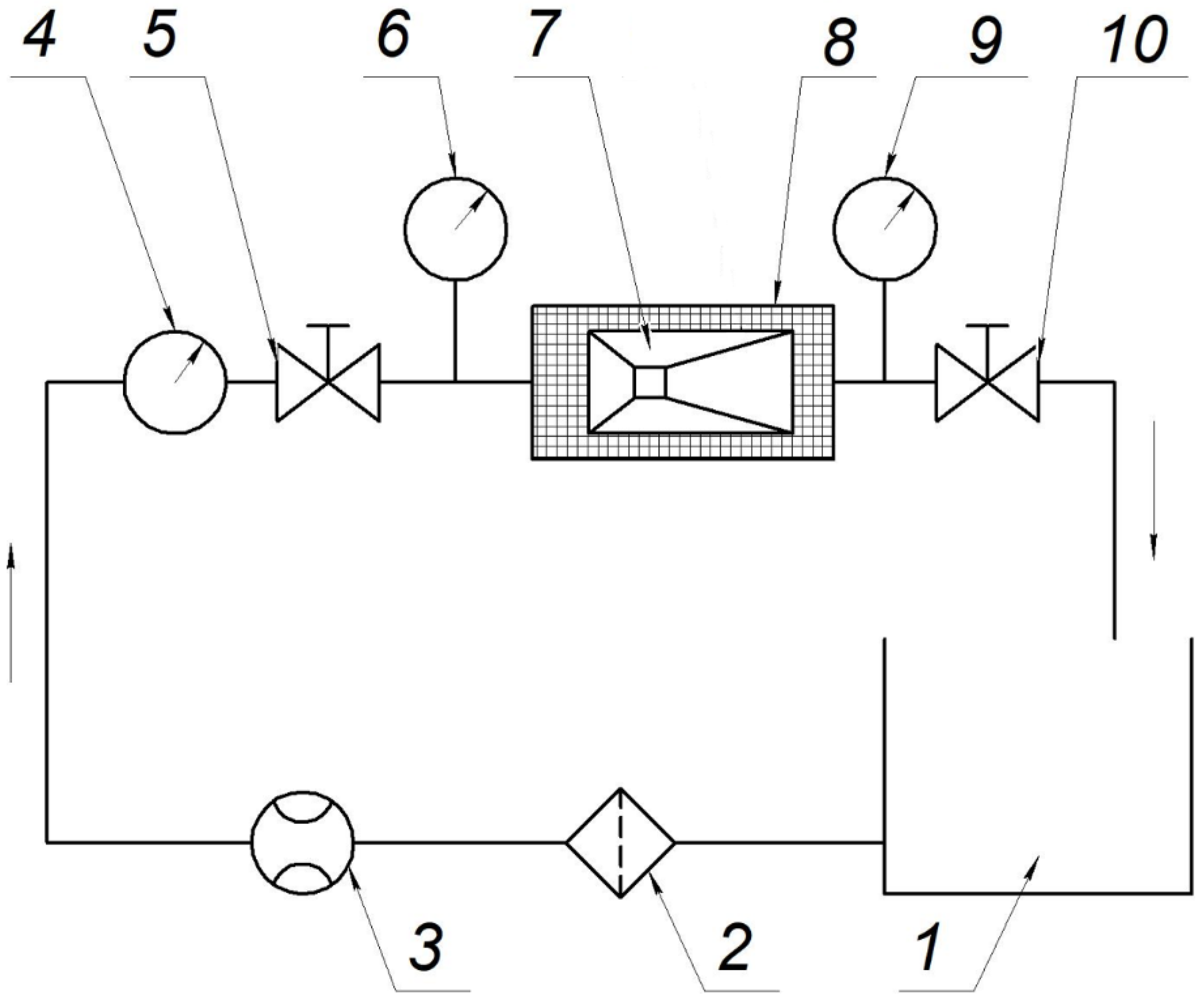
The experimental setup was designed and built to study cavitation inception and development. Turbulent flow was also modeled in ANSYS Fluent and CFD calculations were compared to experimental results.

2. Experimental Procedures

The experimental setup used to study the cavitation is shown in Figure 1. A 7.5 kW centrifugal pump was used to pump the tap water through hydrodynamic loop. Replaceable axisymmetric cavitation generators (cavitators) were made of transparent material (organic glass), for visual detection of cavitation inception. A scale grid with a 1 cm × 1 cm cells was used as a reference to measure cavitation zone size. A microphone was used for acoustic measurements of cavitation noise. All components of the system were connected with 55 mm flexible hoses.

KROHNE electromagnetic flowmeter (accuracy: ±0.2% from 0.031545 m³/s of FS). Bourdon pressure gauges were used for pressure measurements (0–5 bar, ±2% FS).

Three different Venturi tubes configurations were used in this study (Figure 2).

Figure 2a: Venturi tube with 60° reducer, cylindrical part and 13° diffuser.

Figure 2b: Same geometry as in the first case but inverted.

Figure 2c: Cylindrical nozzle.

Figure 2d: Conical 13° diverging nozzle.

The smallest inner flow section diameter for all test chambers was 12 mm, length 150 mm, and outer diameter 40 mm. More detailed geometry is shown in Figure 3.

For each of the test chambers, critical values of the pressure drop for cavitation inception were experimentally determined, as well as the geometric characteristics of cavitation cavities at various pressure parameters.

3. Numerical Method

RANS (Reynolds-averaged Navier–Stokes) SST k–ω turbulence model in the system with Energy Equation was used for CFD analysis. This model was developed by Menter [23] to effectively blend the robust and accurate formulation of the k–ω model in the near-wall region with the free-stream independence of the k–ε model in the far field, which makes it more accurate and reliable for a wider class of flows. Transport Equations (5) and (6) for SST k–ω model has a similar form to the standard k–ω model. The y+ value is a non-dimensional distance (based on local cell fluid velocity) from the wall to the first mesh node. For this model Ansys CFX is using an automatic value for y+ parameter, y+ > 11 for high Reynolds numbers, and y+ < 2 for low Reynolds numbers.

$$\frac{\partial }{\partial t}\left(\rho k\right)+\frac{\partial }{\partial x_i}\left(\rho k{u}_i\right)=\frac{\partial }{\partial x_j}\left({\Gamma }_k\frac{\partial k}{\partial x_j}\right)+\widetilde{G_k}-Y_k+S_k$$

(5)

$$\frac{\partial }{\partial t}\left(\rho \omega \right)+\frac{\partial }{\partial x_i}\left(\rho \omega u_i\right)=\frac{\partial }{\partial x_j}\left({\Gamma }_{\omega }\frac{\partial \omega }{\partial x_j}\right)+G_{\omega }-Y_{\omega }+D_{\omega }+S_{\omega }$$

(6)

where $\widetilde{G_k}$ represents the generation of turbulence kinetic energy due to mean velocity gradients. $G_{\omega }$ represents the generation of ω, ${\Gamma }_k$ and ${\Gamma }_{\omega }$ represent the effective diffusivity of k and ω. $Y_k$ and $Y_{\omega }$ represent the dissipation of k and ω due to turbulence. $D_{\omega }$ represents the cross-diffusion term; $S_k$ and $S_{\omega }$ are user-defined source terms. The cavitation model was represented by the Rayleigh–Plesset equation:

$$R_B\frac{d^2{R}_B}{d{t}^2}+\frac{3}{2}{\left(\frac{d{R}_B}{dt}\right)}^2+\frac{2\sigma }{{\rho }_f{R}_B}=\frac{p_v-p}{{\rho }_f}$$

(7)

where R_B—is the radius of the bubble, p_v—is the pressure in the bubble (vapor pressure at the given temperature of the liquid), p—is the pressure in the liquid surrounding the bubble, ρ_f—is the density of the liquid, and σ—is the coefficient of surface tension between the liquid and vapor. Equation (7) is based on mechanical balance assuming no thermal barriers of bubble growth. Neglecting second-order terms (which is suitable for low vibration frequencies) and surface tension, this equation can be reduced to:

$$\frac{d{R}_B}{dt}=\sqrt{\frac{2}{3}\frac{p_v-p}{{\rho }_f}}$$

(8)

The rate of change in bubble volume is calculated as follows:

$$\frac{d{V}_B}{dt}=\frac{d}{dt}\left(\frac{4}{3}\pi R_B^3\right)=\pi R_B^2\sqrt{\frac{2}{3}\frac{p_v-p}{{\rho }_f}}$$

(9)

and the rate of change in the mass of the bubble is:

$$\frac{d{m}_B}{dt}={\rho }_g\frac{d{V}_B}{dt}=\pi R_B^2{\rho }_g\sqrt{\frac{2}{3}\frac{p_v-p}{{\rho }_f}}$$

(10)

If N_B is the number of bubbles per unit volume, the volume fraction r_g can be expressed as:

$$r_g=V_B{N}_B=\frac{4}{3}\pi R_B^3{N}_B$$

(11)

and the total rate of interfacial mass transfer per unit volume is:

$${\dot{m}}_{fg}=N_B\frac{d{m}_B}{dt}=\frac{3{\rho }_g{r}_g}{R_B}\sqrt{\frac{2}{3}\frac{p_v-p}{{\rho }_f}}$$

(12)

This expression was obtained under the assumption of bubble growth (evaporation). It can be generalized for condensation as follows:

$${\dot{m}}_{fg}=F\frac{3{\rho }_g{r}_g}{R_B}\sqrt{\frac{2}{3}\frac{\left|p_v-p\right|}{{\rho }_f}}sgn\left(p_v-p\right)$$

(13)

where F—an empirical coefficient that can differ for condensation and evaporation, designed to consider the fact that they can occur at different rates (condensation is usually much slower than evaporation). Although Equation (13) has been generalized for evaporation and condensation, it could be further optimized for evaporation process. Evaporation starts at the spots of nucleation (most often non-condensable gases) and r_g in (13) is replaced by 1 − r_g, to obtain:

$${\dot{m}}_{fg}=F\frac{3r_{nuc}{\rho }_g\left(1-r_g\right)}{R_B}\sqrt{\frac{2}{3}\frac{\left|p_v-p\right|}{{\rho }_f}}sgn\left(p_v-p\right)$$

(14)

where r_nuc—volume fraction in nucleation centers. Equation (13) is also preserved in the case of condensation and R_B represents the radius of cavitation bubbles at nucleation.

ANSYS Workbench 21 software package was used for numerical solution of governing equations. Computation domains are shown in Figure 3. Geometrical parameters correspond to geometry of the three types of cavitation test chambers which were used in the experiments (Figure 2). Additional entrance length was not considered. We used normal orientation of the flow with zero gradient as the entrance conditions. All cases were axisymmetric. The solution of the problem in °CFX–Solver, based on the finite-volume method, was performed in two stages. In the first stage, a converged solution was obtained with the cavitation model turned off, then the data were imported into the duplicated CFX solver, and the cavitation flow analysis was performed. Water (incompressible fluid under isothermal flow conditions) was used as a fluid with a reference pressure of 1 atm at 15 °C.

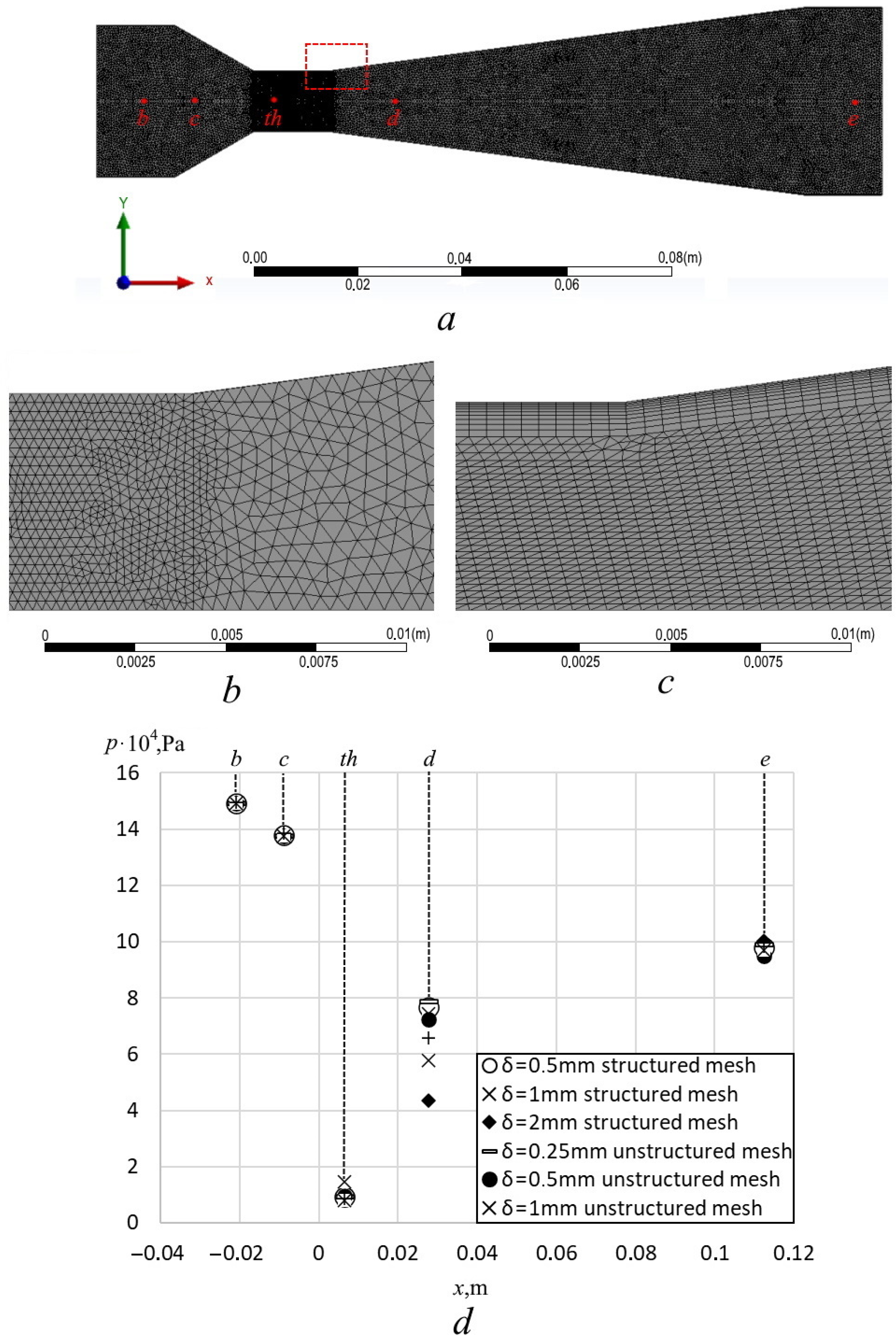
Mesh was refined as shown in Figure 4a. The cell size δ in the refinement region was four times smaller than in the other regions of the model. The magnified mesh region is shown in Figure 4b. A mesh study was conducted for the cell size and for the mesh structure. Structured mesh with the boundary layer region was also generated (Figure 4c). A total of 10 mesh layers were set near the wall with the maximum width of 1 mm. For this analysis, the mesh size was doubled every iteration (Figure 4d). The pressure at four characteristic points, which we used for cavitation number calculations (Figure 3), were used for comparison. Computational results demonstrated that the pressure in points “b”, “c” and “e” did not depend on size and type of the mesh. Some spread of the results was observed in the points “th” and “d” (Figure 4d). To stabilize results at these points the mesh size was reduced to δ < 0.5 mm for unstructured mesh and δ < 1 mm for structured mesh. On average, the computational grid consisted of 0.5 million elements.

4. Results and Discussion

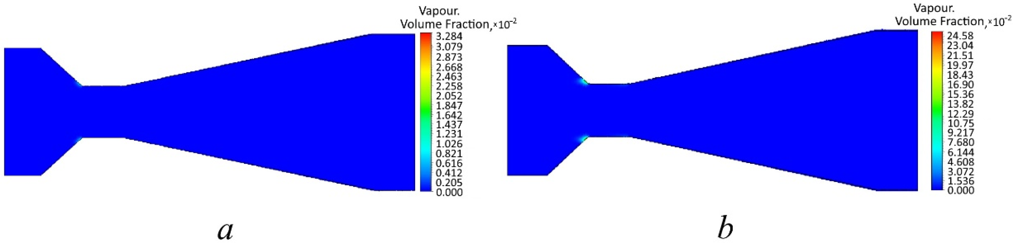
Validation of CFD results for the Venturi tube is shown in Figure 5. Cavitation occurs at the leading edge of the Venturi neck, at the beginning of the cylindrical portion. At the absolute pressure on the inlet p_in = 1.3 atm, cavitation cavern propagates through the throat of the Venturi tube (Figure 5a). The length of the cavitation region in this case was l_cavi = 18 mm. The increase of the inlet pressure to 1.5 atm leads to the appearance of cavitation bubbles along the entire surface of the neck and at the entrance to the Venturi diffuser. In this case, the length of the cavitation region increased to 26 mm (Figure 5c). CFD predictions showed a good agreement with the experimental results (Figure 5b,c). The back pressure (outlet) is 1 atm absolute. Therefore, when cavitation occurs for tap water with a temperature of 15 °C, the critical pressure difference inside the Venturi tube, determined experimentally, is 0.3 atm. The volume fraction of the vapor phase reaches 37%, and with a difference of 0.5 atm—48%.

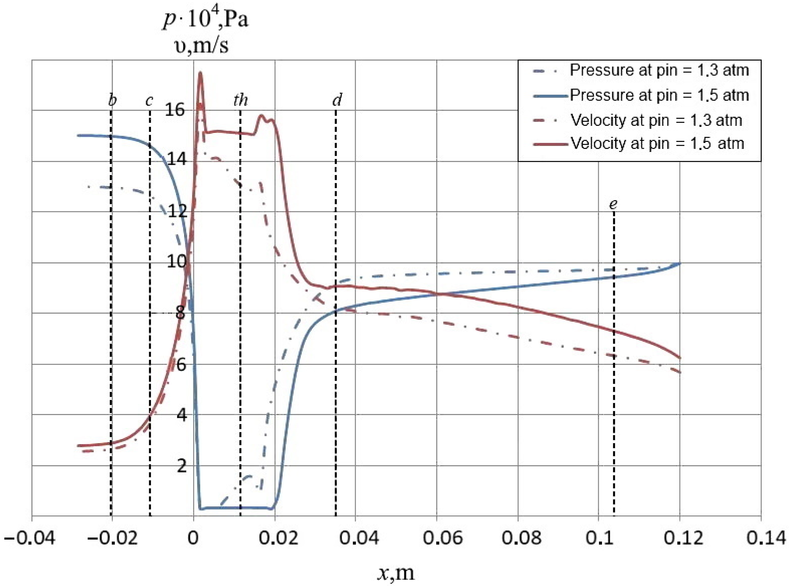
Figure 6 shows absolute pressure (blue line) and the flow velocity υ (red line) along the Venturi tube. Pressure (p_abs) decreases to the value of saturated vapor pressure p_v at x = 0, which corresponds to the beginning of the cylindrical section (throat) in the Venturi tube. At inlet pressure p_in = 1.3 atm, the length of the region near the nozzle wall, where p_abs = p_v, is equal to 5–6 mm. The size of the cavity is determined by the distance that cavitation bubbles will overcome after the nucleation, growth and implosive collapse in the high-pressure zone. Therefore, visually and numerically, we can observe that cavitation zone propagates further than the region where p_abs = p_v. (Figure 5a,b).

When inlet pressure is increased to p_in = 1.5 atm cavitation zone is propagating further to diffuser (Figure 5c,d). Based on Figure 3 and Figure 6, four points were selected for calculations of p_abs, υ and σ. Results for the calculated cavitation number σ are shown in

Table 1. Absolute pressure and velocity (in atm. and m/s) (from our CFD results).

Nozzle and Flow Direction	pa	pb	pc	pd	pe	υth	υb	υc	υd	υe
Venturi, straight	1.50	1.50	1.43	0.68	0.96	15.20	2.85	4.49	9.49	6.85
Venturi, straight	1.30	1.30	1.24	0.80	0.98	14.10	2.64	4.17	9.03	6.07
Venturi, reverse	1.50	1.50	1.02	0.90	0.88	14.30	1.77	9.93	10.10	9.51
Venturi, reverse	1.30	1.30	0.96	0.95	0.94	12.04	1.59	8.40	8.20	7.77
Venturi, reverse	1.65	1.65	1.08	0.87	0.82	15.57	1.94	10.85	11.19	10.48
Cylindrical	2.50	2.50	2.42	0.77	0.74	9.8	3.34	5.03	4.51	8.18
Cylindrical	2.80	2.80	2.72	0.70	0.66	10.34	3.50	5.27	3.22	8.74
Conical divergent	1.80	1.80	1.76	0.84	0.89	7.33	2.50	3.63	4.56	5.36
Conical divergent	1.80	1.74	1.60	0.67	0.70	13.72	4.18	6.79	9.14	10.05
Conic convergent	2.80	2.66	2.34	0.26	0.53	20.70	6.27	10.18	13.80	15.13

and

Table 2. Cavitation number (from our CFD results).

Nozzle and Flow Direction	σpa,υth	σpb,υth	σpb,υb	σpc,υth	σpc,υc	σpd,υth	σpd,υd	σpe,υth	σpe,υe
Venturi, straight	1.27	1.27	36.08	1.21	13.91	0.56	1.44	0.80	3.96
Venturi, straight	1.28	1.27	36.33	1.22	13.93	0.77	1.88	0.95	5.14
Venturi, reverse	1.44	1.44	93.73	0.97	2.00	0.85	1.71	0.82	1.86
Venturi, reverse	1.75	1.75	100.01	1.28	2.63	1.26	2.73	1.25	3.00
Venturi, reverse	1.33	1.33	85.88	0.87	1.79	0.69	1.34	0.65	1.44
Cylindrical	5.11	5.11	44.28	4.95	18.89	1.52	7.23	1.46	2.11
Cylindrical	5.18	5.18	45.10	5.02	19.34	1.25	12.89	1.18	1.65
Conical divergent	6.59	6.59	56.67	6.45	26.32	3.02	7.80	3.20	5.98
Conic convergent	1.88	1.81	19.58	1.66	6.78	0.68	1.54	0.71	1.33
Conic convergent	1.29	1.23	13.38	1.08	4.45	0.11	0.24	0.23	0.44

.

One of the disadvantages of the cavitation number is that it does not consider geometry of cavitation chamber. It can be demonstrated by changing the direction of the flow inside Venturi tube. Parameters for cavitation inception and cavitation zone size are shown in Figure 7. Characteristic points which were defined in Figure 3 are positioned in the opposite direction.

For the reversed flow in the Venturi tube, we did not observe cavitation at the inlet pressure p_in = 1.3 atm and 1.5 atm. We could observe cavitation inception at inlet pressure of 1.65 atm with a maximum vapor concentration 24% (Figure 8).

It can be seen, that for a Venturi tube flow the critical pressure drop for cavitation inception is 0.3 atm, and for the reversed flow with the same geometry it increases to 0.65 atm.

For the cylindrical nozzle (Figure 3b), cavitation inception could be observed at p_in = 2.5 atm. Figure 9 shows absolute pressure (blue line) and the flow velocity υ (red line) along the cylindrical nozzle including the case with switched inlet. For this type of nozzle, the critical pressure difference for cavitation inception was 1.5 atm.

Cavitation appears in the transition from wide to narrow section in the direction of flow. The length of cavitation region in this case was l_cavi = 10 mm The maximum vapor concentration is 80% (Figure 10a,b). When inlet pressure was increased to 2.8 atm, the entire throat was filled with vapor (l_cavi = 32 mm). The cavitation zone significantly increases but maximum volume fraction stays the same (Figure 10c,d).

Inception cavitation number for the case of cylindrical nozzle is significantly higher than in the case of Venturi tube in all characteristic points.

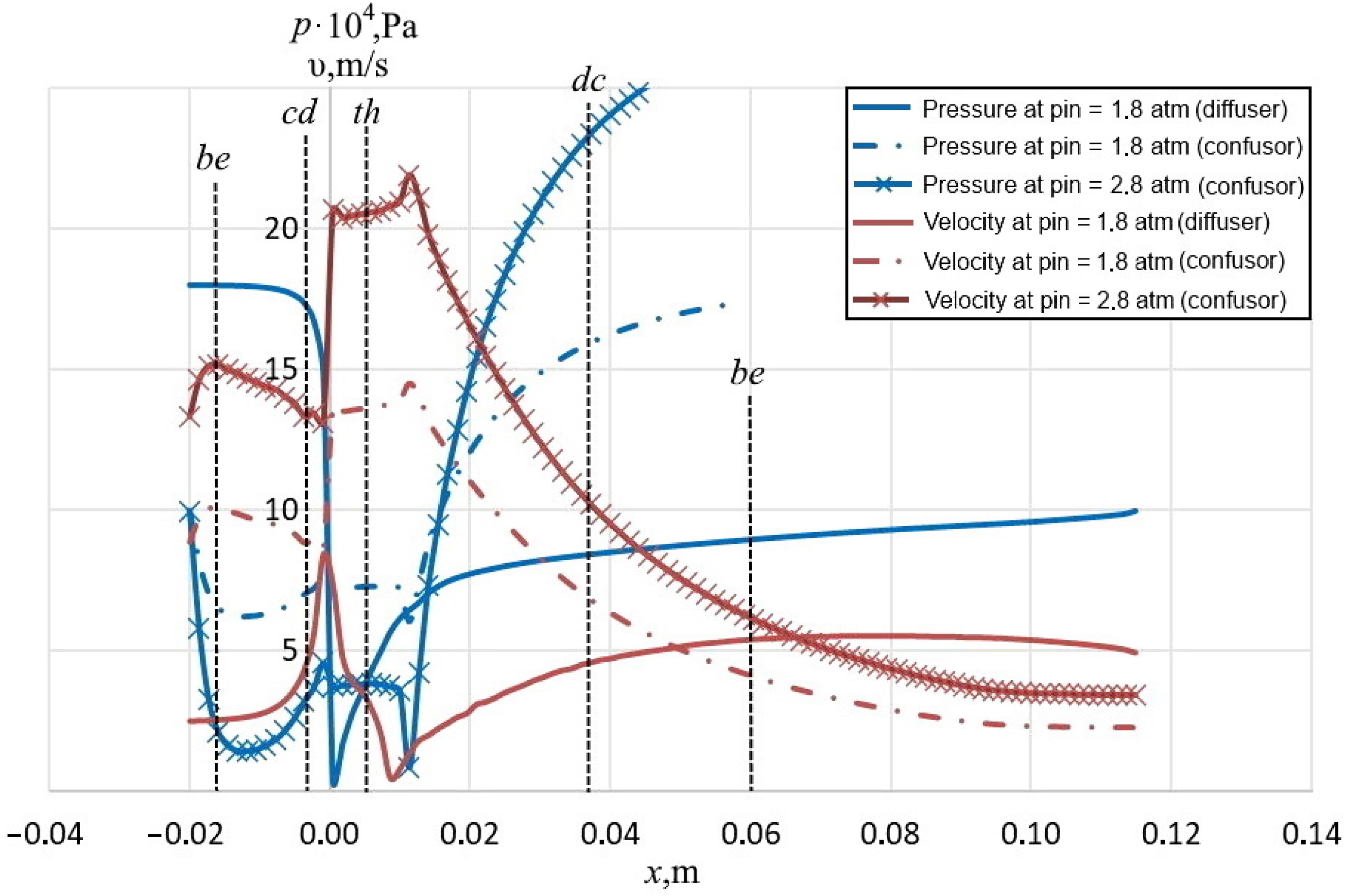
The last type of nozzle tested in this study was the convergent/divergent nozzle (Figure 3c). Figure 11 shows absolute pressure (blue line) and the flow velocity υ (red line) along the conical nozzle including the case with switched inlet. The characteristic points were determined when the cone acts as a diffuser or confuser for the fluid flow. For the smooth expansion of the flow (diffuser case), cavitation inception is observed at p_in = 1.35 atm and the cavity zone (l_cavi = 10 mm) gradually increases with increasing pressure (Figure 12). The critical pressure drop for cavitation inception was 0.35 atm. For the reversed case (converging nozzle) the phase transition starts only at p_in = 2.8 atm, and slowly increases with increasing pressure.

It can be seen that there is no pattern in changing of cavitation inception number for different geometries of the nozzles. Cavitation bubbles can appear at σ ≈ 1 and their quantity increases with a decrease in cavitation number. However, we can also observe the appearance of cavitation at σ = 5–6. From analysis of the cavitation number Formula (1), it can be noted that such a wide spread of cavitation numbers is related to velocity of the flow.

One of the most important parameters which affects cavitation inception and development is pressure difference between vapor pressure and local pressure which is reflected in cavitation number Formula (1).

The other parameter which affects cavitation development is fluid temperature. The temperature effect on cavitation was studied in [24,25,26,27]. It was shown that less cavitation bubbles were generated at low temperature (close to 0 °C for water) but the implosion of bubbles is much more intense. The quantity of cavitation bubbles grows with temperature increase, but the implosion energy decreases. The decrease in the implosion at elevated temperatures (close to 100 °C for water) occurs due to the bubbles’ inability to trap vapor, their volume grows and they consequently implode. An ideal balance between quantity of the cavitation bubbles and implosion power is achieved at 40–50 °C [6]. At different temperatures it is important to consider viscosity effect. Viscosity is decreasing at higher temperatures and Reynolds number is increasing. This effect is shown in CFD modelling in [28] and in experiments in [29]. Lower viscosity leads to increase of cavitation activity because of molecular connections weakening.

It should be noted that the temperature effect is usually considered for developed cavitation, when the cavitation zone reaches several centimeters in size. In this study, we considered the effect of temperature on the vapor fraction and cavitation zone length during the inception process. Vapor fraction n along the nozzle of Venturi tube type at different temperatures is shown in Figure 13. Inlet pressure in this case is 1.3 atm and corresponds to cavitation inception. The origin in Figure 13 corresponds to beginning of cylindrical throat. It can be seen that the length of cavitation zone is 27 mm and it is stable in the temperature range 25–75 °C. In the temperature range of 55–65 °C we can observe the appearance of a second local maximum of vapor fraction which corresponds to the transition to diffuser. Temperature increase to 75 °C leads to a significant increase of cavitation activity and increase of cavitation zone length (more than 30 mm (l_cavi > 30 mm)). The similar behavior of cavitation was observed at an increase of inlet pressure to 1.5 atm (Figure 5c,d).

The similar dependency of the vapor fraction from temperature for the conic nozzle (diverging) is shown in Figure 14. Inlet pressure in this case is 1.8 atm, which also corresponds to cavitation inception. The origin corresponds to transition to cylindrical part of the nozzle before the diffuser. The length of the cavitation zone does not exceed 10 mm in the temperature range from 25 to 75 °C, but the vapor fraction increases. The length of the cavitation zone and concentration of vapor are lower than in the case of the Venturi type of nozzle.

For the cylindrical nozzle, this relation of vapor fraction with temperature is qualitatively different (Figure 15). Inlet pressure in this case is 2.5 atm which corresponds to cavitation inception. The origin in Figure 15 corresponds to the transition to the throat. Temperature change in the range of 25–75 °C leads to an increase of cavitation region length without the changing of vapor fraction n. At 75 °C, the cavitation zone length reaches its maximum (40 mm).

In general, all physical values in Equation (1) have some relationship with temperature. The growth of vapor pressure p_v and decrease of density ρ of the fluid will lead to a change of pressure p_abs and velocity v in order for the cavitation number to reflect cavitation inception. This process is shown in Figure 16, Figure 17 and Figure 18 where we analyzed how temperature increase affects cavitation number. We can observe that the cavitation number decreases at the increase of temperature as well as the critical cavitation number which describes cavitation inception. 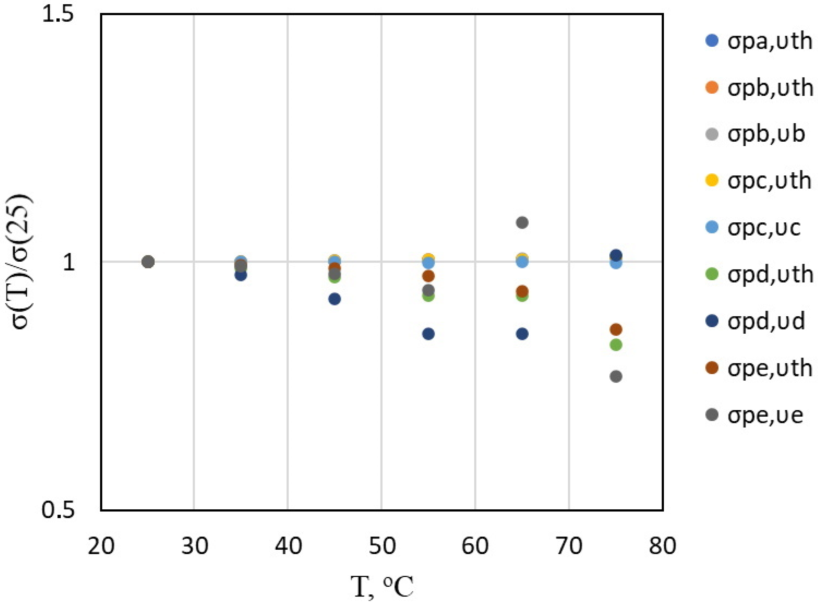For the Venturi tube type of nozzle (Figure 16) and conic nozzle (Figure 17), we have points where the cavitation number is constant for any temperatures in the range of 25–75 °C. For the conic nozzle (Figure 17) σ(25)/σ(T) has the maximum for characteristic point d in the cavitation nozzle after the cavitation zone. A further decrease of cavitation number is observed for pressure pe in the system after cavitation nozzle.

Table 1 shows the results of measurements of p_abs and υ, and Table 2 shows calculated cavitation number σ. As we can see, the cavitation number values are widespread depending on the method of their calculation. Cases with an absence of cavitation are marked and highlighted in bold.

5. Conclusions

The analysis of the flow velocity at the characteristic points did not reveal any obvious patterns. Based on this study, we can conclude that the smaller the σ, the closer we approach cavitation inception. It is necessary to choose the maximum velocity in cavitation number calculations. Using the velocity υ_th to calculate σ made it possible to reduce the spread of cavitation number values and only preserved the difference between the regions before and after the cavitation location. However, the use of υ_th for a cylindrical nozzle shows significantly overcalculated values of σ in comparison with other experiments and data from the literature.

Temperature dependency of cavitation inception and development is different for different types of nozzles. For Venturi tubes and conic nozzles, temperature increases lead to growth of the vapor fraction and for cylindrical nozzles lead to an increase of the cavitation zone.

In general, it can be concluded that the cavitation number calculation is clearly insufficient to predict cavitation inception and development in the fluid flow. In addition, this is likely not the main criterion that should be employed in engineering applications using hydrodynamic cavitation. The main disadvantage of σ is the absence in Equation (1) of a connection with the geometry of the cavitation nozzle, therefore, even if the input and output of the nozzle are reversed, this will not affect the calculations of σ in any way, but in fact it will have a significant impact on cavitation activity. Moreover, it should be noted that such parameters as temperature, scale factor, content of dissolved gases and quantity of mechanical particles in the flow must be considered for estimation of cavitation inception and development.