
Modeling of Flow Heat Transfer Processes and Aerodynamics in the Cabins of Vehicles


1
Department of Transport Systems, Faculty of Roads and Transport Systems, Don State Technical University, Gagarin, 1, 344003 Rostov-on-Don, Russia
2
Department of Theoretical and Applied Mechanics, Agribusiness Faculty, Don State Technical University, Gagarin, 1, 344003 Rostov-on-Don, Russia
3
Department of Life Safety and Environmental Protection, Faculty of Life Safety and Environmental Engineering, Don State Technical University, Gagarin, 1, 344003 Rostov-on-Don, Russia
*
Author to whom correspondence should be addressed.
Fluids 2022, 7(7), 226; https://doi.org/10.3390/fluids7070226
Submission received: 29 May 2022
/
Revised: 30 June 2022
/
Accepted: 1 July 2022
/
Published: 3 July 2022
Abstract
:Ensuring comfortable climatic conditions for operators in the cabin of technological machines is an important scientific and technical task affecting operator health. This article implements numerical and analytical modeling of the thermal state of the vehicle cabin, considering external airflow and internal ventilation. A method for calculating the heat transfer coefficients of a multilayer cabin wall for internal and external air under conditions of forced convective heat exchange is proposed. The cabin is located in the external aerodynamic flow to consider the speed and direction of the wind, as well as the speed of traffic. Inside the cabin, the operation of the climate system is modeled as an incoming flow of a given temperature and flow rate. The fields of velocities, pressures, and temperatures are calculated by the method of computer hydrodynamics for the averaged Navier–Stokes equations and the energy equation using the turbulence model. To verify the model, the values of the obtained heat transfer coefficients were compared with three applied theories obtained from experimental data based on dimensionless complexes for averaged velocities and calculated by a numerical method. It is shown that the use of numerical simulation considering the external air domain makes it possible to obtain more accurate results from 5% to 75% compared to applied theories, particularly in areas with large velocity gradients. This method makes it possible to get more accurate values of the heat transfer coefficients than for averaged velocities.
1. Introduction
Currently, the materials of the cabin of vehicles and mobile technological machines, including those for special purposes, are, as a rule, a complex multilayer composition of heat-insulating, decorative, protective, and other layers (Figure 1). Increasingly complex cabin materials, additional heat-loaded equipment, and increasing requirements for thermal comfort require the development of refined approaches to modeling the thermal state of vehicles. The creation of a microclimate in the cabin is the most important task to ensure optimal conditions for human HVAC (Heating, ventilation, air-conditioning) work, as well as for the operation of electronic equipment.
The factors that provide a comfortable microclimate and the theoretical foundations for modeling the microclimate in cabins based on the balance equations of heat flows are given in [1,2,3]. Heat transfer through the wall is modeled as convective heat exchange with the environment, which is characterized by heat transfer coefficients to the environment and the thermal conductivity of the wall [4,5,6,7,8,9,10].
Analytical determination of heat transfer coefficients relates to the solution of the system of Navier–Stokes equations. Hence, for free convection in a flat setting, methods for obtaining coefficients for flat horizontal and vertical plates and pipes were described [4,5,6,7,8,9,10].
In the general case of forced convection, due to the impossibility of obtaining an analytical solution of the Navier–Stokes equations, for such problems, the main way to find the heat transfer coefficients is the experiment and the Nusselt criterion based on dimensionless complexes and similarity theory [11,12,13,14,15,16], by averaging the temperature fields and speeds. The values of the heat transfer coefficients are found from the Nusselt number, which in turn depends on the nature of the medium flow in the near-wall regions. In practice, the applied formulas of Jürgens, Raman, and Frank [1,2,3] have become widely used.
Thus, experimental values were obtained, particularly for vertical and horizontal walls and pipes under natural and forced convection, for heat exchangers, taking into account the phase transitions of the liquid [17,18,19,20,21,22,23,24,25,26,27,28].
Computational fluid dynamics methods make it possible to obtain a numerical solution of hydrodynamic equations, considering complex boundary conditions. Modern research work is aimed at conducting virtual numerical tests, as well as finding and refining Nusselt values. Thus, in [29,30,31,32,33,34], the results of numerical studies and values of heat transfer coefficients for various tubular heat exchangers, in evaporators, coolers, and other surfaces are presented.
When modeling the problem of thermal comfort, determining the coefficient of convective heat transfer with internal and external air is one of the key tasks of heat and mass transfer and applied hydro aerodynamics, since the cabin geometry and the configuration of the climate system create a significantly uneven velocity field outside and inside the cabin.
In [35,36,37,38,39,40,41,42], the results of CFD analysis of thermal and hydrodynamic characteristics for various vehicles were presented, and optimization issues for various configurations and cab geometries were considered. Using numerical analysis based on CFD [43,44,45] makes it possible to obtain excellent results in modeling air flows, especially considering turbulence [46,47].
The review above shows that modeling of air flows in the cabins of technological machines is an important task. However, heat and mass transfer processes give good accuracy in the case of laminar flow and lead to large errors in turbulence. The primary aim of this work was to develop a numerical model of the air flow in the cabin of technological machines. The novelty of this work is in the development of a new model of aerodynamics inside the vehicle cabin based on the Navier–Stokes equations using turbulence models and energy equations and determining the cabin heat transfer coefficients, as well as comparison with applied theories, obtained through experimental data. The internal and external areas of air in the cabin are considered. Ansys Fluent is used as a numerical implementation of a CFD model. This method makes it possible to obtain the most accurate values of heat transfer coefficients and evaluate the applicability of applied theories, including those that depend on air velocities.
2. Materials and Methods
2.1. Problem Formulation
To describe the behavior of a compressible viscous gas medium, the Reynolds-averaged Navier–Stokes equations are used together with the continuity equation (RANS) in a 2D formulation [48,49,50,51,52].
Velocity, temperature, pressure, and density are used as the main variables: , .
The mechanical properties of a gas are described by the dynamic viscosity μ, thermal conductivity , and heat capacity , which are considered constant.
To close the system of equations of hydrodynamics, the Mendeleev–Clapeyron equation of state for an ideal gas is used, in which the variables pressure and density are related by the following formula:
where R is the universal gas constant, and M is the molar mass.
2.2. Boundary Conditions
As boundary conditions exist on the edge of the domain and the rigid body Ω, the no-slip conditions of the medium are set as follows:
where are the normal and tangential components of the velocity vector
Velocity values (profiles) are set at the input,
Pressure values are set at the outlet,
In a numerical implementation, the equation usually considers the pressure relative to the reference atmospheric pressure.
Since the moment equation contains second derivatives of velocities, it is necessary to set additional boundary conditions. Typically, such conditions are introduced at the exit as the value of certain velocities or derivatives of velocities equal to zero, which means the absence of velocities in some directions and the uniformity of velocities at the exit of their area.
For the energy equation at the boundary Ω, the values of temperatures or the values of heat fluxes are set as follows:
For the case of unsteady motion of the medium at the zero moment of time, the initial values of all fields are set.
Thus, the RANS system of equations, together with the boundary and initial conditions (Equations (2)–(5)) and the turbulence equations, forms a closed boundary value problem of differential equations regarding the averaged velocities , pressure p, and temperature T.
2.3. Convective Heat Transfer
In the case of convective heat exchange with the external region, the heat flux is set at the boundary as follows:
where is the heat transfer coefficient of the medium, and is the known external temperature.
In the case of convective heat transfer through a layered wall with the external environment, the heat transfer coefficient is calculated using the following formulas:
where R is the coefficient of thermal resistance, are the thickness and thermal conductivity of the i-th wall, and are the internal and external heat transfer coefficients of the medium.
In the general case, the heat transfer coefficients and the temperature field for the medium cannot be obtained analytically from the Navier–Stokes equations. For such problems, the primary way to find the heat transfer coefficients is through experiment and the Nusselt criterion based on dimensionless complexes and similarity theory [4,5,6,7,8,9,10,11,12,13,14,15,16].
where Nu is the Nusselt number, L is the characteristic size, and λ is the thermal conductivity.
For gases, the generalized equation of convective heat transfer has the following form:
where the Nusselt number is a function of the dimensionless Prandtl and Grashof numbers. The Prandtl and Grashof values, in turn, depend on the gas parameters, temperature, characteristic dimensions, and flow velocity.
Experimentally generalized equations of convective heat transfer were obtained for several cases. In particular, the formulas from [1,4,6,8,14] have become widely used. The following formulas are often used to calculate convective heat transfer in process transport cabins:
where is the air velocity along the wall.
Numerically, the heat transfer coefficients for cabin air and external space are determined from the value of the heat flux :
where are the heat flow from the wall in the direction of the outside air and the inner cabin, respectively, and are the external and internal temperatures.
The grid of finite volumes consisted of 32,518 tetrahedral cells with six fine wall layers. The mesh orthogonality parameter was 0.6, which, according to the Ansys documentation [43,48], is indicated as “normal quality”. Reducing the dimension of the elements did not lead to a significant difference in the results.
The numerical algorithm converged at 250 steps; an increase in the number of steps showed no difference in the results. The accuracy of the model was estimated from the difference in mass flow rates at the inlet and outlet in the external domain and cabin, which amounted to 0.002% and 1.5%, respectively.
3. Results
3.1. Numerical Analysis
RANS equations are solved numerically using turbulence models.
To date, many turbulence models are known, each of which shows sufficient accuracy in certain cases [48,49,50,51,52]. The most universal are the turbulence models [52], where the turbulence kinetic energy k and the kinetic energy dissipation rate ε in the first case and the turbulence kinetic energy k and the specific kinetic energy dissipation rate ω in the second case are assigned as additional unknowns.
Furthermore, all characteristics are considered averaged, and the bar is omitted from above.
In this paper, the boundary value problem was simulated numerically by the finite volume method in the Ansys Fluent software product. The turbulence model was used as the most versatile model [43,48,53,54,55,56].
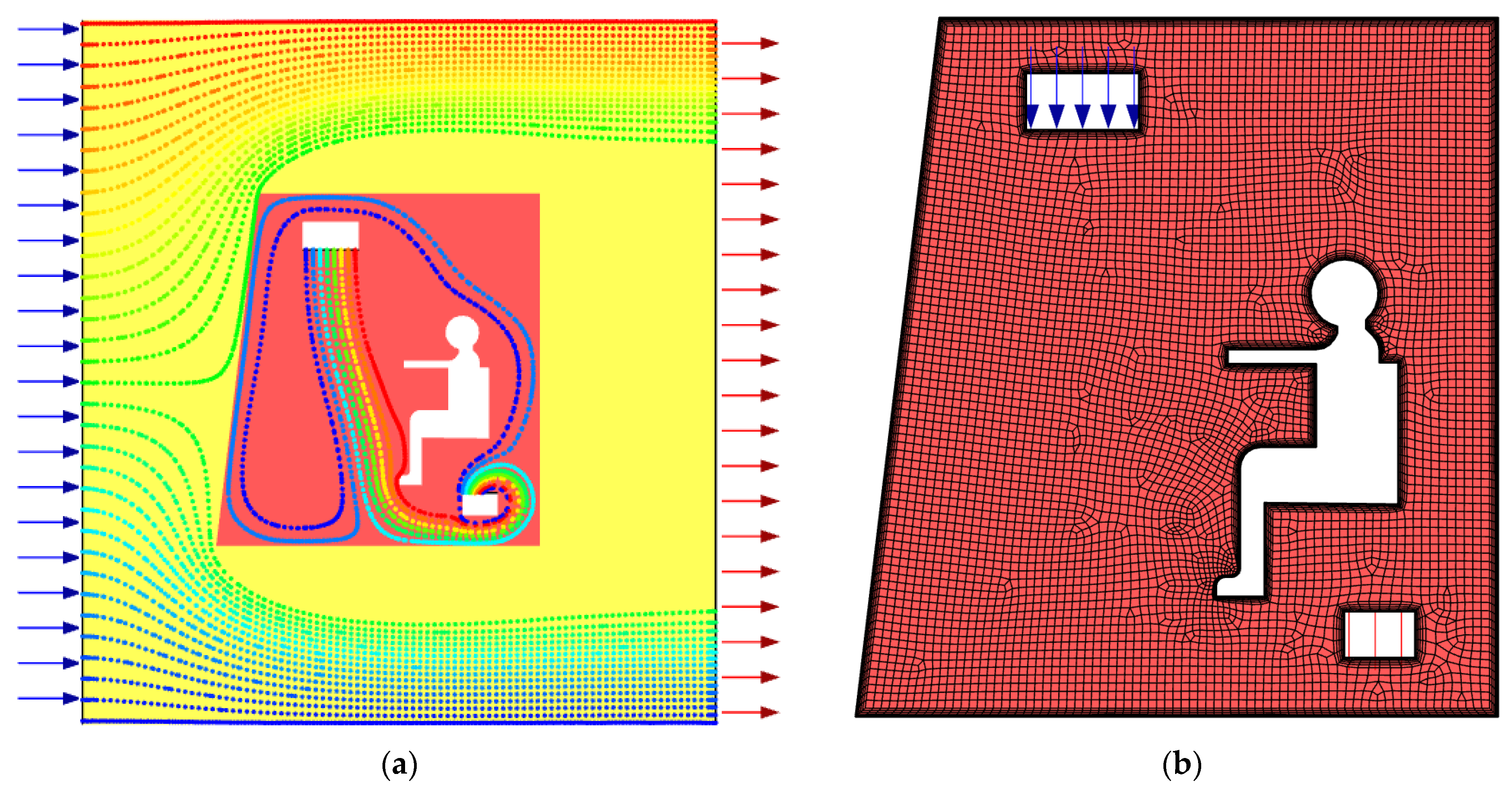
A rectangular cabin of technological transport in a wind tunnel is schematically shown in Figure 2a. Inside the cabin, there is a source through which air enters at a given speed and temperature. Zero relative pressure was set at the outlets. For clarity, all results are given for the middle section of the cabin for a flat formulation of the problem.
Figure 2b shows a finite volume grid of 32,518 cells with six near-wall layers to account for the gradient of edge effects.
The minimum cell area was 1.1 × 10⁻³ m2, and the maximum was 5.5 × 10⁻³ m2.
The grid orthogonality parameter was 0.6, which is quite acceptable for such problems [48].
3.2. Task Parameters
When modeling the problem of external aerodynamics, the size of the external domain depends significantly on the airflow velocities and the temperature gradient. In this problem, the external velocity was small, and the external temperature was constant along the entire domain outside the walls; therefore, the domain size was comparable to the cabin size, which made it possible to estimate the temperature and velocity fields near the walls.
The cabin wall (top, right) was a multilayer structure; according to Equations (7) and (8) and Table 1, the thermal conductivity coefficient for the walls was 0.33 W/(m∙K), and the thickness was 0.0312 m.
The left wall was made of laminated glass, with a thermal conductivity coefficient of 0.96 W/(m∙K). The bottom wall (floor) was thermally insulated.
Table 2 shows the values of the boundary conditions and air parameters.
3.3. Numerical Results
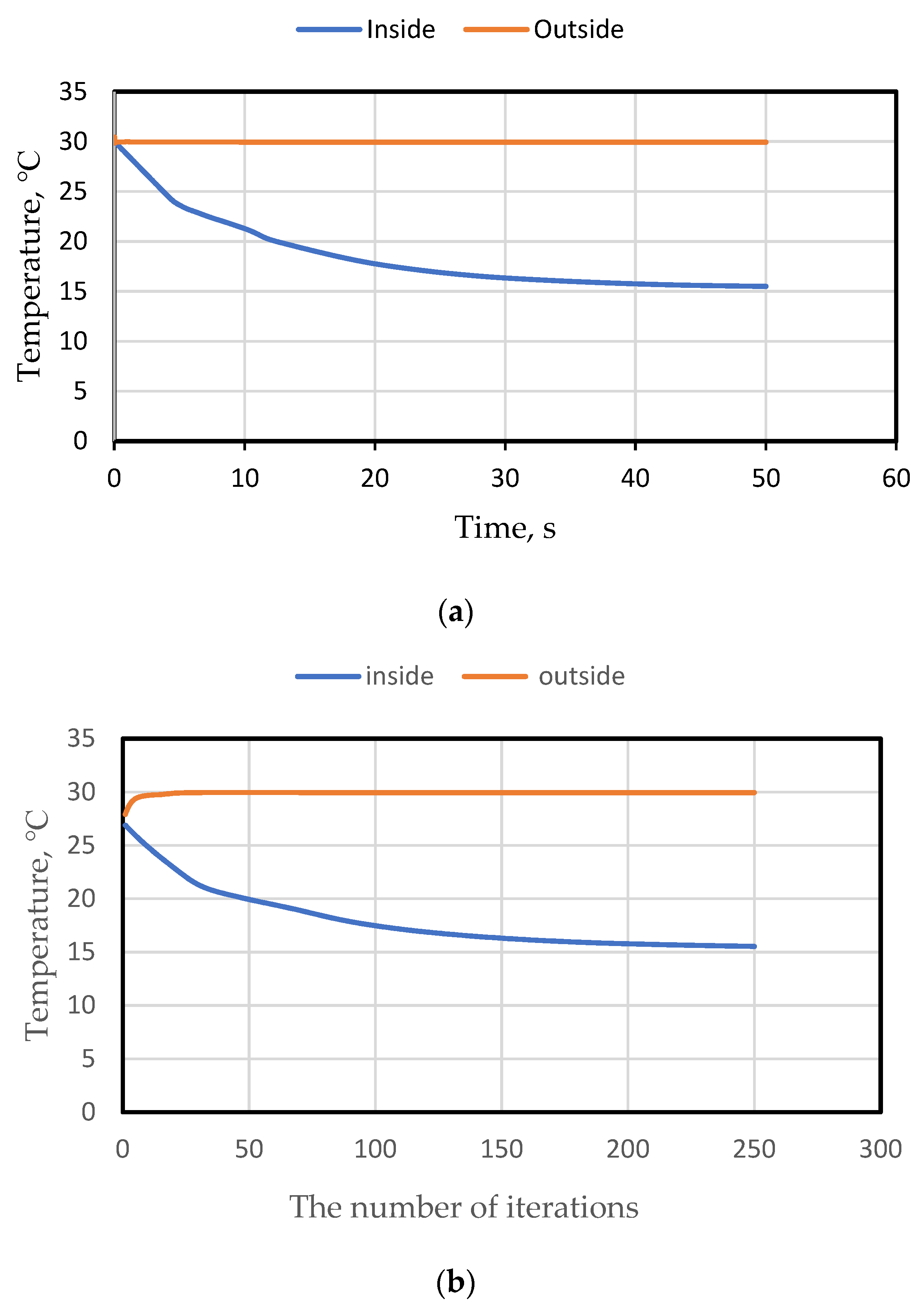
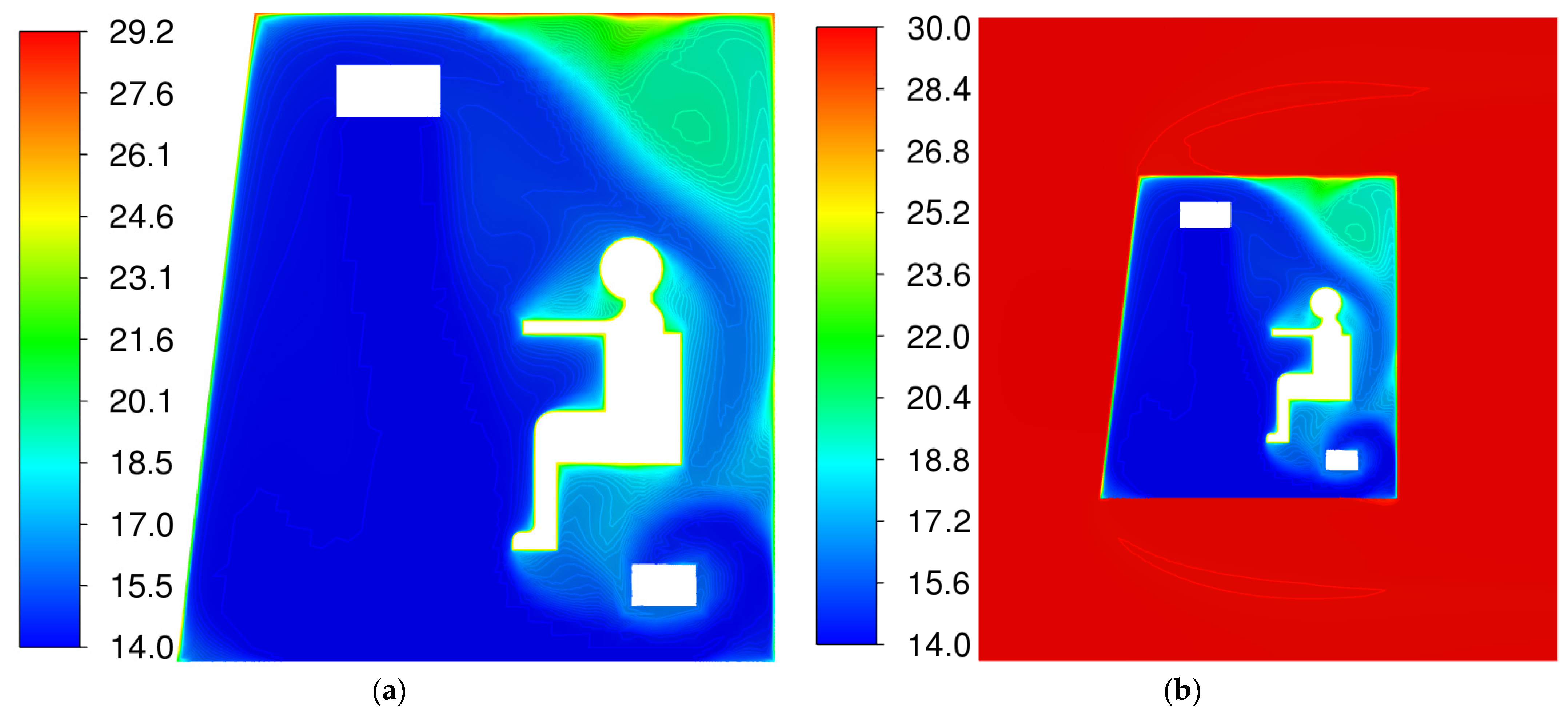
At the first stage, the nonstationary problem was solved. The initial temperature of the outer domain and inside the cabin was set to 30 °C. The stabilization time of the fields in time was 50 s (Figure 3a). Furthermore, all processes were stabilized in time, and the problem was solved in a stationary formulation.
Figure 3, Figure 4, Figure 5, Figure 6 and Figure 7 show plots of residuals, velocity fields, pressures, temperatures, and air densities.
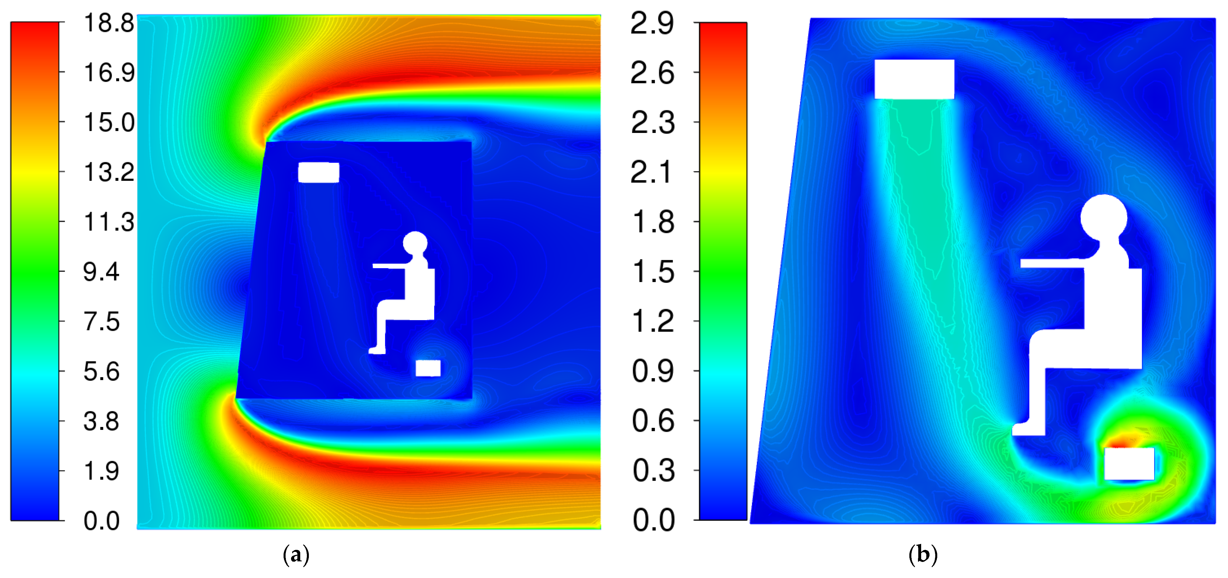
The average cabin temperature was 15.5 °C. The velocity and temperature fields inside the cabin turned out to be significantly inhomogeneous, characterized by streamlines (Figure 1a). The minimum air temperature was 14 °C in front of the driver, while the maximum air temperature above the walls was 29.2 °C. In addition, air stagnation could be observed in the upper right part.
In addition, the air flow and direction (and, therefore, temperature) were significantly affected by the interior layout of the cab space.
Numerical modeling in this case allows selecting the optimal combinations of the direction of air entering the cabin (configuration of deflectors), the number and location of deflectors, and the speed and temperature of the airflow.
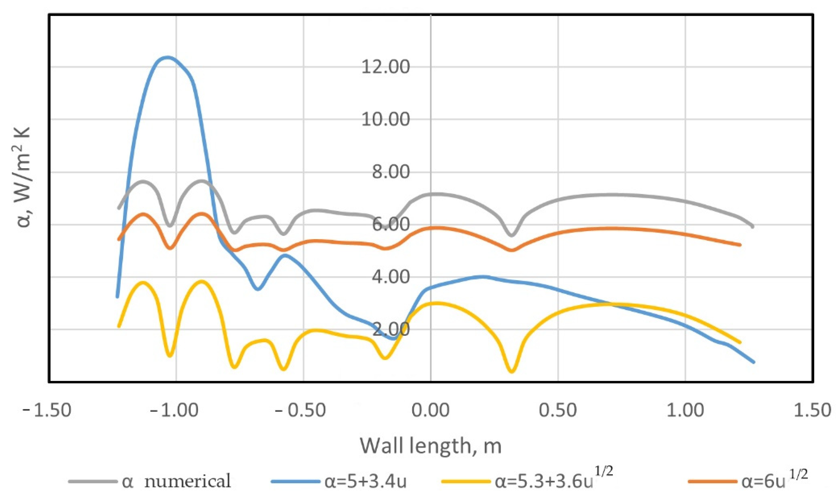
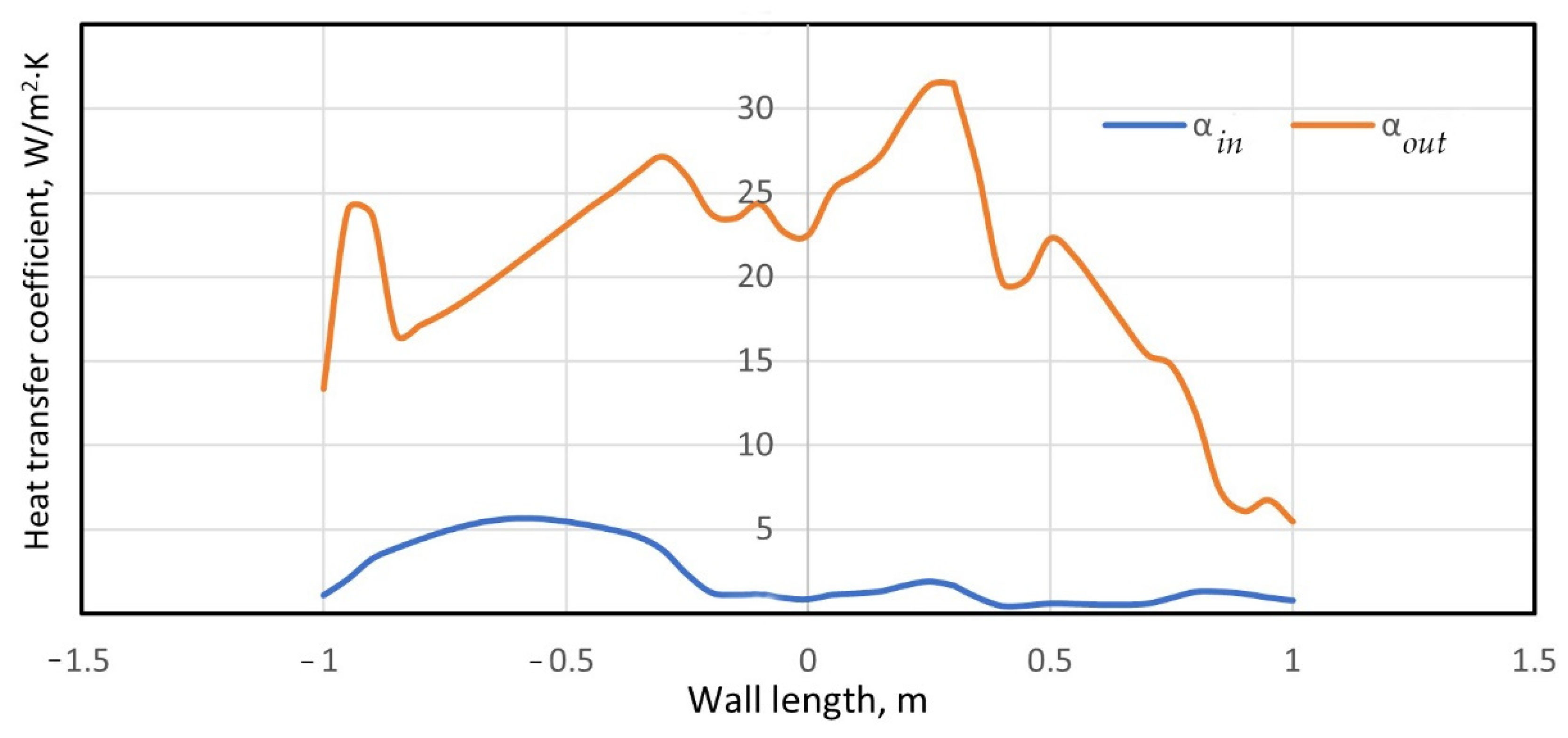
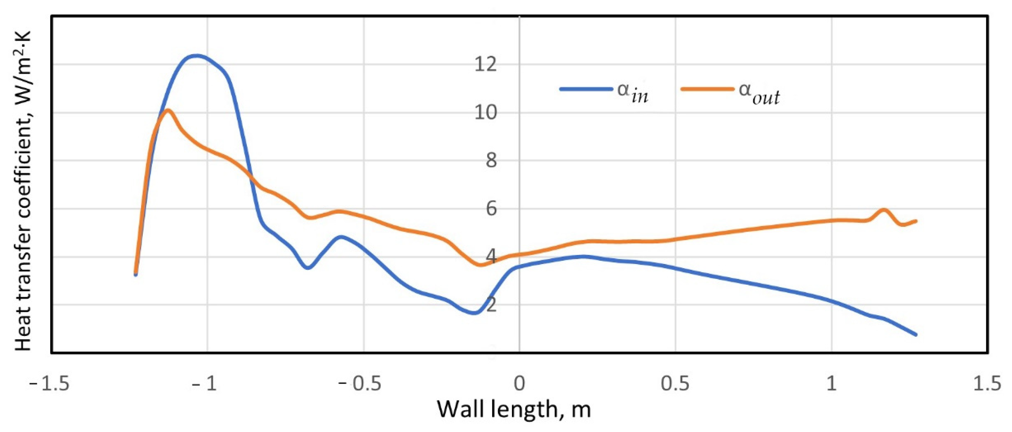
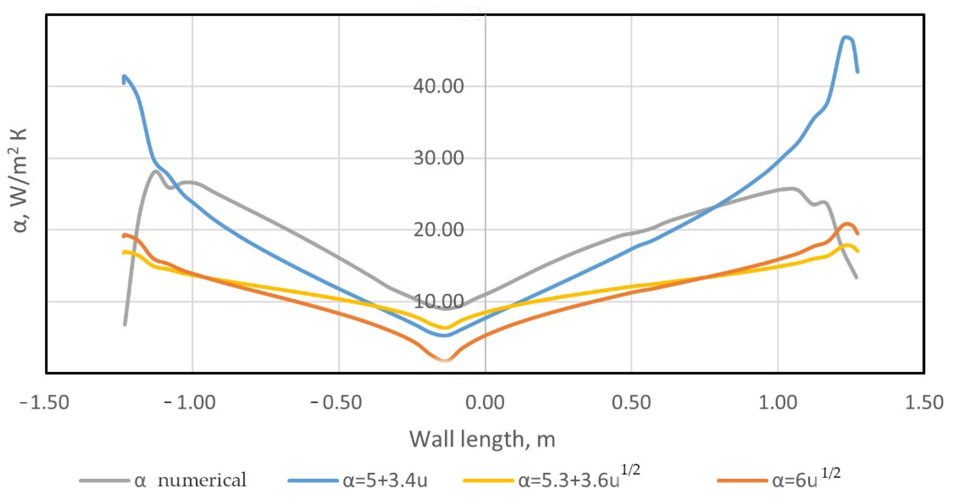
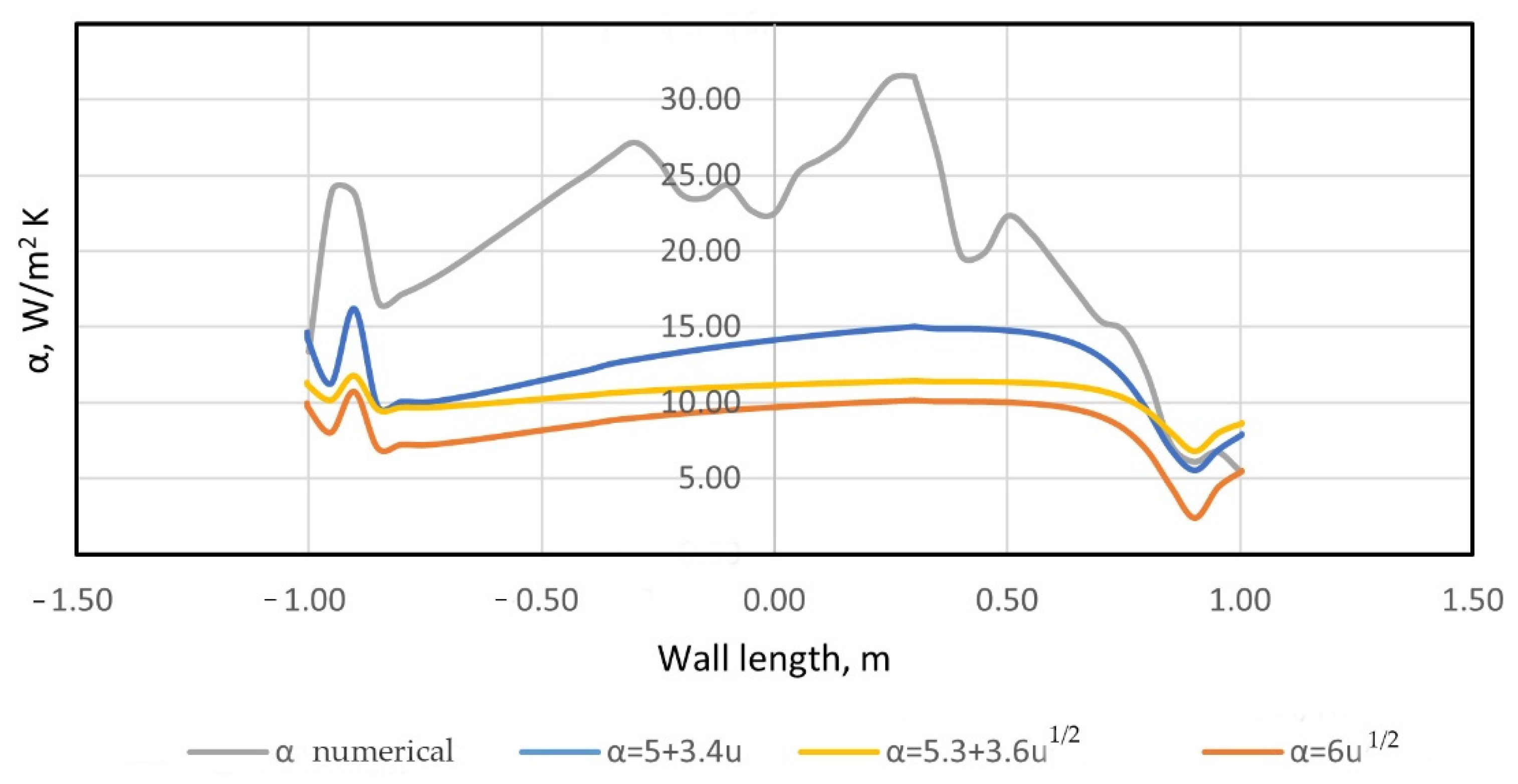
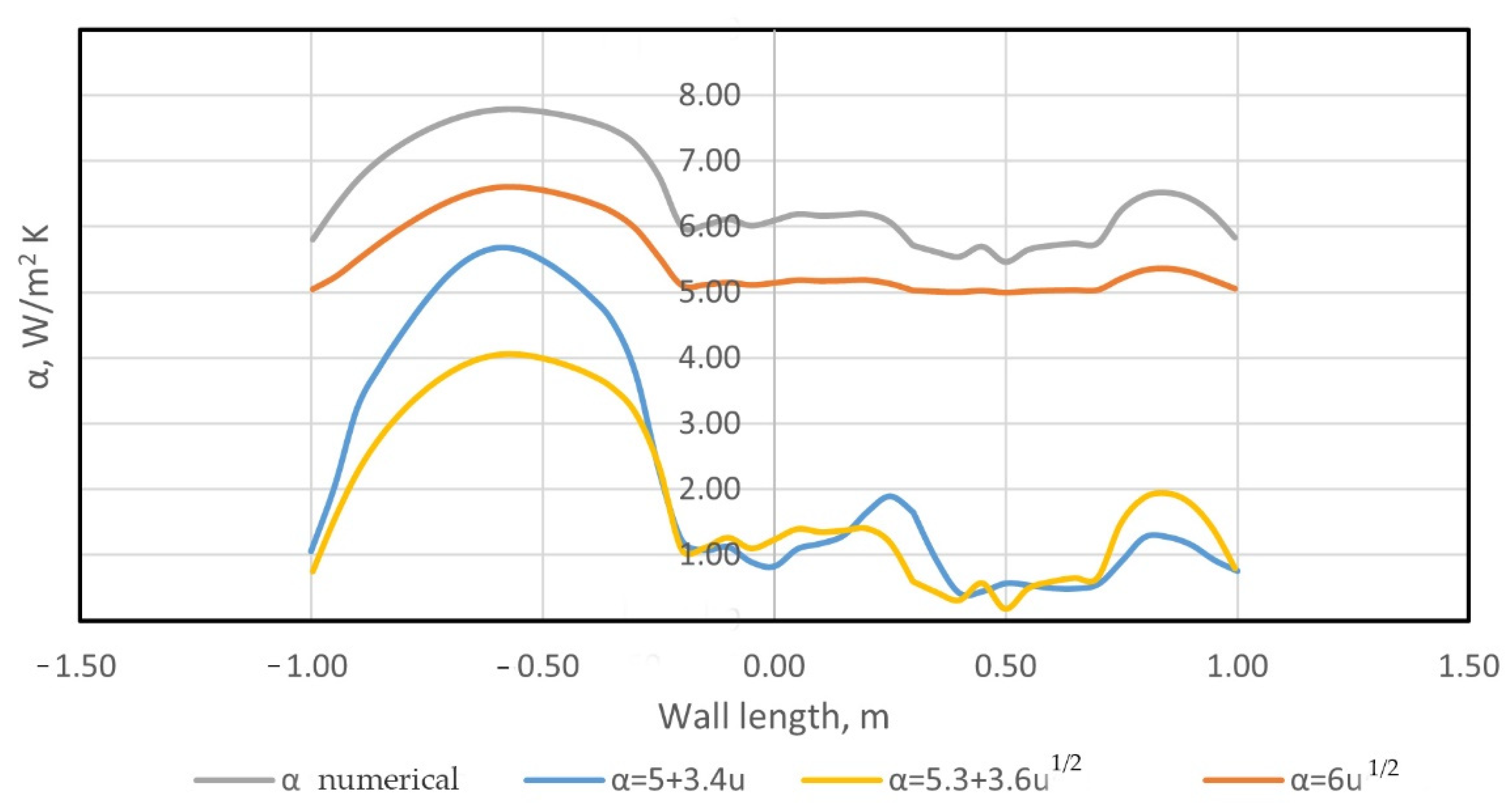
Figure 8, Figure 9, Figure 10, Figure 11, Figure 12 and Figure 13 show the values of heat transfer coefficients from Equations (14) and (15) and heat fluxes on the walls, obtained numerically.
It can be noted that the profiles of the heat transfer coefficients determined the air velocity profiles near the inner and outer walls, according to Equations (11)–(13). In particular, the values of the heat transfer coefficients had large gradients at the edges, where the velocity profiles changed direction.
4. Discussion
In the first case, the heat transfer coefficients calculated by applying Equations (11)–(13) and the average numerical values were compared. At the same time, for applied theories, the speed of the oncoming flow was taken as the speed of the external flow, and the average speed in the cabin, calculated from the balance equation, was taken as the internal one.
where G is the mass flow, and L is the width of the cabin along the vertical axis.
When ρ is constant inside the cabin, Equation (16) can be rewritten as
For an inlet speed of 1 m/s, , the average speed from Equation (17) in the cabin is 0.2 m/s.
Comparison data of heat transfer coefficients with formulas obtained on the basis of experimental data [1,4,6] are given in Table 3 and Table 4.
To verify the numerical model, we compared the results obtained with the experimentally obtained formulas used in practice (Table 3 and Table 4).
From Table 3 and Table 4, it can be seen that the smallest error in determining the thermal conductivity coefficient was achieved on the left wall and was best described by the formula . In this case, the error did not exceed 14% and could be explained using a 2D model for numerical calculation and the absence of internal equipment in the cabin.
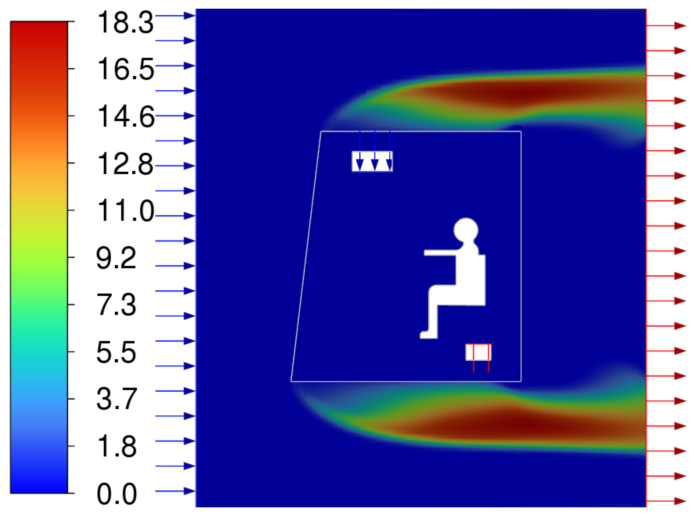
The large difference in the values of the coefficients in Table 3 can be explained by the nonuniformity of velocities along the walls, including turbulence zones over sharp edges (Figure 14). The obstacles inside the cabin in the form of equipment and controls can lead to even greater discrepancy in the results.
To study the influence of velocities, the values of velocities along the walls in the near-wall layer were additionally calculated for distances of one cell, which corresponds to 6 mm.
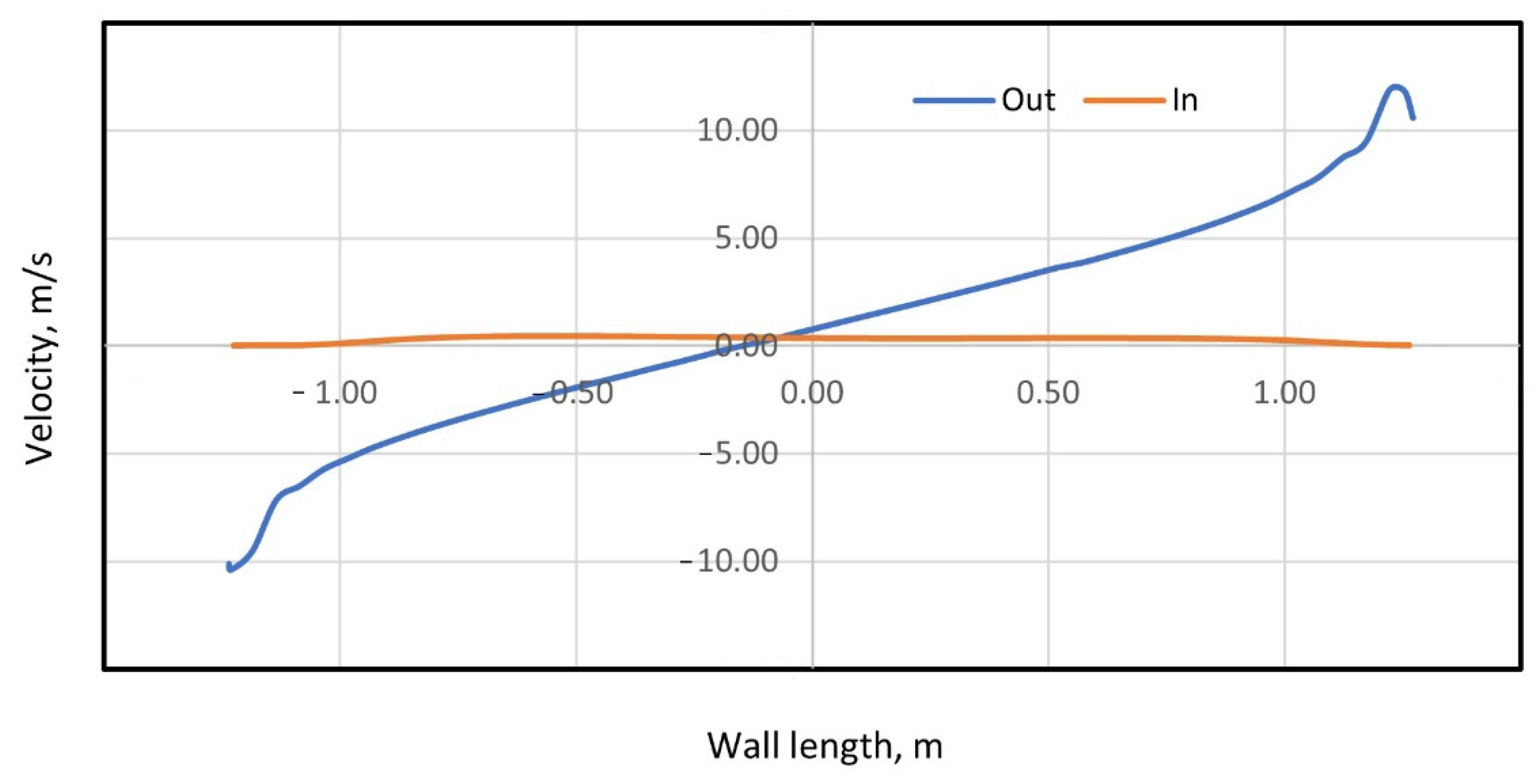
In the boundary value problem in Equation (2), all velocities on the walls were equal to zero, but they increased rather quickly when moving away from the walls. As an example, Figure 15 shows the velocity along the horizontal axis at a distance of three outer layers and three inner layers of the grid.
The points correspond to the values in the nodes. It can be seen that, at a distance of 6 mm, the speed increased and stabilized.
The speed values are shown in Figure 16, Figure 17 and Figure 18. Here, In denotes the speed inside the cabin, while Out denotes the speed outside the cabin.
5. Conclusions
In this study, numerical–analytical modeling of the thermal state of the vehicle cabin was carried out, considering external airflow and internal ventilation, the values of heat transfer coefficients for the walls were obtained, a comparison was made with existing empiric formulas based on experimental data, and an assessment was made of the applicability of applied theories.
- To calculate the values of the coefficients using applied formulas, the key point is the availability of sufficiently accurate values of the velocity profiles over the walls. Therefore, in this paper, it is shown that, when choosing the average internal and external speeds as the air speeds, the difference with the numerical results ranges from 5% to 75%. The reason for this error is the use of average velocities in the cabin and in the domain in applied theories, which does not correctly reflect the real velocity field.
- The problem of finding the values of the velocity fields is related to the solution of the Navier–Stokes equations and in most cases can only be solved numerically.
- In this work, we also compared the values of the heat transfer coefficients obtained by the numerical method and the values obtained from applied theories. The velocity fields in this case for applied theories were taken from a preliminary numerical calculation in near-wall regions.
- This approach can be applied to simulate the thermal state of cabins of any complexity, with high air flow rates and with various configurations of climate equipment inside the cabin. The proposed numerical implementation can be considered as the most optimal alternative for obtaining values on the basis of experimental data. Applied formulas give a significant error, since they do not consider the gradients of velocities and temperatures, and they can be used with certain restrictions.
- Validation was carried out to calculate the average temperature in the cabin of the technological transport in the absence of external airflow. The difference with the numerical model of the average temperature was about 9%.
Author Contributions
Conceptualization, I.P. and A.N.B.; methodology, I.P. and A.N.B.; software, I.P.; validation, I.P. and A.N.B.; formal analysis, I.P.; investigation, I.P., A.N.B. and B.M.; resources, B.M.; data curation, I.P.; writing—original draft preparation, I.P. and A.N.B.; writing—review and editing, I.P. and A.N.B.; visualization, I.P.; supervision, B.M.; project administration, B.M.; funding acquisition, A.N.B. and B.M. All authors have read and agreed to the published version of the manuscript.
Funding
This research received no external funding.
Institutional Review Board Statement
Not applicable.
Informed Consent Statement
Not applicable.
Data Availability Statement
The study did not report any data.
Acknowledgments
The authors would like to acknowledge the administration of Don State Technical University for their resources and financial support.
Conflicts of Interest
The authors declare no conflict of interest.
References
- Mikhailov, M.V.; Guseva, S.V. Microclimate in the Cabins of Mobile Vehicles; Engineering: Moscow, Russia, 1977; 230p. [Google Scholar]
- Panfilov, I.A.; Soloviev, A.N.; Matrosov, A.A.; Meskhi, B.C.; Polushkin, O.O.; Rudoy, D.V.; Pakhomov, V.I. Finite element simulation of airflow in a field cleaner. In Proceedings of the IOP Conference Series: Materials Science and Engineering, Rostov-on-Don, Russia, 20–22 October 2020; Volume 1001, p. 012060. [Google Scholar] [CrossRef]
- Meskhi, B.; Rudoy, D.; Lachuga, Y.; Pakhomov, V.; Soloviev, A.; Matrosov, A.; Panfilov, I.; Maltseva, T. Finite Element and Applied Models of the Stem with Spike Deformation. Agriculture 2021, 11, 1147. [Google Scholar] [CrossRef]
- Kirillin, V.A.; Sychev, V.V.; Sheindlin, A.E. Technical Thermodynamics; Energoatomizdat: Moscow, Russia, 1983; 416p. [Google Scholar]
- Beskopylny, A.; Kadomtseva, E.; Strelnikov, G. Numerical study of the stress-strain state of reinforced plate on an elastic foundation by the Bubnov-Galerkin method. In Proceedings of the IOP Conference Series: Earth and Environmental Science, Rostov-on-Don, Russia, 10–13 April 2017; Volume 90, p. 012017. [Google Scholar] [CrossRef]
- Andryushchenko, A.I. Fundamentals of Technical Thermodynamics of Real Processes; Higher School: Moscow, Russia, 1973; 264p. [Google Scholar]
- Baehr, H.D.; Kabelac, S. Thermodynamik; Springer: Berlin/Heidelberg, Germany, 2012; 667p. [Google Scholar] [CrossRef]
- Bazarov, I.P. Thermodynamics; Higher School: Moscow, Russia, 1983; 341p. [Google Scholar]
- Beskopylny, A.; Chukarin, A.; Meskhi, B.; Isaev, A. Modeling of Vibroacoustic Characteristics of Plate Structures of Vehicles during Abrasive Processing. Transp. Res. Procedia 2021, 54, 39–46. [Google Scholar] [CrossRef]
- Soloviev, A.N.; Oganesyan, P.A.; Skaliukh, A.S.; Duong, L.V.; Gupta, V.K.; Panfilov, I.A. Comparison between applied theory and final element method for energy harvesting non-homogeneous piezoelements modeling. Springer Proc. Phys. 2017, 193, 473–484. [Google Scholar] [CrossRef]
- Kuzovlev, V.A. Technical Thermodynamics and Basics of Heat Transfer, 2nd ed.; Higher School: Moscow, Russia, 1983; 335p. [Google Scholar]
- Kutateladze, S.S. Heat Transfer and Hydrodynamic Resistance: A Reference Guide; Energoatomizdat: Moscow, Russia, 1990; 367p. [Google Scholar]
- Beskopylny, A.N.; Kadomtseva, E.E.; Strelnikov, G.P.; Berdnik, Y.A. Stress-strain state of reinforced bimodulus beam on an elastic foundation. In Proceedings of the IOP Conference Series: Earth and Environmental Science, Rostov-on-Don, Russia, 10–13 April 2017; Volume 90, p. 012064. [Google Scholar] [CrossRef] [Green Version]
- Mikheev, M.A.; Mikheeva, I.M. Fundamentals of Heat Transfer, 2nd ed.; Energy: Moscow, Russia, 1977; 344p. [Google Scholar]
- Panfilov, I.A.; Ustinov, Y.A. Harmonic vibrations and waves in a cylindrical helically anisotropic shell. Mech. Solids 2012, 47, 195–204. [Google Scholar] [CrossRef]
- Kreith, F.; Black, W.Z. Basic Heat Transfer; Harper and Row: New York, NY, USA, 1980; 512p. [Google Scholar]
- Bruno, R.; Ferraro, V.; Bevilacqua, P.; Arcuri, N. On the assessment of the heat transfer coefficients on building components: A comparison between modeled and experimental data. Build. Environ. 2022, 216, 108995. [Google Scholar] [CrossRef]
- Liu, S.; Mu, X.; Shen, S.; Li, C.; Wang, B. Experimental study on the distribution of local heat transfer coefficient of falling film heat transfer outside horizontal tube. Int. J. Heat Mass Transf. 2021, 170, 121031. [Google Scholar] [CrossRef]
- Ibrahim, R.A.; Tittelein, P.; Lassue, S.; Chehade, F.H.; Zalewski, L. New Supply-Air Solar Wall with Thermal Storage Designed to Preheat Fresh Air: Development of a Numerical Model Adapted to Building Energy Simulation. Appl. Sci. 2022, 12, 3986. [Google Scholar] [CrossRef]
- Bilawane, R.R.; Mandavgade, N.K.; Kalbande, V.N.; Patle, L.J.; Kanojiya, M.T.; Khorgade, R.D. Experimental investigation of natural convection heat transfer coefficient for roughed inclined plate. Mater. Today Proc. 2021, 46, 7926–7931. [Google Scholar] [CrossRef]
- Che, M.; Elbel, S. Experimental quantification of air-side row-by-row heat transfer coefficients on fin-and-tube heat exchangers. Int. J. Refrig. 2021, 131, 657–665. [Google Scholar] [CrossRef]
- Moghadam, M.T.; Behabadi, M.A.A.; Sajadi, B.; Razi, P.; Zakaria, M.I. Experimental study of heat transfer coefficient, pressure drop and flow pattern of R1234yf condensing flow in inclined plain tubes. Int. J. Heat Mass Transf. 2020, 160, 120199. [Google Scholar] [CrossRef]
- Zakeralhoseini, S.; Sajadi, B.; Akhavan Behabadi, M.A.; Azarhazin, S.; Fazelnia, H. Experimental investigation of the heat transfer coefficient and pressure drop of R1234yf during flow condensation in helically coiled tubes. Int. J. Therm. Sci. 2020, 157, 106516. [Google Scholar] [CrossRef]
- Zhang, Y.; Cao, Y.; Gong, K.; Liu, S.; Wang, L.; Chen, Z. Numerical Study on Flow and Heat Transfer of Supercritical Hydrocarbon Fuel in Curved Cooling Channel. Appl. Sci. 2022, 12, 2356. [Google Scholar] [CrossRef]
- Lyapin, A.; Beskopylny, A.; Meskhi, B. Structural Monitoring of Underground Structures in Multi-Layer Media by Dynamic Methods. Sensors 2020, 20, 5241. [Google Scholar] [CrossRef] [PubMed]
- Jakubowska, B.; Mikielewicz, D.; Klugmann, M. Experimental study and comparison with predictive methods for flow boiling heat transfer coefficient of HFE7000. Int. J. Heat Mass Transf. 2019, 142, 118307. [Google Scholar] [CrossRef]
- Ammar, S.M.; Abbas, N.; Abbas, S.; Ali, H.M.; Hussain, I.; Janjua, M.M.; Dahiya, A. Condensing heat transfer coefficients of R134a in smooth and grooved multiport flat tubes of automotive heat exchanger: An experimental investigation. Int. J. Heat Mass Transf. 2019, 134, 366–376. [Google Scholar] [CrossRef]
- Che, M.; Elbel, S. An experimental method to quantify local air-side heat transfer coefficient through mass transfer measurements utilizing color change coatings. Int. J. Heat Mass Transf. 2019, 144, 118624. [Google Scholar] [CrossRef]
- Santosa, I.M.C.; Tsamos, K.M.; Gowreesunker, B.L.; Tassou, S.A. Experimental and CFD investigation of overall heat transfer coefficient of finned tube CO2 gas coolers. Energy Procedia 2019, 161, 300–308. [Google Scholar] [CrossRef]
- Wan, Y.; Soh, A.; Shao, Y.; Cui, X.; Tang, Y.; Chua, K.J. Numerical study and correlations for heat and mass transfer coefficients in indirect evaporative coolers with condensation based on orthogonal test and CFD approach. Int. J. Heat Mass Transf. 2020, 153, 119580. [Google Scholar] [CrossRef]
- Gao, S.; Ooka, R.; Oh, W. Formulation of human body heat transfer coefficient under various ambient temperature, air speed and direction based on experiments and CFD. Build. Environ. 2019, 160, 106168. [Google Scholar] [CrossRef]
- Liu, X.; Deen, N.G.; Tang, Y. On the treatment of bed-to-wall heat transfer in CFD-DEM simulations of gas-fluidized beds. Chem. Eng. Sci. 2021, 236, 116492. [Google Scholar] [CrossRef]
- Teodosio, L.; Timpone, F.; Napolitano dell’Annunziata, G.; Genovese, A. RANS 3D CFD simulations to enhance the thermal prediction of tyre thermodynamic model: A hierarchical approach. Results Eng. 2021, 12, 100288. [Google Scholar] [CrossRef]
- Song, H.; Fan, S.; Qu, D. Experimental Study on Flow and Heat Transfer Characteristics in the Circular-Arc-Shaped Flow Channel. Appl. Sci. 2022, 12, 376. [Google Scholar] [CrossRef]
- Karthick, L.; Prabhu, D.; Rameshkumar, K.; Prabhu, T.; Jagadish, C.A. CFD analysis of rotating diffuser in a SUV vehicle for improving thermal comfort. Mater. Today Proc. 2022, 52, 1014–1025. [Google Scholar] [CrossRef]
- Hemmati, S.; Doshi, N.; Hanover, D.; Morgan, C.; Shahbakhti, M. Integrated cabin heating and powertrain thermal energy management for a connected hybrid electric vehicle. Appl. Energy 2021, 283, 116353. [Google Scholar] [CrossRef]
- Bandi, P.; Manelil, N.P.; Maiya, M.P.; Tiwari, S.; Thangamani, A.; Tamalapakula, J.L. Influence of flow and thermal characteristics on thermal comfort inside an automobile cabin under the effect of solar radiation. Appl. Therm. Eng. 2022, 203, 117946. [Google Scholar] [CrossRef]
- Tan, L.; Yuan, Y. Computational fluid dynamics simulation and performance optimization of an electrical vehicle Air-conditioning system. Alex. Eng. J. 2022, 61, 315–328. [Google Scholar] [CrossRef]
- Singh, S.; Abbassi, H. 1D/3D transient HVAC thermal modeling of an off-highway machinery cabin using CFD-ANN hybrid method. Appl. Therm. Eng. 2018, 135, 406–417. [Google Scholar] [CrossRef]
- Chang, T.-B.; Sheu, J.-J.; Huang, J.-W.; Lin, Y.-S.; Chang, C.-C. Development of a CFD model for simulating vehicle cabin indoor air quality. Transp. Res. Part D Transp. Environ. 2018, 62, 433–440. [Google Scholar] [CrossRef]
- Ahmed Mboreha, C.; Jianhong, S.; Yan, W.; Zhi, S.; Yantai, Z. Investigation of thermal comfort on innovative personalized ventilation systems for aircraft cabins: A numerical study with computational fluid dynamics. Therm. Sci. Eng. Prog. 2021, 26, 101081. [Google Scholar] [CrossRef]
- Oh, J.; Choi, K.; Son, G.; Park, Y.-J.; Kang, Y.-S.; Kim, Y.-J. Flow analysis inside tractor cabin for determining air conditioner vent location. Comput. Electron. Agric. 2020, 169, 105199. [Google Scholar] [CrossRef]
- Kaewbumrung, M.; Charoenloedmongkhon, A. Numerical Simulation of Turbulent Flow in Eccentric Co-Rotating Heat Transfer. Fluids 2022, 7, 131. [Google Scholar] [CrossRef]
- Abdel Aziz, S.S.; Saber Salem Said, A.-H. Numerical Investigation of Flow and Heat Transfer over a Shallow Cavity: Effect of Cavity Height Ratio. Fluids 2021, 6, 244. [Google Scholar] [CrossRef]
- Lahaye, D.; Nakate, P.; Vuik, K.; Juretić, F.; Talice, M. Modeling Conjugate Heat Transfer in an Anode Baking Furnace Using OpenFoam. Fluids 2022, 7, 124. [Google Scholar] [CrossRef]
- Lv, X.; Wu, W.-T.; Lv, J.; Mao, K.; Gao, L.; Li, Y. Study on the Law of Pseudo-Cavitation on Superhydrophobic Surface in Turbulent Flow Field of Backward-Facing Step. Fluids 2021, 6, 200. [Google Scholar] [CrossRef]
- Vlasov, M.N.; Merinov, I.G. Application of an Integral Turbulence Model to Close the Model of an Anisotropic Porous Body as Applied to Rod Structures. Fluids 2022, 7, 77. [Google Scholar] [CrossRef]
- Fluent User’s Guide: Release 2022 R1 January 2022; ANSYS Inc.: Canonsburg, PA, USA, 2022; Available online: http://www.pmt.usp.br/academic/martoran/notasmodelosgrad/ANSYS%20Fluent%20Users%20Guide.pdf (accessed on 28 May 2022).
- Couto, N.; Bergada, J.M. Aerodynamic Efficiency Improvement on a NACA-8412 Airfoil via Active Flow Control Implementation. Appl. Sci. 2022, 12, 4269. [Google Scholar] [CrossRef]
- Klein, M.; Trummler, T.; Urban, N.; Chakraborty, N. Multiscale Analysis of Anisotropy of Reynolds Stresses, Subgrid Stresses and Dissipation in Statistically Planar Turbulent Premixed Flames. Appl. Sci. 2022, 12, 2275. [Google Scholar] [CrossRef]
- Yang, X.; Yang, L. An Elliptic Blending Turbulence Model-Based Scale-Adaptive Simulation Model Applied to Fluid Flows Separated from Curved Surfaces. Appl. Sci. 2022, 12, 2058. [Google Scholar] [CrossRef]
- Pope, S. Turbulent Flows; Cambridge University Press: Cambridge, UK; New York, NY, USA, 2000. [Google Scholar]
- Habchi, C.; Oneissi, M.; Russeil, S.; Bougeard, D.; Lemenand, T. Comparison of eddy viscosity turbulence models and stereoscopic PIV measurements for a flow past rectangular-winglet pair vortex generator. Chem. Eng. Processing-Process Intensif. 2021, 169, 108637. [Google Scholar] [CrossRef]
- Bauer, J.; Tyacke, J. Comparison of low Reynolds number turbulence and conjugate heat transfer modelling for pin-fin roughness elements. Appl. Math. Model. 2022, 103, 696–713. [Google Scholar] [CrossRef]
- Aaron Erb, Serhat Hosder, Analysis and comparison of turbulence model coefficient uncertainty for canonical flow problems. Comput. Fluids 2021, 227, 105027. [CrossRef]
- Berdnik, Y.; Beskopylny, A. The approximation method in the problem on a flow of viscous fluid around a thin plate. Aircr. Eng. Aerosp. Technol. 2019, 91, 807–813. [Google Scholar] [CrossRef]
Figure 1.
Harvester cabin: (a) outside; (b) inside.

Figure 2.
General scheme: (a) circuit inputs/outputs; (b) mesh of finite volumes.

Figure 3.
Average temperature: (a) transient; (b) steady.

Figure 4.
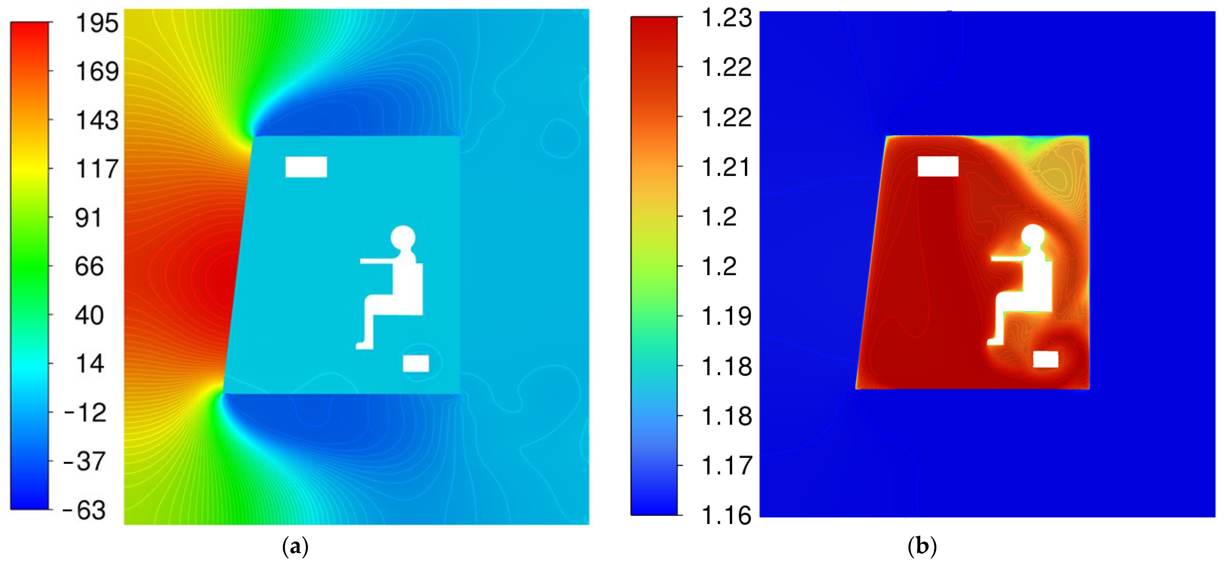
(a) Relative pressure, Pa; (b) air density, kg/m3.

Figure 5.
Velocity field, m/s: (a) in all domains; (b) in the cabin.

Figure 6.
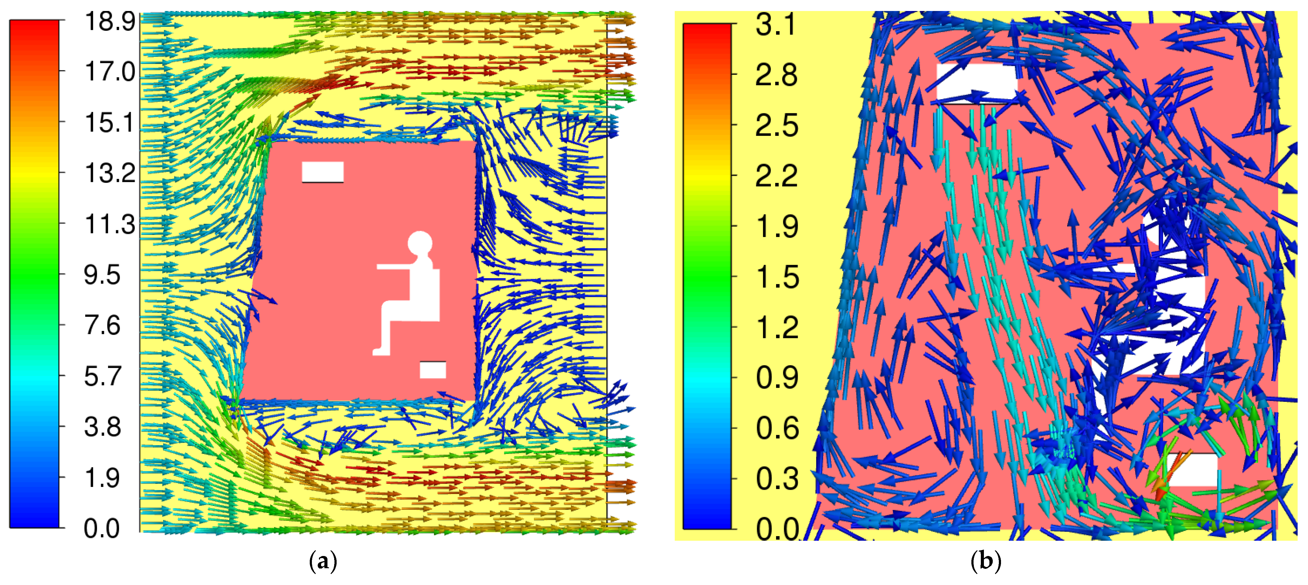
Vector velocity field, m/s: (a) in all domains; (b) in the cabin (directions and quantitative values of the parameters are shown by arrows in accordance with the color palette).
Figure 6.
Vector velocity field, m/s: (a) in all domains; (b) in the cabin (directions and quantitative values of the parameters are shown by arrows in accordance with the color palette).

Figure 7.
Temperature, °C: (a) in the cabin; (b) in all domains.

Figure 8.
Heat transfer coefficients on the left wall.

Figure 9.
Heat flux q on the left wall.
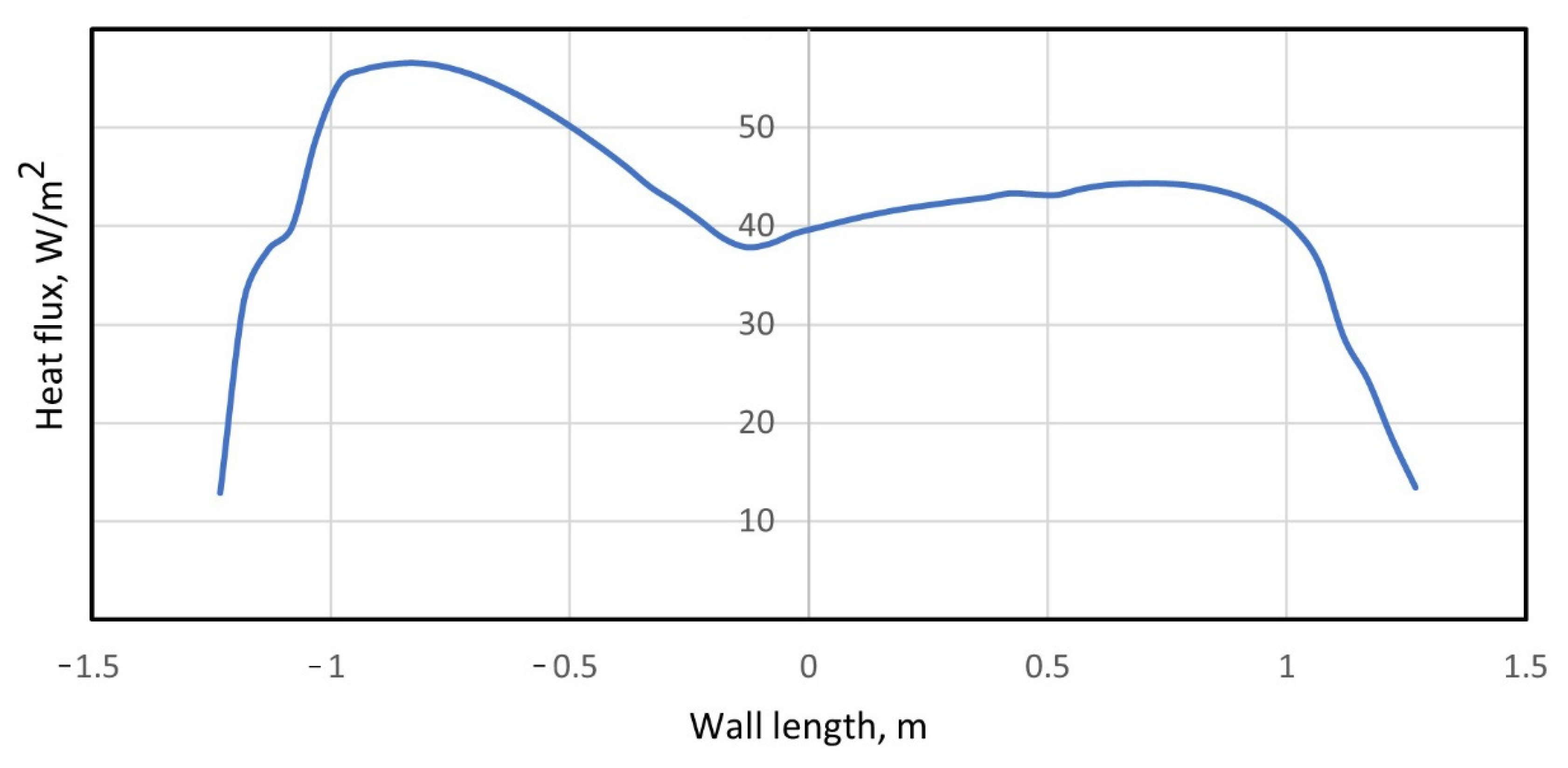
Figure 10.
Heat transfer coefficients on the top wall.

Figure 11.
Heat flux q on the top wall.
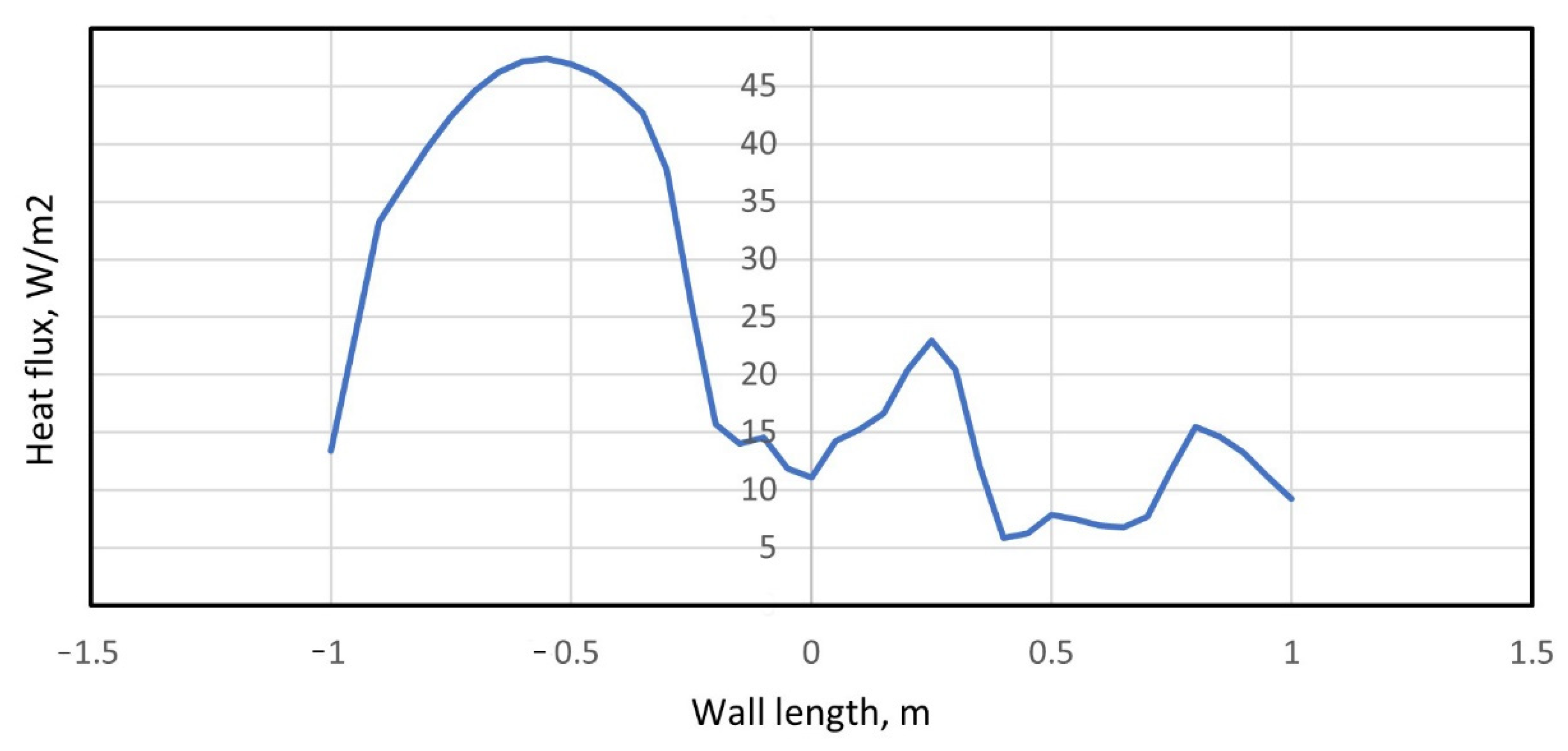
Figure 12.
Heat transfer coefficients on the right wall.

Figure 13.
Heat flux q on the right wall.

Figure 14.
Values of turbulent kinetic energy .

Figure 15.
Velocity near the wall: (a) region; (b) velocity.
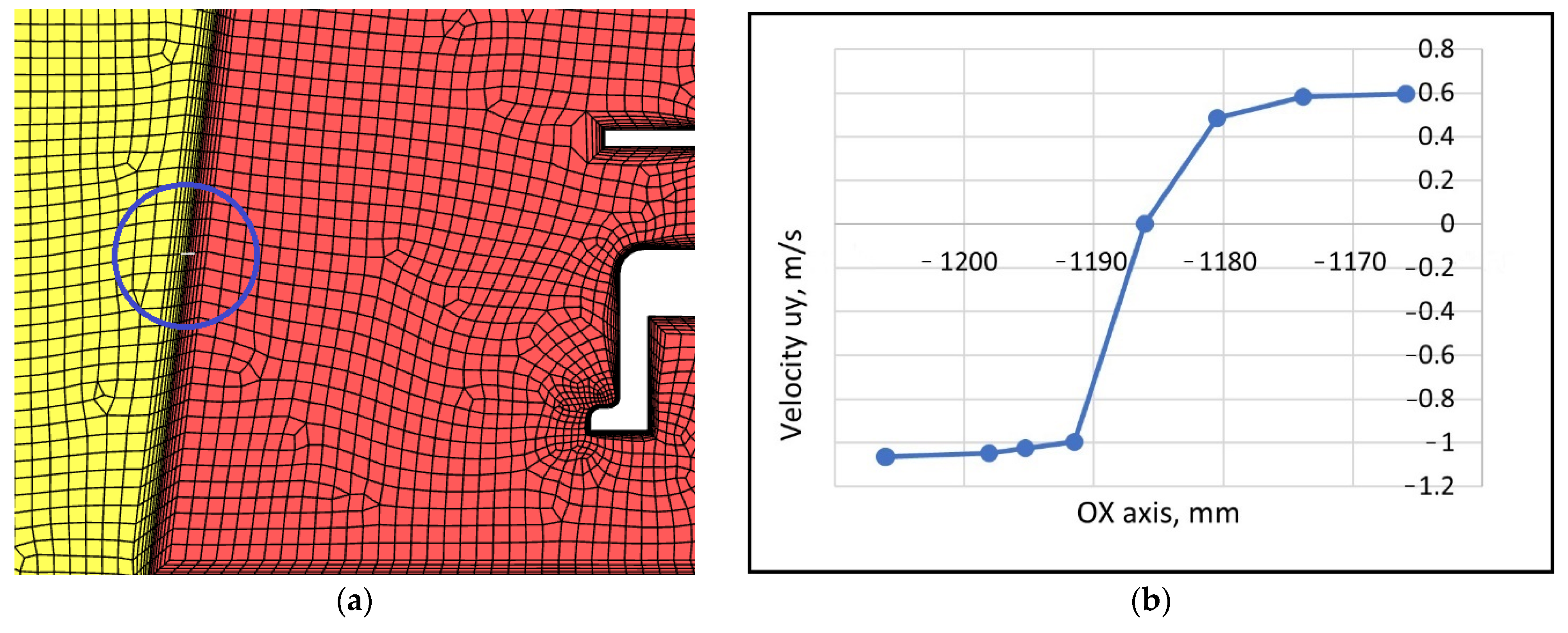
Figure 16.
Velocities along the left wall.

Figure 17.
Velocities along the top wall.

Figure 18.
Velocities along the right wall.
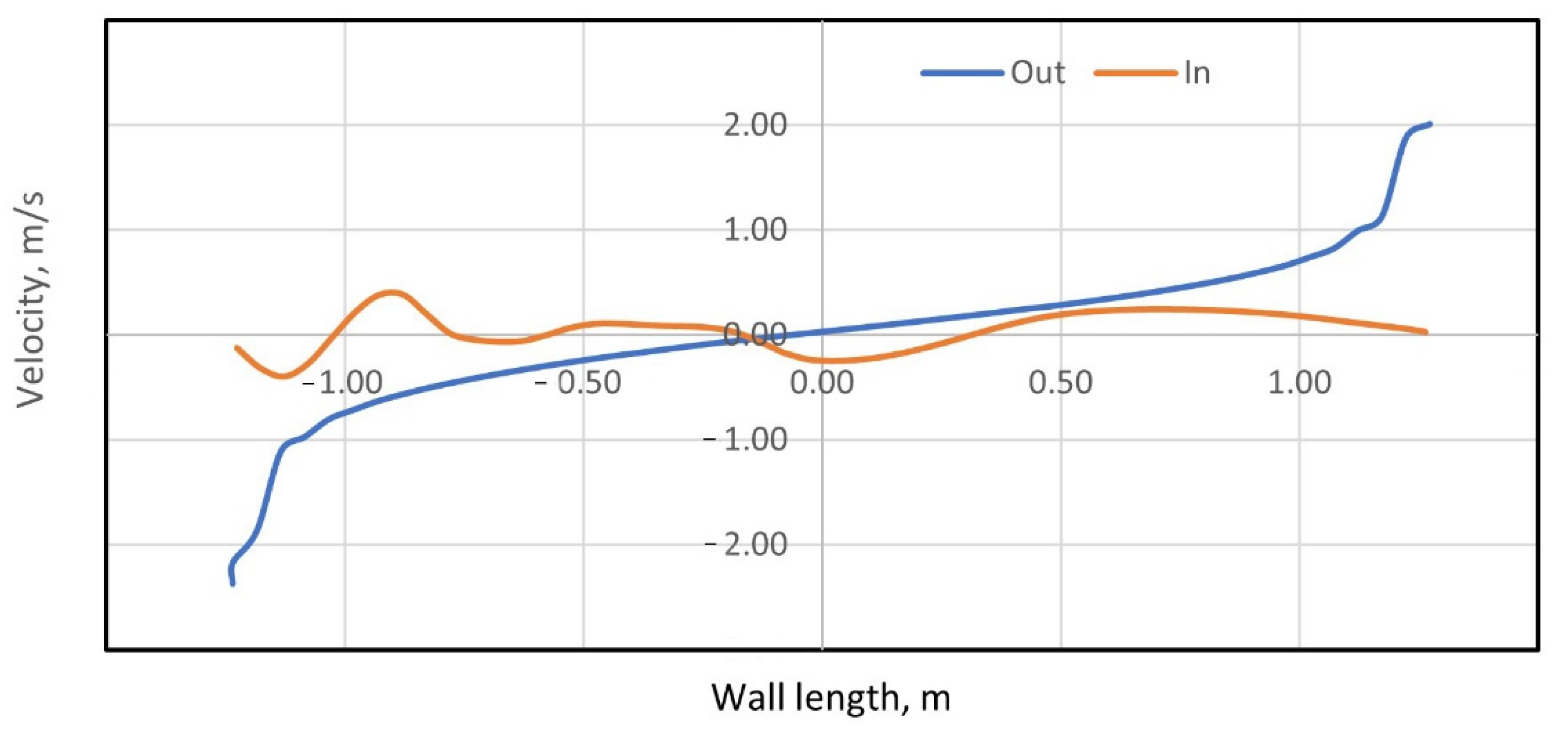
Figure 19.
Heat transfer coefficients for the left wall .

Figure 20.
Heat transfer coefficients for the left wall .
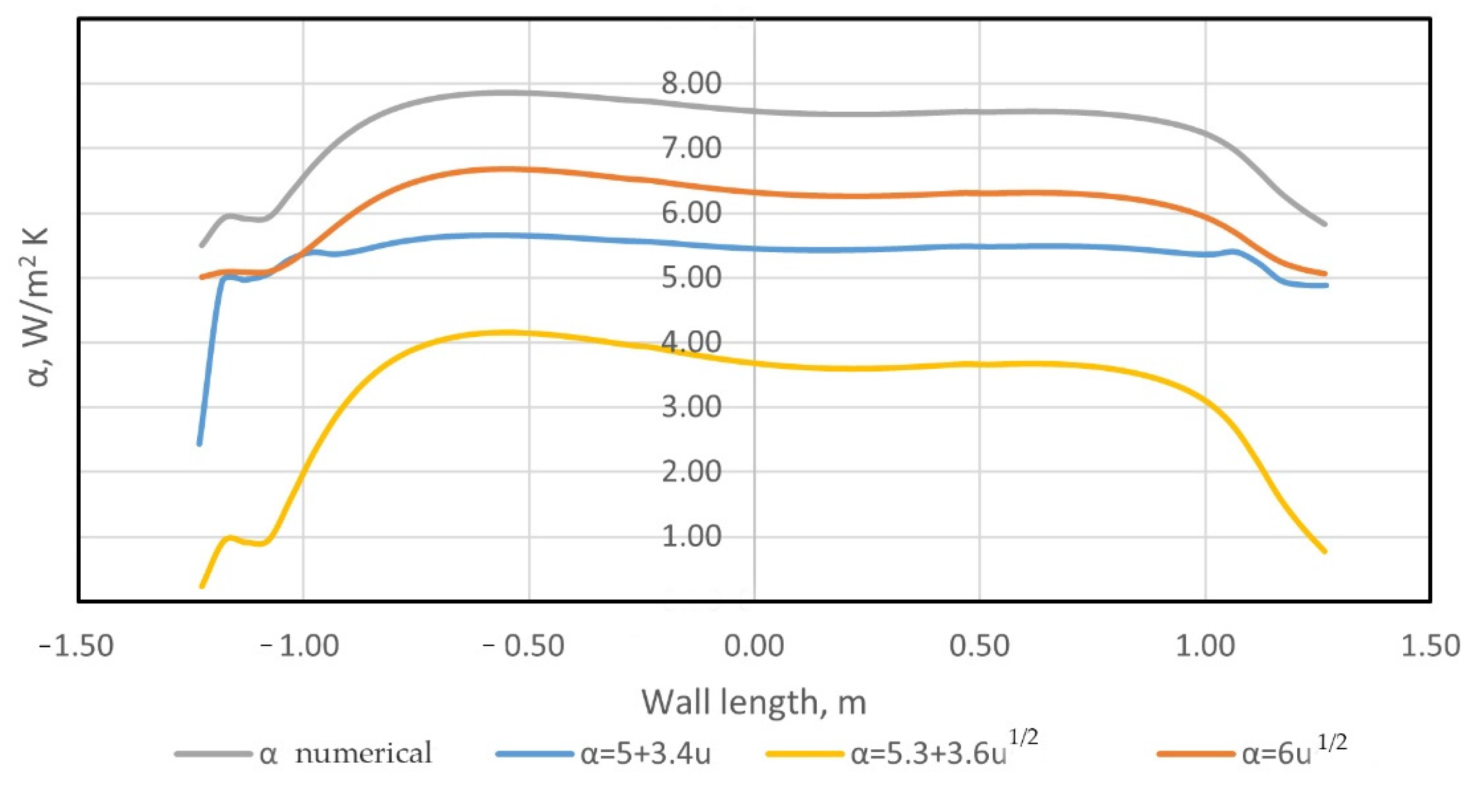
Figure 21.
Heat transfer coefficients for the top wall .

Figure 22.
Heat transfer coefficients for the top wall .

Figure 23.
Heat transfer coefficients for the right wall .
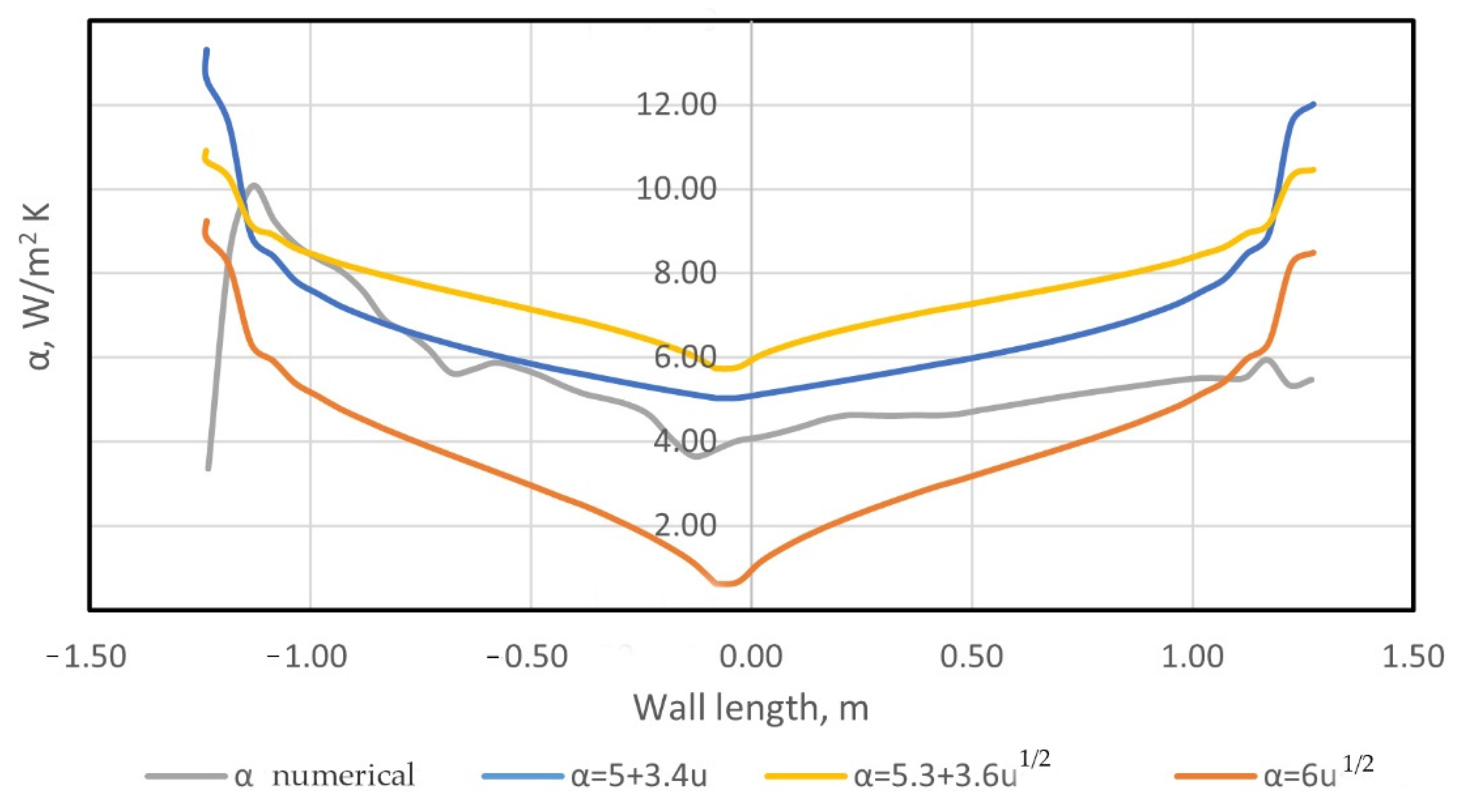
Figure 24.
Heat transfer coefficients for the right wall .

Table 1.
Wall parameters.
| Wall Material | Coefficient of Thermal Conductivity, | Thickness, m |
|---|---|---|
| Metal | 58 | 0.002 |
| Bituminous mastic layer | 0.27 | 0.0042 |
| Cast polyurethane | 0.32 | 0.025 |
Table 2.
Boundary conditions and environment parameters.
| No. | Title | Value |
|---|---|---|
| 1 | Free stream speed, m/s | 5 |
| 2 | Incoming flow temperature, °C | 30 |
| 3 | Air flow rate in cabins, m/s | 1 |
| 4 | Cabin air flow temperature, °C | 14 |
| 5 | Thermal conductivity of air, W/(m2∙K) | 0.0242 |
| 6 | Heat capacity of air, J/(kg∙K) | 1006.43 |
| 7 | Average temperature on the human surface, °C | 25 |
| 8 | Molar mass of air, kg/mol | 28.966 |
Table 3.
Values of the average heat transfer coefficients obtained by the numerical method and by applied formulas obtained experimentally.
Table 3.
Values of the average heat transfer coefficients obtained by the numerical method and by applied formulas obtained experimentally.
| Wall | Coefficient Type | ||||
|---|---|---|---|---|---|
| Left wall | 5.3 | 5.7 | 6.9 | 2.7 | |
| 18.9 | 22.0 | 13.3 | 13.4 | ||
| Top wall | 2.3 | 5.7 | 6.9 | 2.7 | |
| 21.0 | 22.0 | 13.3 | 13.4 | ||
| Right wall | 4.3 | 5.7 | 6.9 | 2.7 | |
| 5.6 | 22.0 | 13.3 | 13.4 |
Table 4.
Errors in the values of the average heat transfer coefficients obtained by the numerical method and by applied formulas obtained experimentally.
Table 4.
Errors in the values of the average heat transfer coefficients obtained by the numerical method and by applied formulas obtained experimentally.
| Wall | Coefficient Type | ||||
|---|---|---|---|---|---|
| Left wall | 5.3 | 7 | 23 | 49 | |
| 18.9 | 14 | 29 | 29 | ||
| Top wall | 2.3 | 60 | 67 | 15 | |
| 21.0 | 5 | 36 | 36 | ||
| Right wall | 4.3 | 25 | 38 | 37 | |
| 5.6 | 75 | 58 | 58 |
Publisher’s Note: MDPI stays neutral with regard to jurisdictional claims in published maps and institutional affiliations. |
© 2022 by the authors. Licensee MDPI, Basel, Switzerland. This article is an open access article distributed under the terms and conditions of the Creative Commons Attribution (CC BY) license (https://creativecommons.org/licenses/by/4.0/).
Share and Cite
MDPI and ACS Style
Beskopylny, A.N.; Panfilov, I.; Meskhi, B. Modeling of Flow Heat Transfer Processes and Aerodynamics in the Cabins of Vehicles. Fluids 2022, 7, 226. https://doi.org/10.3390/fluids7070226
AMA Style
Beskopylny AN, Panfilov I, Meskhi B. Modeling of Flow Heat Transfer Processes and Aerodynamics in the Cabins of Vehicles. Fluids. 2022; 7(7):226. https://doi.org/10.3390/fluids7070226
Chicago/Turabian StyleBeskopylny, Alexey N., Ivan Panfilov, and Besarion Meskhi. 2022. "Modeling of Flow Heat Transfer Processes and Aerodynamics in the Cabins of Vehicles" Fluids 7, no. 7: 226. https://doi.org/10.3390/fluids7070226