
Influence of Sill on the Hydraulic Regime in Sluice Gates: An Experimental and Numerical Analysis
by
 , , , and
Rasoul Daneshfaraz
1,* ,
,
Reza Norouzi
2 ,
,
Hamidreza Abbaszadeh
1 ,
,
Alban Kuriqi
3,4 and
and
Silvia Di Francesco
5 1
Department of Civil Engineering, Faculty of Engineering, University of Maragheh, Maragheh 5518183111, Iran
2
Department of Water Engineering, Faculty of Agriculture, University of Tabriz, Tabriz 5166616471, Iran
3
CERIS, Instituto Superior Técnico, Universidade de Lisboa, 1049-001 Lisboa, Portugal
4
Civil Engineering Department, University for Business and Technology, 10000 Pristina, Kosovo
5
Department of Engineering, Engineering Faculty, Niccolò Cusano University, 00166 Rome, Italy
*
Author to whom correspondence should be addressed.
Fluids 2022, 7(7), 244; https://doi.org/10.3390/fluids7070244
Submission received: 4 June 2022
/
Revised: 11 July 2022
/
Accepted: 15 July 2022
/
Published: 16 July 2022
Abstract
:This study investigates experimentally and numerically the effects of sills with different geometric specifications at various positions on the hydraulic characteristics of flow through sluice gates. The simulation results showed that the RNG turbulence model’s statistical indicators yield high accuracy compared to the k-ε, k-ω, and LES turbulence models. The discharge coefficient (Cd) has an inverse relationship with gate opening. Regarding sill state, the discharge coefficient is higher than no-sill state. In the case of non-suppressed sills, the Cd decreases compared to the smaller openings as the opening of the gate changes. The results showed that the Cd with a sill in the tangent position upstream of the gate is higher than the downstream tangent and below situations. Increasing the sill length leads to an increase in flow shear stress and consequently a decrease in Cd. The Cd of gates with different sill thicknesses is always higher than the no-sill state, but due to the constant ratio of the fluid depth above the sill to the gate opening, the Cd increases to a certain extent and then decreases with increasing sill thickness.
1. Introduction
Gates are hydraulic structures used to operate flow discharges from channels, weirs, and spillways, among others. The most common are sluice gates that move vertically up and down to adjust the opening regarding the flow that needs to be released. Determining the flow rate and estimating the discharge coefficient is one of the most important issues in hydraulic engineering. This information helps engineers to design the structure cost-effectively. Controlling the upstream fluid depth is based on the amount of gate opening. It is important for estimating the discharge coefficient. In recent decades, the optimization of water resources has become a more prevalent issue due to the scarcity of water resources. To prevent water wastage, the control and distribution of water in irrigation networks should be optimized. Double or triple gates are used when the gate height exceeds a certain design criterion (Negm et al. [1]); however, using these gates is very expensive. One of the basic solutions for dealing with this issue is to use a gate–sill combination. The sill affects the flow pattern by increasing the gates’ hydraulic performance and water distribution efficiency in irrigation networks.
Studies by Henry [2], Rajaratnam and Subramanya [3], Rajaratnam [4], and Swamee [5] on sluice gate discharge coefficients have provided relationships for estimating discharge coefficients. Alhamid et al. [6] showed that the discharge coefficients increase with a sill state compared to the no-sill state. Shivapur and Prakash [7] investigated the placement of sluice gates at different angles relative to the vertical axis. Their results showed that the discharge coefficient increases with increasing the angle. Mohammed and Moayed [8] investigated the gate edge’s effect and its orientation in the flow. The results showed that the discharge coefficient for a gate with an angle of 45° to the flow direction with a horizontal and sharp edge is 17.8% and 17% higher than the vertical gate, respectively. Daneshfaraz et al. [9] numerically investigated the effect of sluice gate edge shapes on flow characteristics. Their results indicated that the flow contraction coefficient for sharp edges and round-edge gates decreases when the ratio of gate opening to upstream specific energy is less than 0.4 and increases for ratios greater than 0.4. Reda [10] modeled the flow characteristics under vertical and inclined gates using artificial networks. They applied the ANN intelligence model as a suitable model for predicting the discharge coefficient for vertical and inclined sluice gates. Salmasi and Norouzi [11] investigated the effect of different geometric shapes of suppressed sills on sluice gate discharge coefficients. The results indicated that the circular sill is the most effective shape while the triangular sill is one of the best polygonal sills. Karami et al. [12] investigated the discharge coefficients of gates using FLOW-3D software. The results showed that the semicircular sill greatly affects the discharge coefficient and increases the discharge coefficient by 20%. Salmasi and Abraham [13] examined the discharge coefficient of sluice gates with polygonal and non-polygonal sills. They concluded that trapezoidal sills have the least effect on the discharge coefficient.
Pastor et al. [14] presented the procedure for assessing the safe operation of the sluice gate, on which places with permanent deformation and a broken part of the guide wheel flange were identified. Using numerical modeling, they identified critical stress values at the locations of reinforcing elements, which were modified. The stress values were reduced by about 15%. Ghorbani et al. [15] analyzed the discharge coefficient of sluice gates with the sill state using the H2O method and intelligent models such as DL, RF, GBM, and GL. Based on their results, the H2O machine learning method yields good performance for estimating the discharge coefficient. Daneshfaraz et al. [16] examined the position of the gates, including vertical or inclined/oblique gates. They reported better performance for upward inclined positions than other gate positions in discharge coefficient increases. Kubrak et al. [17] analyze the possibilities of using an irrigation sluice gate in submerged conditions to measure water flow rate. Based on their results, relationships for discharge coefficients of the analyzed sluice gate were developed. Salmasi et al. [18] used experimental data and intelligence models to investigate the gate discharge coefficient. Lauria et al. [19] investigated broad crested weirs’ sluice gate discharge coefficient. Based on their results, it is possible to identify the minimal opening of the gate such that viscous effects can be neglected. Salmasi and Abraham [20] conducted laboratory experiments to determine the discharge coefficient for inclined slide gates. Their results showed that the inclination of the slide gates has a progressive effect on discharge coefficient and increases capacity through the gate. Silva and Rijo [21] used different discharge estimation methods. Their results show that the discharge assessment under the sluice gates for free and submerged flow conditions using energy models had better accuracy.
This study provides a general formula for calculating the discharge coefficient through gates with various sill states. The effect of sill geometry, sill opening, and relative position of the sill are investigated. The need to investigate sluice gates without and with suppressed and non-suppressed sill states will be investigated experimentally and numerically using the VOF method. The effect on hydraulic parameters capacity, hydrodynamic force, shear stress, and discharge coefficient are provided.
2. Materials and Methods
2.1. Experimental Equipment
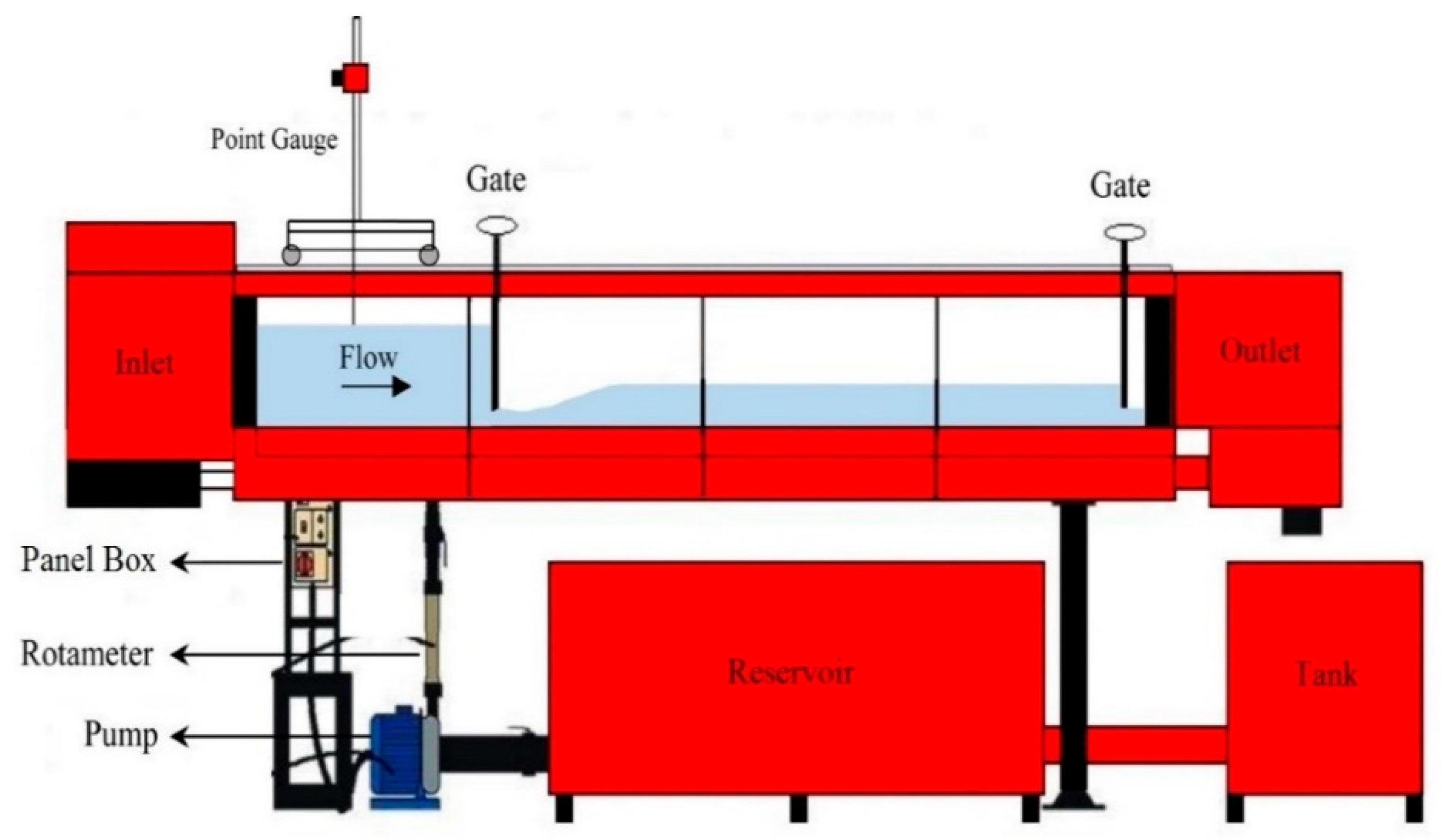
An experimental flume with a rectangular cross-section 5 m long, 0.3 m wide, and 0.5 m deep was fabricated with transparent Plexiglas walls and floors, facilitating the flow observation. The slope of the channel floor was adjustable and set to zero for the experiments. Two pumps, each with a nominal capacity of 450 L/min, were used to supply the input flow to the flume. Rotameters installed on the flume were used to measure flow rates with ±2% accuracy. Several parallel calming plates were used at the flume’s beginning to reduce the flow turbulence. Here, a point depth gauge with a reading accuracy of ±1 mm was used to measure the water depth in the flume (Figure 1). To increase the measurement accuracy, depths were measured at 4 locations of the cross-section, and their average was considered to be the final depth. The experiments were performed both with and without sill gates. In this study, 412 experiments were performed over a flow range of 150 to 850 L/min. This study performed experiments using polyethylene sills under the gate and upward and downward tangent gate positions (Figure 2 and Figure 3b). A series of photographs of the experimental facility is provided in Figure 2.
2.2. Relation Related to Flow Passing through the Sluice Gate
The flow rate through the sluice gate with a suppressed sill is calculated according to Equation (1) (Alhamid [6], Salmasi and Abraham [13]):
In Equation (1), Q is the discharge (L3T−1), Cd is the discharge coefficient (-), W is the channel width (L), G is the gate opening (L), g is the gravitational acceleration (LT−2), H0 is the upstream water depth (L), and Z is the sill height (L). For the no-sill case, Z is equal to zero; therefore, the sluice gate discharge equation with the no-sill case is written (Rajaratnam and Subramanya [3], Swamee [5]):
In Equations (1) and (2), WG is the area of opening (L2). According to Equation (2), the flow rate through the gate with suppressed sill is calculated based on the fluid depth over the sill (H0 − Z). Equation (3) calculates the flow rate through the gate with the non-suppressed sill.
In Equation (3), the symbols A1 = b1G1, A3 = b3G1, and A2 = BG2 are the flow area in, beside, and over the sill (L2), respectively. Figure 3 shows a sluice gate without and with a sill state relative to the gate.
In Figure 3, B is the sill width (L), ε is the sill thickness (L), y0 is the water depth above the sill (L), and Atotal is the total flow area under the gate (L2), which is equal to Atotal = A1 + A2 + A3.
2.3. Flow Governing Equations
The continuity and Navier–Stokes equations are discretized by FLOW-3D software to perform a three-dimensional simulation of fluid motion. The continuity equation in a fluid flow is in the form of Equation (4) (Flow Science Inc., Santa Fe, NM, USA. [22]).
where ui is the velocity component in the direction i. For 3D flow analysis, the software solves Navier–Stokes equations using the finite volume method. Navier–Stokes equations are momentum equations governing the flow of viscous Newtonian fluids. This Equation is generally expressed as Equation (5) (Daneshfaraz et al. [16]).
where Bi is the volumetric force in direction i, µ is the fluid’s dynamic viscosity, xi, xj, and xk are the flow coordinates in the spatial direction i, j, and k, respectively. δij represents the Kronecker delta; if i = j, its value is 1; otherwise, it has a value equal to zero.
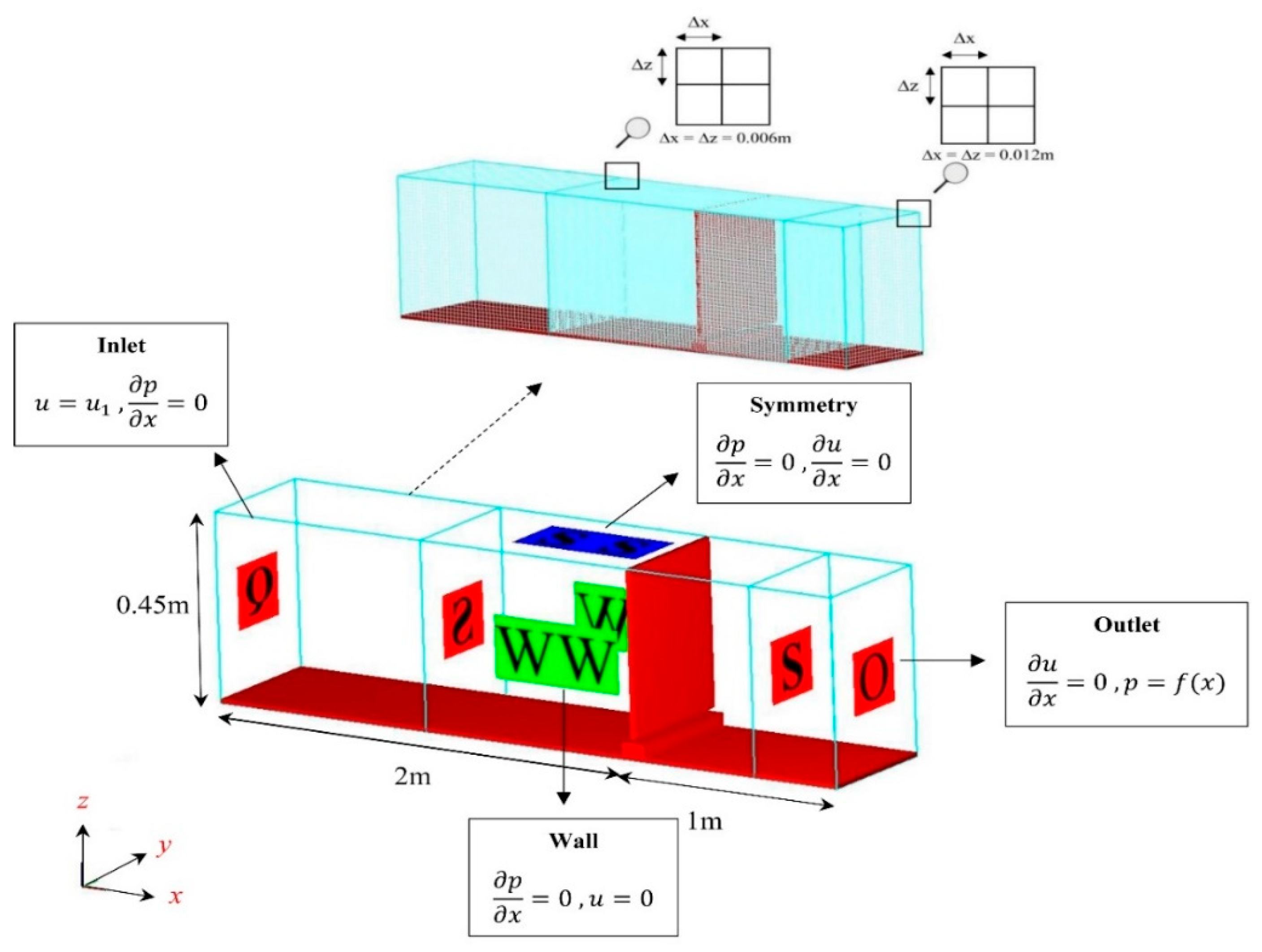
2.4. Defining the Solution Network, Boundary Conditions, and Selecting the Turbulence Model
In this study, data validation was performed by comparing the experimental results to the simulations. Next, the simulations were continued for other models of the present study. Table 1 shows the hydraulic and geometric characteristics of the studied models. The 3-D geometry of the model and meshing geometry is shown in Figure 4.
The simulations have been conducted with nested mesh blocks with different dimensions. The volume flow rate boundary condition was used for the inlet condition, and a standard output boundary condition was used at the downstream end of the channel. The wall boundary condition is selected at the channel’s walls and floor. For the upper boundary, symmetric boundary conditions are applied. At the interface between meshed regions, flow continuity is enforced. The symmetry boundary condition is defined for the second mesh block’s inlet, output, and upper boundary. In addition, the wall boundary condition is selected for the walls and the floor of the channel.
To achieve the optimal mesh, simulations were performed in different element dimensions. A comparison of numerical solution results with experimental results is given in Table 2. To select the turbulence model, simulations were performed with four turbulence models of RNG, k-ε, k-ω, and LES (Table 3). The RNG turbulence model was the most appropriate for using similar approaches [16,23,24,25,26,27]. A comparison of the quantitative simulation results of the turbulence models mentioned in Table 3 shows that the RNG turbulence model produces less error than other turbulence models and is closer to the experimental results. The statistical indicators of percentage relative error (RE%), root mean square error (RMSE), and Kling Gupta efficiency (KGE) were used to evaluate the performance of the model in simulation, and the results were compared with experiments:
In the above relations, Obs and Cal indicate the observational and numerical solution results (computational), respectively; n is the total number of data. Equations (6) and (7), which are close to zero, indicate the high accuracy of the numerical solutions. In Equation (8), R represents the correlation coefficient, and β is the ratio of the computational data’s mean to the observational data’s mean. The γ represents the ratio of the computational values’ standard deviation to the observational values’ standard deviation. The KGE statistical index can be categorized into very good, good, satisfactory, acceptable, and unsatisfactory to indicate the relationships’ accuracy.
3. Results and Discussion
3.1. Validation Results
According to the initial and boundary conditions, the numerical simulation initiates at non-steady conditions. Then, it converges until the flow reaches a steady state (Figure 5). According to the continuity equation, at a given volume over a given period, the change in fluid mass is equal to the difference between the mass of the inlet fluid and the mass of the outlet fluid. According to the discharge–time hydrograph, it is observed that the flow fluctuates considerably in the initial phase. However, with the continuation of the process, it becomes stable.
Table 2 shows the validity results between experimental and numerical solution values for different mesh sizes and statistical indicators related to each size. According to Table 2 and the statistical indicators analysis, it was observed that Test No. 5 has favorable conditions in terms of the Mean RE%, RMSE, and KGE, and is superior to other tests. Considering that the statistical indicators for 4 and 5 are very close to each other, Test No. 4 is considered the optimal mesh with mesh dimensions of 0.012 and 0.006 m to continue the simulation process of the studied models. In selecting the optimal mesh size (Table 2), a turbulence model is first assumed (based on experience and previous studies, the RNG turbulence model was assumed). After obtaining the optimal mesh size, various turbulence models were checked (Table 3).
After finding the optimal mesh (Test No. 4) and based on it, different turbulence models were simulated (Table 3). The best and optimal turbulence model was selected by comparing the obtained statistical indicator. A comparison of the quantitative simulation results of the turbulence models mentioned in Table 3 shows that the RNG turbulence model has less error than other turbulence models and is closer to the experimental results.
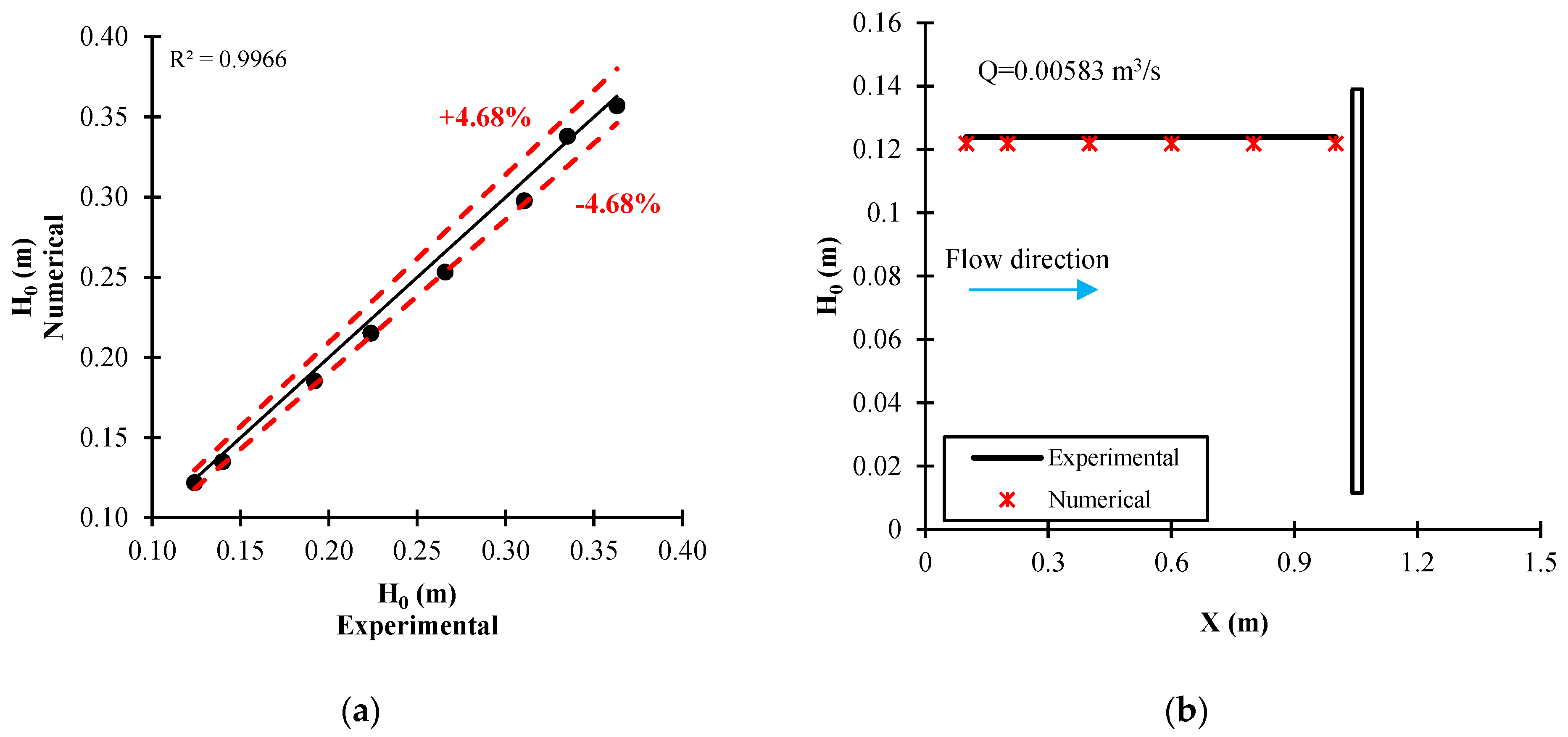
Table 4 shows the dissociation results of the percentage relative error for each of the simulations performed with the optimal mesh compared to the corresponding experimental results. One of the most significant factors affecting the sluice gate discharge coefficient is the upstream fluid depth and gate opening (Swamee [5]). By writing the Bernoulli Equation for sections behind and after the gate, and ignoring no loss between them, Equations (1)–(3) are obtained. By validating the experimental results obtained from Equation (3) and the numerical solution, a desirable match was seen between the results of the upstream depth and the discharge coefficient. In addition, among other factors affecting the discharge coefficient with sill are the shear stress, upstream flow velocity, and the geometric characteristics of the sill, which directly affect the upstream water depth and, consequently, the discharge coefficient.
Figure 6 shows the numerical solution calibration compared to the laboratory results for the upstream water depth and the longitudinal profile of the flow upstream of the gate. As shown in Figure 6, there is a good agreement between the results so that the R2 and the maximum percentage relative error are 0.996 and ±4.68%, respectively.
3.2. Discharge Coefficient of the Gate with No-Sill Case
The experimental results were evaluated using the dimensionless parameter (Cd) and the ratio of the upstream depth to gate opening (H0/G). According to Figure 7a, the values of the Cd are inversely related to the gate opening. Figure 7b shows the stage–discharge diagram for the various openings of the sluice gate in the no-sill case. The gate opening is inversely related to the upstream water depth at a certain flow rate. As it increases, the fluid depth decreases. For an opening of 1 cm, the average Cd value is higher than the openings of 2, 4, and 5 cm by 7.75%, 16.51%, and 18.35%. Similarly, the maximum values of Cd are 16.62%, 28.9%, and 23.51%, respectively.
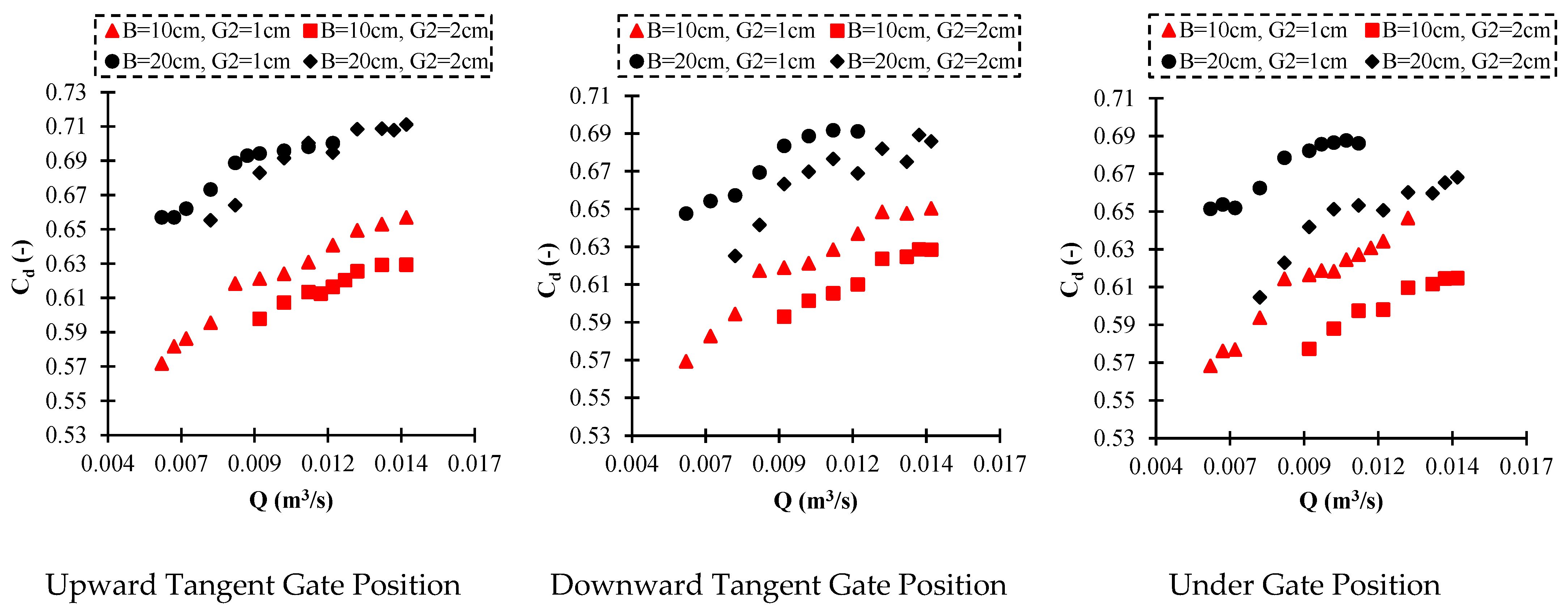
3.3. Discharge Coefficient of the Gate with Suppressed and Non-Suppressed Sill Case
Figure 8 investigates the effect of suppressed and non-suppressed sills on the Cd for a sluice gate in different positions. According to Figure 8, for a sill below and tangential to the gate, Cd increases with increasing sill width. A sill with the smallest width has a minimum value of the coefficient. By increasing the upstream fluid depth ratio to the sill width, Cd has an increasing trend. By comparing the Cd in different positions, the discharge coefficient in the upward tangent position of the sill is higher than the position below the sluice gate. The reason for this is the placement of the sill. In the tangent position, the entire thickness of the sill is located behind the gate, so that a larger volume of water passes through the gate. In the below position, half of the sill is located after the gate so that it acts as a barrier and increases the friction coefficient of the flow. This consequently increases the fluid depth upstream of the gate more than in the tangent position. For the downward tangent gate position compared to the sill below position, Cd is higher and lower than the upward tangent gate position. As in the upward tangent gate position, the upstream fluid depth is less than for the below and downward tangent gate positions. The greatest depth is related to the sill below the gate. Therefore, the non-suppressed sill of the tangential model can be used due to its optimal performance in terms of increasing the efficiency of the flow rate and preventing the accumulation of sediments behind the gate.
In order to present the results, the rate of change of Cd with different discharges and positions is presented for some of the sills. In addition, the effect of the gate opening with sill is investigated in Figure 9. Comparison of the Cd for different openings with a sill in different positions indicates a decrease in Cd compared to the gate with a lesser opening. In all sill placement models, the maximum value is related to the upward tangent gate position.
In Figure 10a,b, a comparison was drawn between the sluice gate discharge coefficient without a sill and with suppressed sills at the same opening. In Figure 10a, the opening is 1 cm. Figure 10b shows the changes in the discharge coefficient for an opening of 2 cm with and without a sill. According to Figure 10, it can be seen that the presence of a sill below and tangential to the sluice gate compared to the no-sill state increases the flow rate and improves system performance in terms of permeability. The highest value is the sill upward gate position (i.e., behind the gate). Since the position of the sill changes, the streamlines have a significant effect on the Cd. Streamlines behind the gate for the tangential position continue a smooth tangential trajectory and experience a relatively smaller energy loss.
On the other hand, in the tangential position after the gate and the below position, flow passes over the sill as a jet and eddies form, leading to greater energy loss. Increasing the contact length of the flow with the sill increases the friction and resistance of the output flow through the gate. It increases upstream depth (Figure 11). For a constant discharge, the upstream fluid depth in all sill positions is less than without a sill. As the upstream depth increases, the flow through the gate has a higher pressure, which causes additional losses. Heterogeneous rotating currents downstream of the gate lead to a decrease in the discharge coefficient. The presence of a sill also causes the pressure on the gate to be less than γH0. Therefore, reducing the pressure and suction of the flow leads to an increase in the discharge coefficient.
3.4. Hydraulic Parameters of the Gate with Various Geometry of the Sill
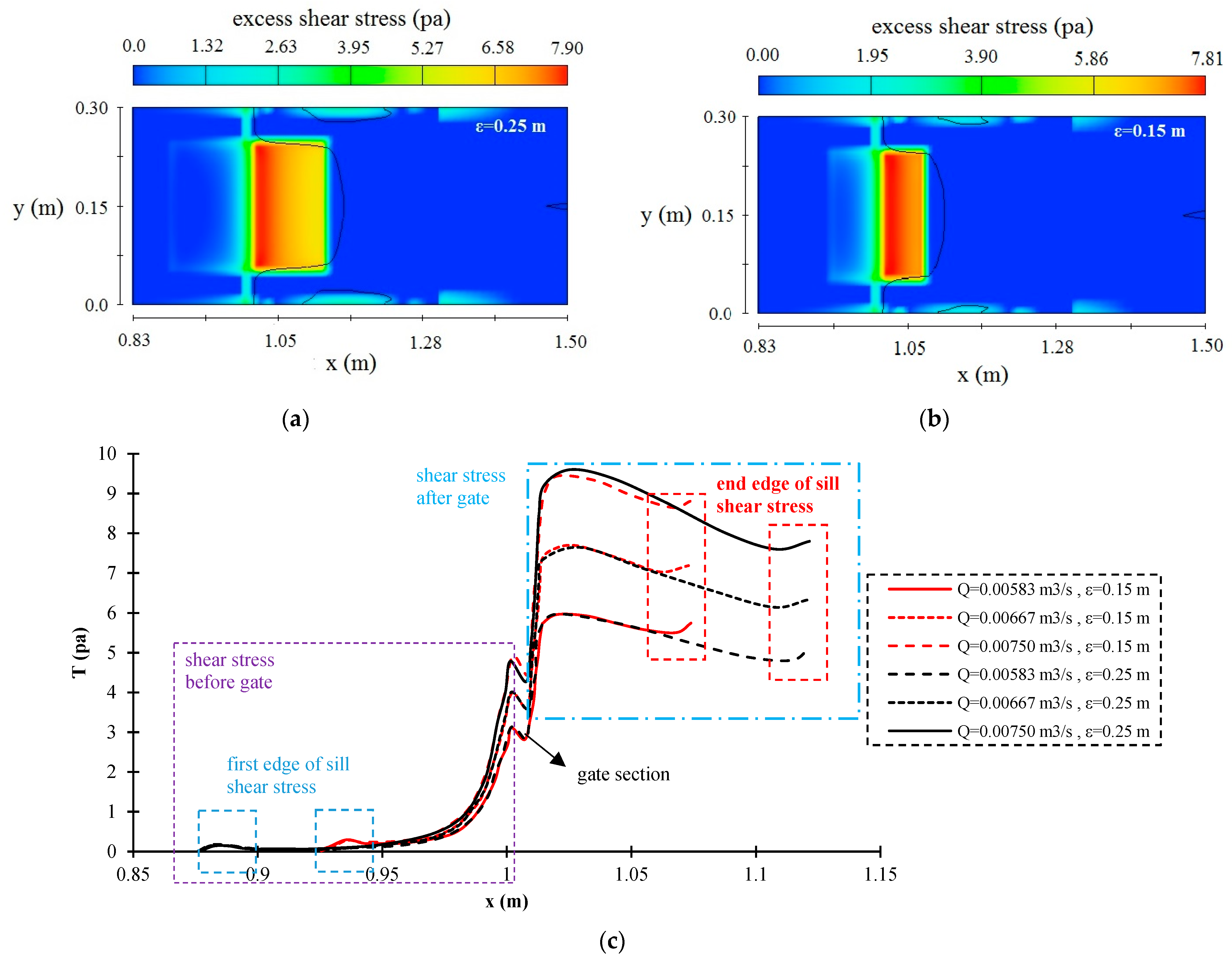
The channel cross-section near the gate’s back is presented according to Figure 12 for the non-suppressed sill state with different thicknesses of 0.05, 0.15, and 0.25 m in various discharges. At the same discharge, as the sill thickness increases, the average flow velocity decreases, which leads to an increase in the upstream depth. In other words, according to Figure 13, which shows the position of shear stress around and along the sill at the level near its surface in the center of the channel, increasing the sill thickness increases the shear stress. In Figure 13c, the shear stress behind the gate increases as it approaches the gate. Moreover, at the beginning of the sill, the shear stress increased slightly due to the proximity to the sill wall; this sudden increase is also seen at the end of the sill. Downstream from the gate, the shear stress increases and decreases along the sill. In addition, according to Figure 13a,b, it is observed that increasing the sill thickness has a positive effect on increasing the shear stress on the surface and sides of the sill, so that the amount of shear stress in the boundary layer on both sides of the sill also exists and decreases with distance from it. This issue has also clearly shown its effect on the discharge coefficient. The increase in thickness has led to a decrease in the discharge coefficient (Figure 14a). In the suppressed sill, there is very little shear stress. The shear stress is only due to the sill thickness and channel walls (Figure 14b). Figure 14b compares the no-sill case with the suppressed sill. The presence of a sill increases the discharge coefficient. Consequently, the fluid depth behind the gate decreases compared to the no-sill case, reducing the compressive force on the gate.
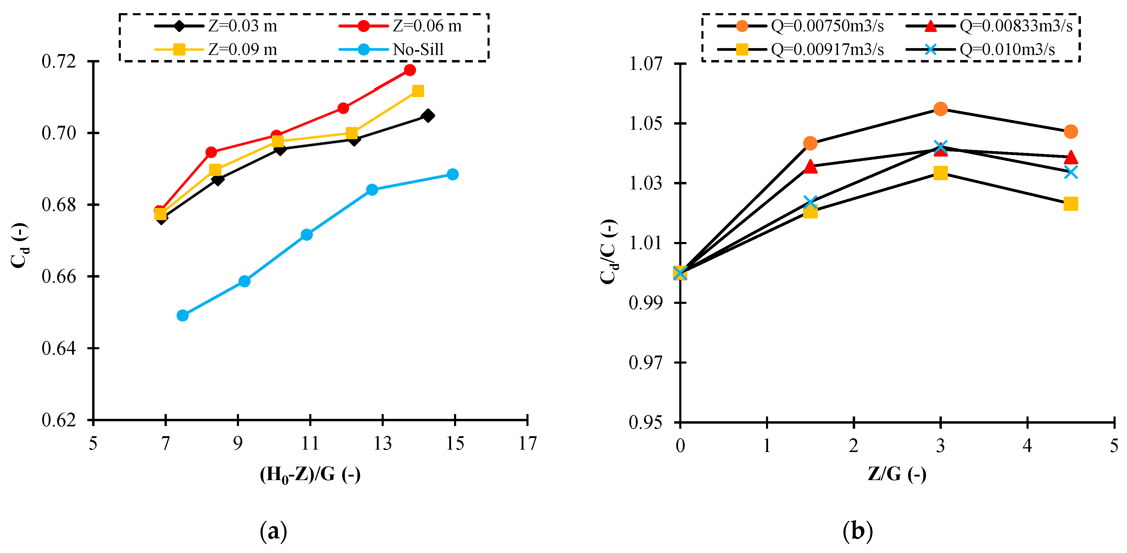
Figure 15a shows the effect of sill height on the discharge coefficient. Sill heights of 0.03, 0.06, and 0.09 m were considered. As can be seen, the discharge coefficient is higher in all silled cases. In addition, the sluice gate discharge coefficient increases with increasing the sill height to 0.06 m for all discharges but decreases at the sill with a thickness of 0.09 m compared to the sill with a height of 0.06 m. In this regard, Alhamid [6] also concluded that increasing the sill diameter increases and decreases the discharge coefficient. Figure 15b shows the effect of the ratio of sill height to gate opening on increasing the gate discharge coefficient. It should be noted that the variables Cd and C are related to the gate discharge coefficient with and without a sill, respectively. Increasing the ratio of Z/G initially increases the discharge coefficient, so that, at Z/W = 3, the sill has a maximum effect on the discharge coefficient. In addition, for ratios greater than Z/G > 3, the increase in discharge coefficient is less.
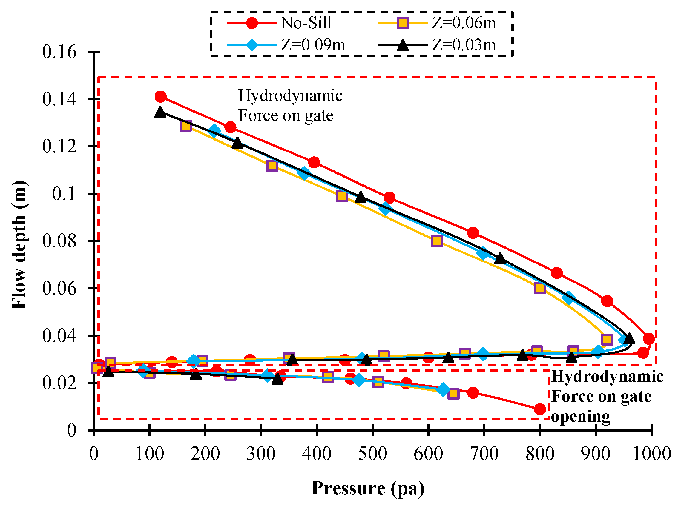
According to Figure 16, at a fixed discharge, as the sill height increases, the flow depth increases relative to the channel floor but decreases relative to the sill level. Concerning the flow rate calculation through the gate, the water depth over the sill is used, so the discharge coefficient increases compared to the no-sill state. The application of the sill also changes the pressure field upstream and downstream of the gate. As the height of the sill increases, the water depth relative to the bottom of the channel increases, and consequently, the pressure on the bottom of the channel increases. However, applying the sill causes a decrease in pressure and even negative pressure near the gate opening. This reduction in pressure in the areas close to the opening causes suction. It reduces the depth of water upstream of the gate. Figure 16 shows the pressure distribution on the gate for a flow rate of 0.00667 m3/s. As can be seen, with the construction of the sill, the pressure on the gate and the opening section is reduced. In addition, the pressure distribution is hydrostatic, but near the gate’s opening, the pressure distribution becomes hydrodynamic.
4. Conclusions
Experimental and numerical simulations using FLOW-3D were conducted to investigate the influence of a sill with various geometry in different positions, based on a preliminary assessment of the best and optimal (RNG) turbulence model. Our findings show that placing a sill before a sluice gate significantly affects the flow regime. Specifically, the following main conclusions can be drawn from this study:
- Out of the three studied sill positions, the under-gate sill case has a lower discharge coefficient than other sill positions.
- A comparison of discharge coefficients obtained from the application of sills showed that the highest value of discharge coefficients is related to the tangential model upstream of the gate. In the suppressed sill case, on average, the value of discharge coefficient for the upward tangential sill, downward tangential sill, and under gate sill positions are 0.779, 0.731, and 0.686, respectively.
- The flow depth upstream of the gate in the tangential upward position has the lowest value compared to other sill positions, leading to an increased discharge coefficient.
- The discharge coefficient is higher when the suppressed sill is broader and thicker until specified thicknesses and then begins to decrease. This conclusion is based on using various sill dimensions as well as the constant ratio of upstream fluid depth to the gate opening.
- By increasing the length of the suppressed and non-suppressed sill, the shear stress increases, and the value of the discharge coefficient decreases.
Moreover, the placement of the sill also changes the pressure field upstream and downstream of the gate. It was found that, as the height of the sill increases, the water depth relative to the bottom of the channel increases, and consequently the pressure on the bottom of the channel increases. However, applying the sill causes a decrease in pressure and even negative pressure near the gate opening. This reduction in pressure in the areas close to the opening causes suction. It reduces the depth of water upstream of the gate.
In natural conditions, the channel’s friction also significantly influences the flow regime’s different hydraulic parameters. Therefore, experimental channels with friction close to the natural conditions should be considered in future studies to have a clear picture of how the sill in front of the sluice gate would affect the hydraulic regime. Finally, solution-oriented findings from this study will help engineers design cost-effective hydraulic gates that operate under varied flow regimes.
Author Contributions
Conceptualization, R.D., R.N., H.A. and S.D.F.; methodology, R.D., R.N. and H.A.; formal analysis, R.D., R.N. and H.A.; investigation, R.D., R.N., H.A., A.K. and S.D.F.; data curation, H.A.; writing—original draft preparation, R.D., R.N., H.A., A.K. and S.D.F.; writing—review and editing, R.D., R.N., H.A., A.K. and S.D.F.; supervision, R.D.; project administration, H.A. All authors have read and agreed to the published version of the manuscript.
Funding
This research received no external funding.
Institutional Review Board Statement
Not applicable.
Informed Consent Statement
Not applicable.
Data Availability Statement
Data are contained within the article.
Conflicts of Interest
The authors declare no conflict of interest.
References
- Negm, A.M.; Alhamid, A.A.; El-Saiad, A.A. Submerged flow below sluice gate with sill. In Proceedings of the International Conference on Hydro-Science and Engineering Hydro-Science and Engineering ICHE98, Cottbus/Berlin, Germany, 31 August–3 September 1998; University of Mississippi: Oxford, MS, USA, 1998. Advances in Hydro-Science and Engineering. Volume 3. [Google Scholar]
- Henry, H.R. Discussion on “Diffusion of submerged jets” by Albertson, M.L. et al. Trans. Am. Soc. Civ. Eng. 1950, 115, 687. [Google Scholar]
- Rajaratnam, N.; Subramanya, K. Flow Equation for the Sluice Gate. J. Irrig. Drain. Div. 1967, 93, 167–186. [Google Scholar] [CrossRef]
- Rajaratnam, N. Free Flow Immediately Below Sluice Gates. J. Hydraul. Div. 1977, 103, 345–351. [Google Scholar] [CrossRef]
- Swamee, P.K. Sluice Gate Discharge Equations. J. Irrig. Drain. Eng. 1992, 118, 56–60. [Google Scholar] [CrossRef]
- Alhamid, A.A. Coefficient of Discharge for Free Flow Sluice Gates. J. King Saud Univ. Eng. Sci. 1999, 11, 33–47. [Google Scholar] [CrossRef]
- Shivapur, A.V.; Shesha Prakash, M.N. Inclined sluice gate for flow measurement. ISH J. Hydraul. Eng. 2005, 11, 46–56. [Google Scholar] [CrossRef]
- Mohammed, A.; Moayed, K. Gate Lip Hydraulics under Sluice gate. Mod. Instrum. 2013, 2, 16–19. [Google Scholar] [CrossRef] [Green Version]
- Daneshfaraz, R.; Ghahramanzadeh, A.; Ghaderi, A.; Joudi, A.R.; Abraham, J. Investigation of the Effect of Edge Shape on Characteristics of Flow Under Vertical Gates. J. Am. Water Work. Assoc. 2016, 108, E425–E432. [Google Scholar] [CrossRef]
- Reda, A.E.R. Modeling of flow characteristics beneath vertical and inclined sluice gates using artificial neural networks. Ain Shams Eng. J. 2016, 7, 917–924. [Google Scholar]
- Salmasi, F.; Norouzi Sarkarabad, R. Investigation of different geometric shapes of sills on discharge coefficient of vertical sluice gate. Amirkabir J. Civ. Eng. 2020, 52, 21–36. [Google Scholar] [CrossRef]
- Karami, S.; Heidari, M.M.; Adib Rad, M.H. Investigation of Free Flow under the Sluice Gate with the Sill Using Flow-3D Model. Iran. J. Sci. Technol. Trans. Civ. Eng. 2020, 44, 317–324. [Google Scholar] [CrossRef]
- Salmasi, F.; Abraham, J. Prediction of discharge coefficients for sluice gates equipped with different geometric sills under the gate using multiple non-linear regression (MNLR). J. Hydrol. 2020, 597, 125728. [Google Scholar] [CrossRef]
- Pástor, M.; Bocko, J.; Lengvarský, P.; Sivák, P.; Šarga, P. Experimental and Numerical Analysis of 60-Year-Old Sluice Gate Affected by Long-Term Operation. Materials 2020, 13, 5201. [Google Scholar] [CrossRef]
- Ghorbani, M.A.; Salmasi, F.; Saggi, M.K.; Bhatia, A.S.; Kahya, E.; Norouzi, R. Deep learning under H2O framework. A novel approach for quantitative analysis of discharge coefficient in sluice gates. J. Hydroinformatics 2020, 22, 1603–1619. [Google Scholar] [CrossRef]
- Daneshfaraz, R.; Abbaszadeh, H.; Gorbanvatan, P.; Abdi, M. Application of Sluice Gate in Different Positions and Its Effect on Hydraulic Parameters in Free-Flow Conditions. J. Hydraul. Struct. 2021, 7, 72–87. [Google Scholar] [CrossRef]
- Kubrak, E.; Kubrak, J.; Kiczko, A.; Kubrak, M. Flow Measurements Using a Sluice Gate; Analysis of Applicability. Water 2020, 12, 819. [Google Scholar] [CrossRef] [Green Version]
- Salmasi, F.; Nouri, M.; Sihag, P.; Abraham, J. Application of SVM, ANN, GRNN, RF, GP and RT Models for Predicting Discharge Coefficients of Oblique Sluice Gates Using Experimental Data. Water Supply 2021, 21, 232–248. [Google Scholar] [CrossRef]
- Lauria, A.; Calomino, F.; Alfonsi, G.; D’Ippolito, A. Discharge Coefficients for Sluice Gates Set in Weirs at Different Upstream Wall Inclinations. Water 2020, 12, 245. [Google Scholar] [CrossRef] [Green Version]
- Salmasi, F.; Abraham, J. Expert System for Determining Discharge Coefficients for Inclined Slide Gates Using Genetic Programming. J. Irrig. Drain. Eng. 2020, 146, 06020013. [Google Scholar] [CrossRef]
- Silva, C.O.; Rijo, M. Flow rate measurements under sluice gates. J. Irrig. Drain. Eng. 2017, 143, 06017001. [Google Scholar] [CrossRef] [Green Version]
- Flow Science Inc. FLOW-3D V 11.2 User’s Manual; Flow Science Inc.: Santa Fe, NM, USA, 2016. [Google Scholar]
- Cassan, L.; Belaud, G. Experimental and Numerical Investigation of Flow under Sluice Gates. J. Hydraul. Eng. 2012, 138, 367–373. [Google Scholar] [CrossRef] [Green Version]
- Gorman, J.; Bhattacharya, S.; Abraham, J.; Cheng, L. Turbulence Models Commonly Used in CFD, Computational Fluid Dynamics; Bhattacharya, S., Ed.; IntechOpen: London, UK, 2021. [Google Scholar] [CrossRef]
- Daneshfaraz, R.; Norouzi, R.; Ebadzadeh, P. Experimental and numerical study of sluice gate flow pattern with non- suppressed sill and its effect on discharge coefficient in free-flow conditions. J. Hydraul. Struct. 2022, 8, 1–20. [Google Scholar]
- Kim, D.G. Numerical analysis of free flow past a sluice gate. KSCE J. Civ. Eng. 2007, 11, 127–132. [Google Scholar] [CrossRef]
- Ghaderi, A.; Dasineh, M.; Aristodemo, F.; Aricò, C. Numerical Simulations of the Flow Field of a Submerged Hydraulic Jump over Triangular Macroroughnesses. Water 2021, 13, 674. [Google Scholar] [CrossRef]
Figure 1.
Schematic view of the experimental flume.

Figure 2.
View of experimental flume and sills.
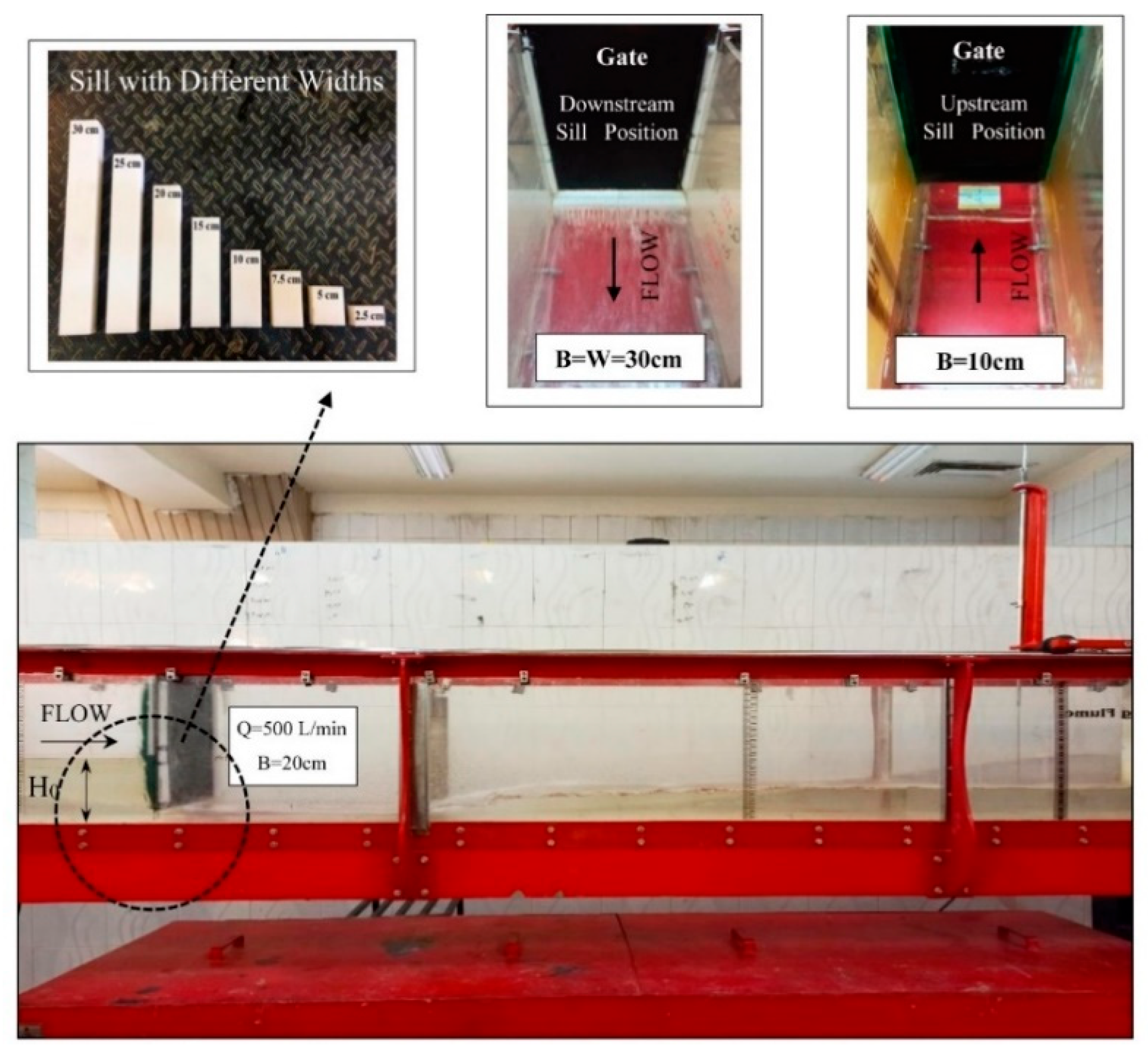
Figure 3.
Schematic view of the gate (a) no-sill case; (b) with the non-suppressed and suppressed sill in various positions; 1, 3: upward and downward tangent gate positions; 2: under gate position.
Figure 3.
Schematic view of the gate (a) no-sill case; (b) with the non-suppressed and suppressed sill in various positions; 1, 3: upward and downward tangent gate positions; 2: under gate position.
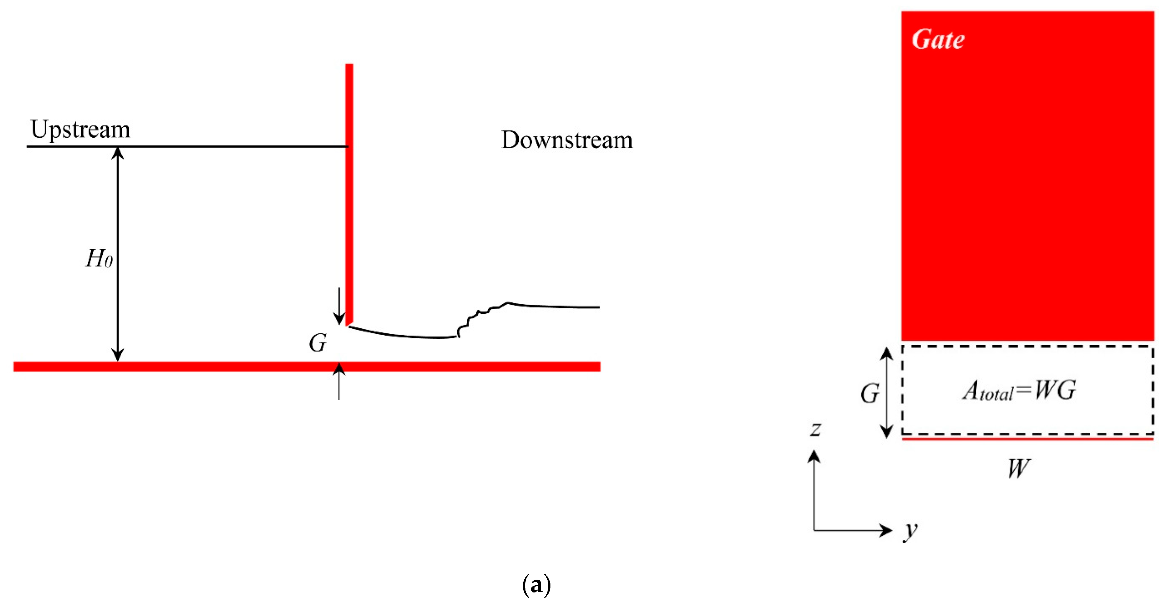
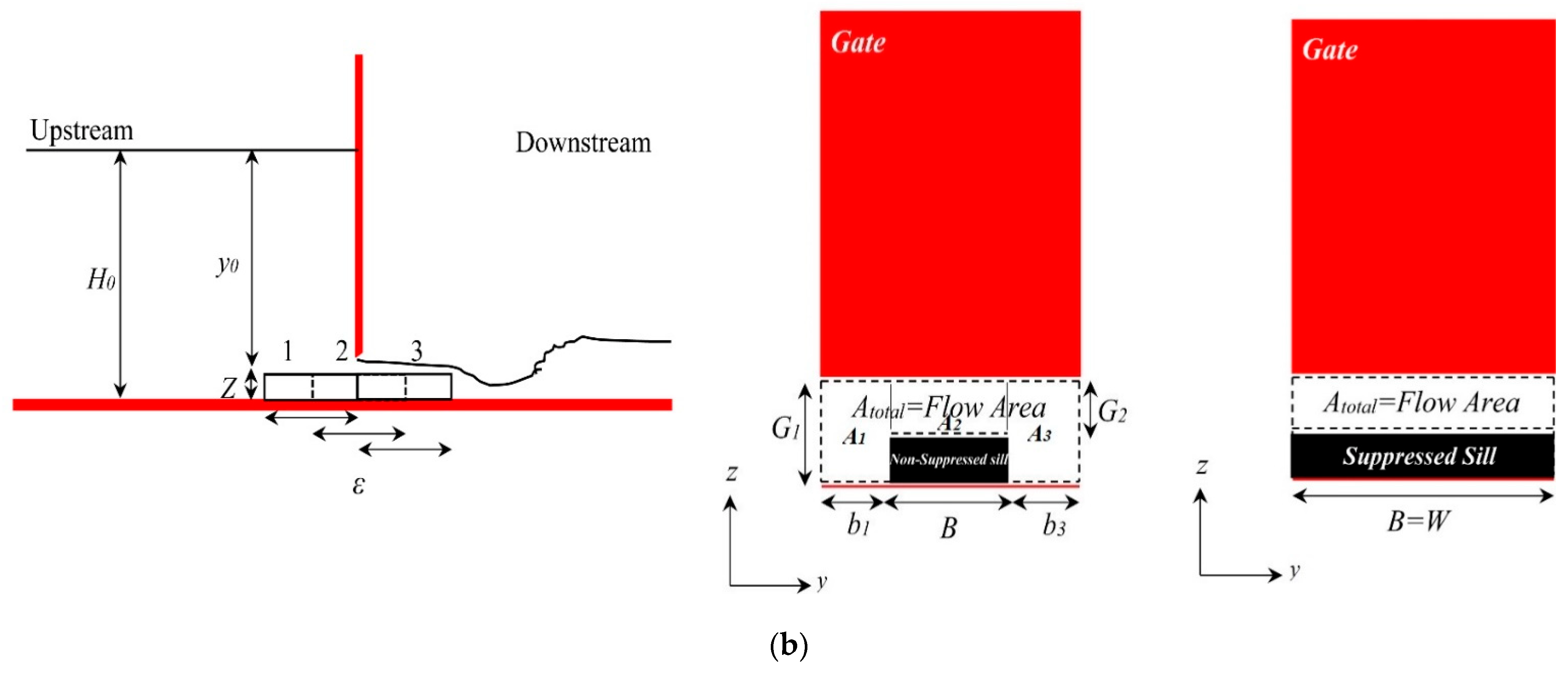
Figure 4.
3D geometry and mesh grid of model.

Figure 5.
Discharge–time hydrograph diagram.
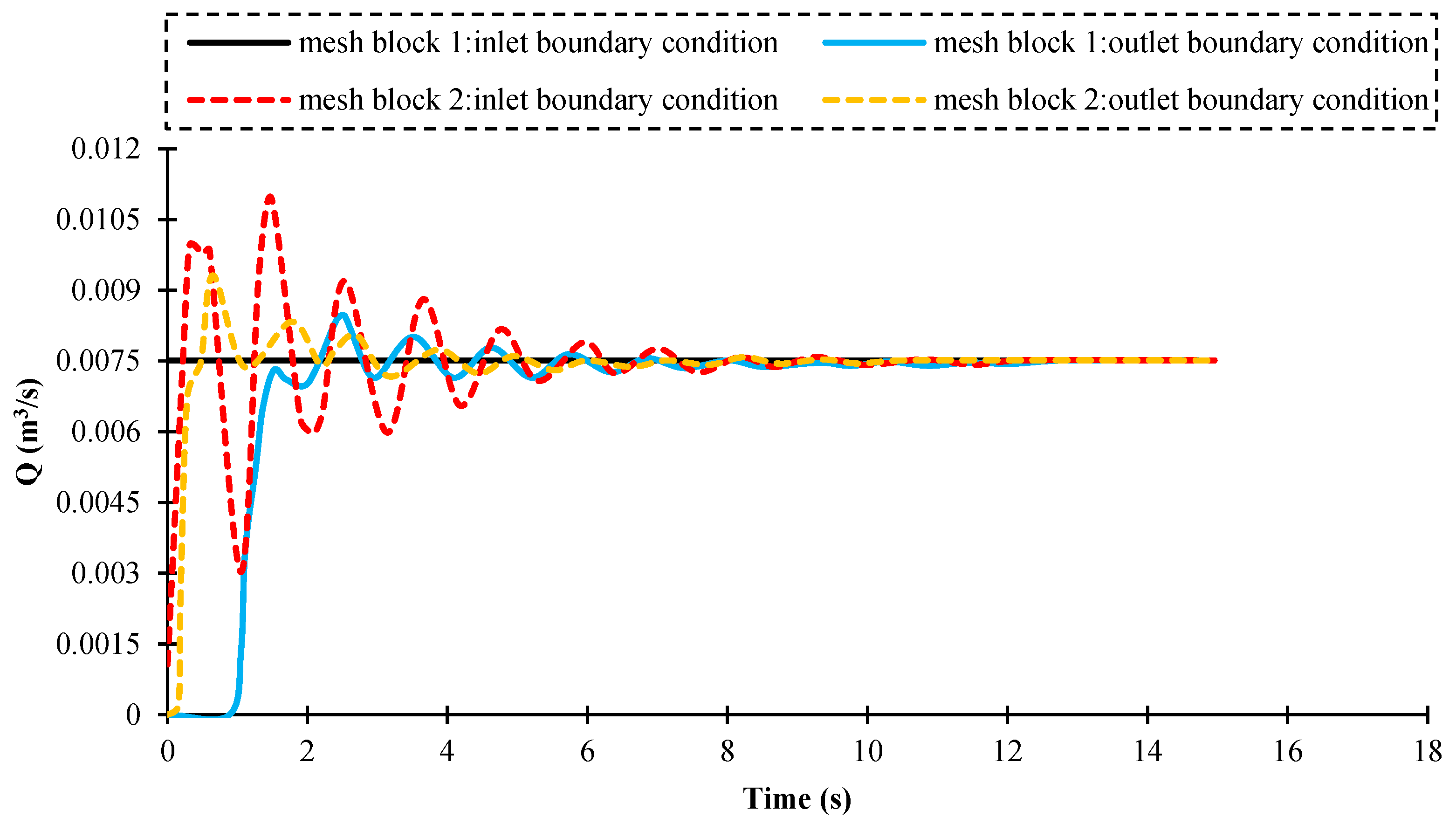
Figure 6.
Comparison of numerical solution results with experimental results: (a) data scatters; (b) longitudinal flow profile.
Figure 6.
Comparison of numerical solution results with experimental results: (a) data scatters; (b) longitudinal flow profile.

Figure 7.
(a) Changes in discharge coefficient; (b) stage–discharge for different gate openings in the no-sill state.
Figure 7.
(a) Changes in discharge coefficient; (b) stage–discharge for different gate openings in the no-sill state.
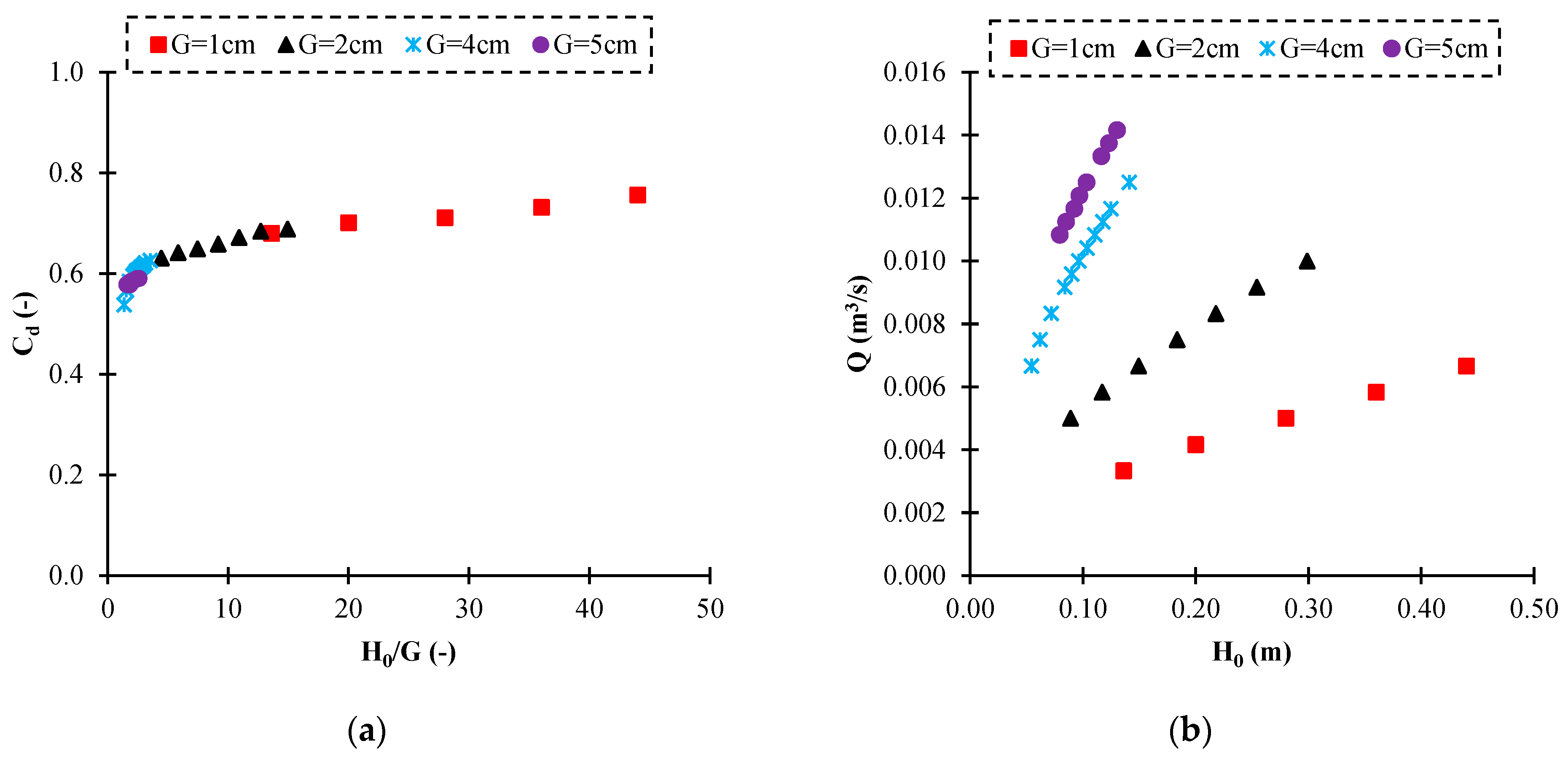
Figure 8.
Changes of discharge coefficient in different positions of the sill: (a,d) under gate position; (b,e) downward tangent gate position; (c,f) upward tangent gate position, in various gate opening.
Figure 8.
Changes of discharge coefficient in different positions of the sill: (a,d) under gate position; (b,e) downward tangent gate position; (c,f) upward tangent gate position, in various gate opening.

Figure 9.
Effect of gate opening with sill state on discharge coefficient.

Figure 10.
Comparison of discharge coefficient between the no-sill and suppressed sill states: (a) 1 cm opening; (b) 2 cm opening.
Figure 10.
Comparison of discharge coefficient between the no-sill and suppressed sill states: (a) 1 cm opening; (b) 2 cm opening.

Figure 11.
Outlet flow through the gate with different positions of the suppressed sill.
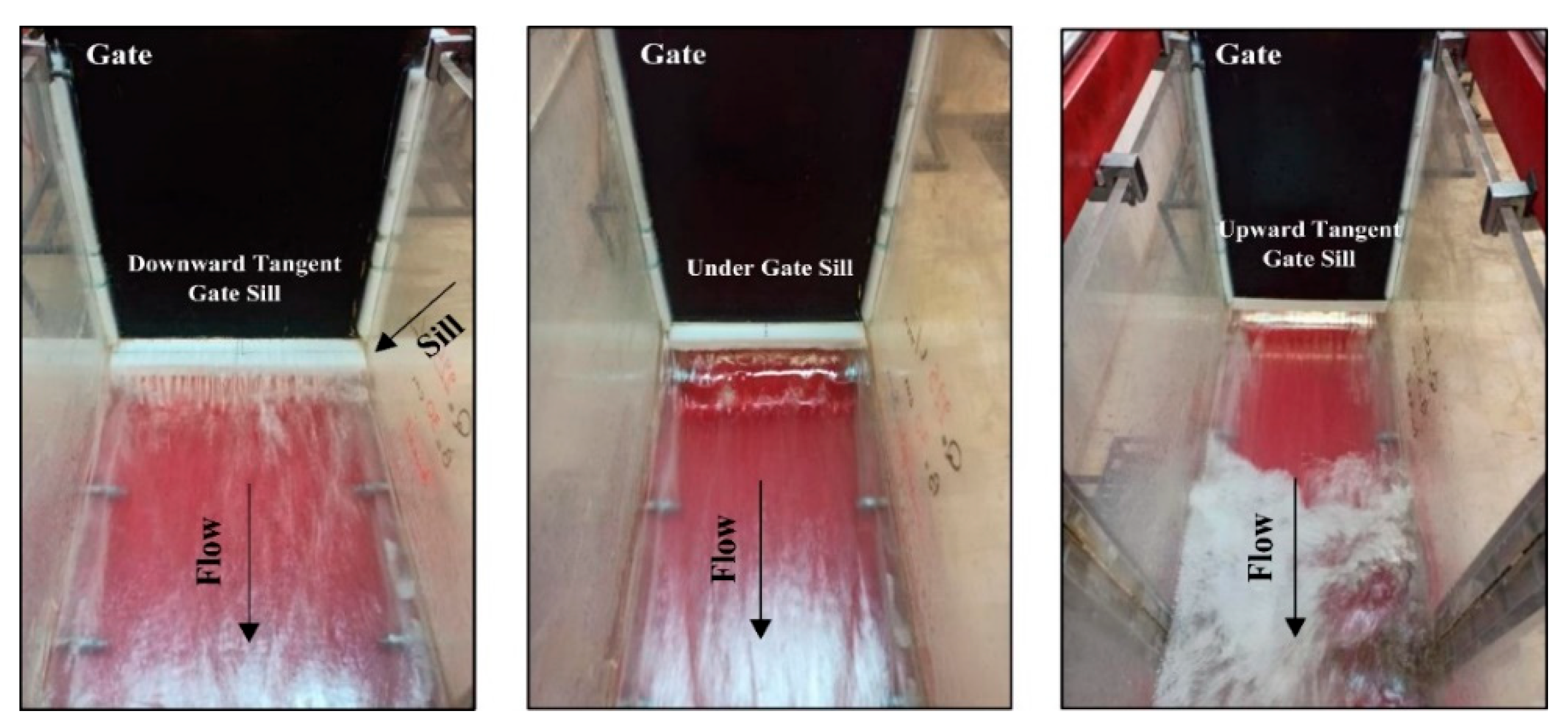
Figure 12.
Distribution of average flow velocity along the channel length in the cross-section behind the gate at the sill with thicknesses of (a) 0.05 m; (b) 0.15 m; (c) 0.25 m.
Figure 12.
Distribution of average flow velocity along the channel length in the cross-section behind the gate at the sill with thicknesses of (a) 0.05 m; (b) 0.15 m; (c) 0.25 m.
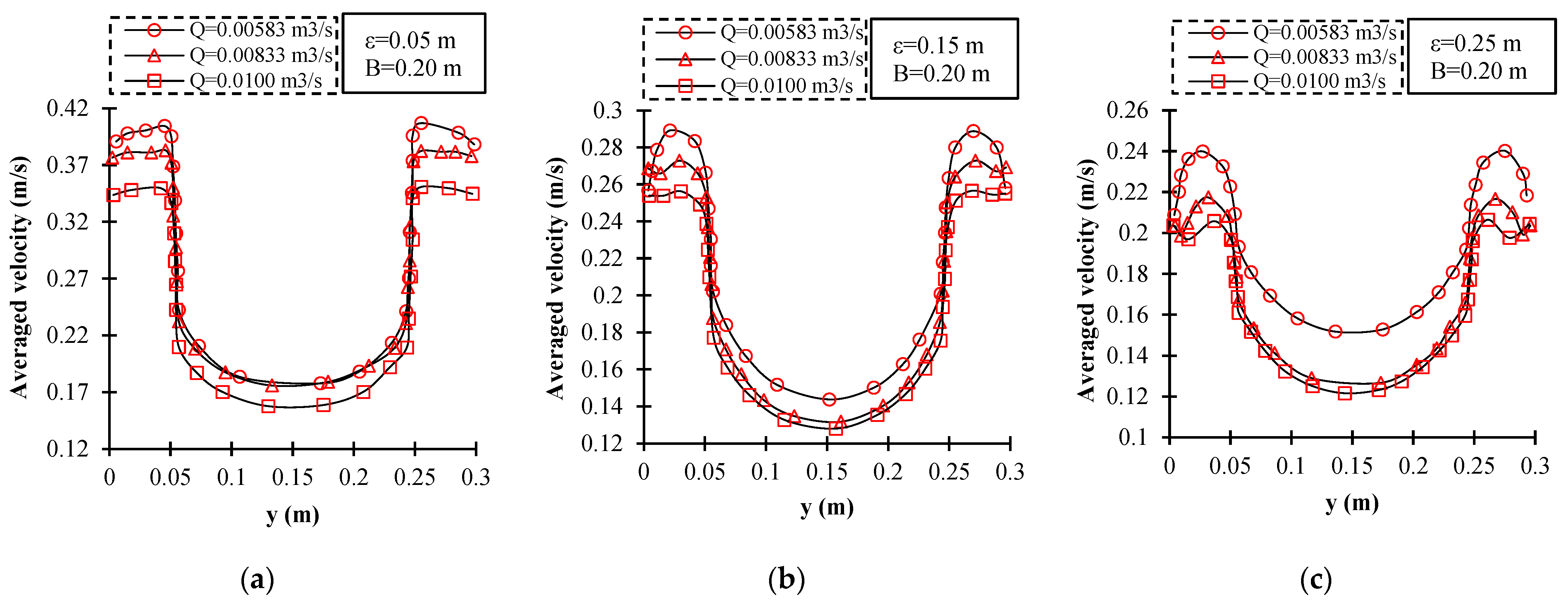
Figure 13.
Schematic view (section x–y) of shear stress at the sill with different thicknesses of (a) 0.25 m (b) 0.15 m. (c) Diagram of shear stress along the sill thickness.
Figure 13.
Schematic view (section x–y) of shear stress at the sill with different thicknesses of (a) 0.25 m (b) 0.15 m. (c) Diagram of shear stress along the sill thickness.

Figure 14.
Discharge coefficient of the gate in different thicknesses of sill (a) non-suppressed (b) suppressed.
Figure 14.
Discharge coefficient of the gate in different thicknesses of sill (a) non-suppressed (b) suppressed.
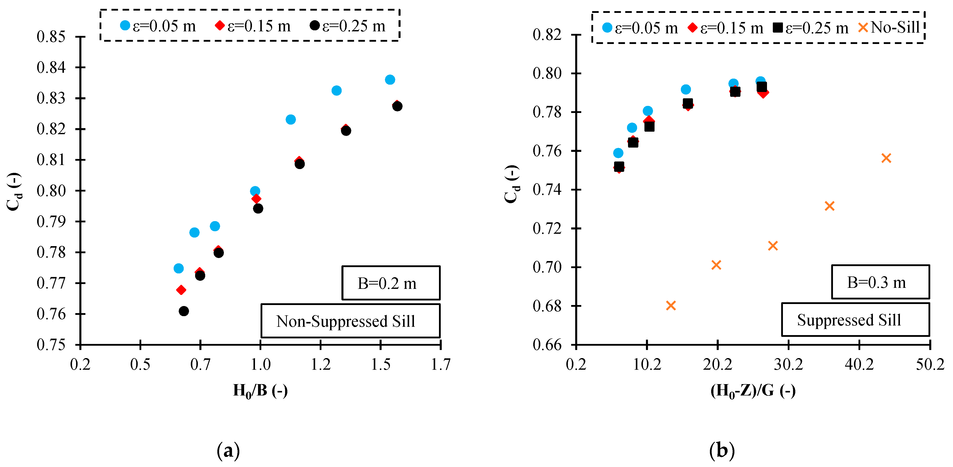
Figure 15.
(a) Effect of sill height on discharge coefficient; (b) effect ratio of sill height to gate opening on discharge coefficient.
Figure 15.
(a) Effect of sill height on discharge coefficient; (b) effect ratio of sill height to gate opening on discharge coefficient.

Figure 16.
Effect of sill height on pressure distribution on the gate.


Table 1.
Hydraulic and geometric characteristics of the studied models.
| Hydraulic Characteristics | ||||
| Q (L/min) | Upstream Water Depth (m) | Froude Number (-) | Reynolds Number (-) | |
| 150–850 | 0.05–0.44 | 0.024–0.515 | 11,111–47,222 | |
| Geometric Characteristics | ||||
| Gate opening | Sill height (m) | Sill length (m) | Sill width (m) | Sill position |
| 0.01–0.02 0.04–0.05 | 0.03–0.06–0.09 | 0.05–0.15–0.25 | 0.025–0.05–0.075–0.10 0.15–0.20–0.25–0.30 | Under gate, upward, and downward tangent gate positions |
Table 2.
Validation of the model.
| Test No. | Size of Cells (m) | Assumed Turbulence Model | Mean RE% | RMSE | KGE | |||
|---|---|---|---|---|---|---|---|---|
| H0 | Cd | H0 (m) | Cd (-) | H0 (m) | Cd (-) | |||
| 1 | Mesh block 1: 0.014 Mesh block 2: 0.007 | RNG | 14.12 | 9.28 | 0.0735 | 0.0914 | good | good |
| 2 | Mesh block 1: 0.013 Mesh block 2: 0.0065 | 6.35 | 5.72 | 0.0285 | 0.0348 | Very good | Very good | |
| 3 | Mesh block 1: 0.012 Mesh block 2: 0.007 | 3.9 | 2.95 | 0.0185 | 0.0245 | Very good | Very good | |
| 4 | Mesh block 1: 0.012 Mesh block 2: 0.006 | 2.94 | 1.60 | 0.0079 | 0.0117 | Very good | Very good | |
| 5 | Mesh block 1: 0.010 Mesh block 2: 0.005 | 2.86 | 1.50 | 0.0076 | 0.0114 | Very good | Very good | |
Table 3.
Selecting the optimal turbulence model.
| Optimal Mesh Size | Turbulence Models | RMSE | |
|---|---|---|---|
| H0 (m) | Cd (-) | ||
| Test No. 4 | RNG | 0.0079 | 0.0117 |
| k-ε | 0.0085 | 0.0123 | |
| k-ω | 0.0094 | 0.0128 | |
| LES | 0.0083 | 0.0120 | |
Table 4.
Comparison of numerical solution results with experimental results.
| Q (m3/s) | Cd (-) Exp | Cd (-) Num | RE (%) | H0 (m) Exp | H0 (m) Num | RE (%) |
|---|---|---|---|---|---|---|
| 0.00583 | 0.6515 | 0.6575 | 0.93 | 0.124 | 0.122 | 1.67 |
| 0.00625 | 0.6538 | 0.6661 | 1.89 | 0.140 | 0.135 | 3.39 |
| 0.00750 | 0.6625 | 0.6743 | 1.77 | 0.192 | 0.185 | 3.27 |
| 0.00833 | 0.6786 | 0.6927 | 2.09 | 0.224 | 0.215 | 3.86 |
| 0.00917 | 0.6823 | 0.6995 | 2.53 | 0.266 | 0.253 | 4.68 |
| 0.01000 | 0.6865 | 0.7016 | 2.16 | 0.311 | 0.298 | 4.10 |
| 0.01042 | 0.6877 | 0.6845 | 0.46 | 0.335 | 0.338 | 0.90 |
| 0.01083 | 0.6862 | 0.6921 | 0.86 | 0.363 | 0.357 | 1.65 |
Publisher’s Note: MDPI stays neutral with regard to jurisdictional claims in published maps and institutional affiliations. |
© 2022 by the authors. Licensee MDPI, Basel, Switzerland. This article is an open access article distributed under the terms and conditions of the Creative Commons Attribution (CC BY) license (https://creativecommons.org/licenses/by/4.0/).
Share and Cite
MDPI and ACS Style
Daneshfaraz, R.; Norouzi, R.; Abbaszadeh, H.; Kuriqi, A.; Di Francesco, S. Influence of Sill on the Hydraulic Regime in Sluice Gates: An Experimental and Numerical Analysis. Fluids 2022, 7, 244. https://doi.org/10.3390/fluids7070244
AMA Style
Daneshfaraz R, Norouzi R, Abbaszadeh H, Kuriqi A, Di Francesco S. Influence of Sill on the Hydraulic Regime in Sluice Gates: An Experimental and Numerical Analysis. Fluids. 2022; 7(7):244. https://doi.org/10.3390/fluids7070244
Chicago/Turabian StyleDaneshfaraz, Rasoul, Reza Norouzi, Hamidreza Abbaszadeh, Alban Kuriqi, and Silvia Di Francesco. 2022. "Influence of Sill on the Hydraulic Regime in Sluice Gates: An Experimental and Numerical Analysis" Fluids 7, no. 7: 244. https://doi.org/10.3390/fluids7070244