
Taichi-LBM3D: A Single-Phase and Multiphase Lattice Boltzmann Solver on Cross-Platform Multicore CPU/GPUs


1
Geoscience Research Centre, TOTAL E&P UK Limited, Westhill, Aberdeenshire AB32 6JZ, UK
2
Taichi Graphics, Beijing 100089, China
3
Division of Energy and Sustainability, Cranfield University, Bedford MK43 0AL, UK
*
Author to whom correspondence should be addressed.
Fluids 2022, 7(8), 270; https://doi.org/10.3390/fluids7080270
Submission received: 4 July 2022
/
Revised: 24 July 2022
/
Accepted: 3 August 2022
/
Published: 8 August 2022
Abstract
:The success of the lattice Boltzmann method requires efficient parallel programming and computing power. Here, we present a new lattice Boltzmann solver implemented in Taichi programming language, named Taichi-LBM3D. It can be employed on cross-platform shared-memory many-core CPUs or massively parallel GPUs (OpenGL and CUDA). Taichi-LBM3D includes the single- and two-phase porous medium flow simulation with a D3Q19 lattice model, Multi-Relaxation-Time (MRT) collision scheme and sparse data storage. It is open source, intuitive to understand, and easily extensible for scientists and researchers.
1. Introduction
The study of fluid flows is an important subject of civil, mechanical, and chemical engineering. Accurate calculation of the forces, pressure, and velocity can help us to better understand the flow and its mass/heat transport process. The lattice Boltzmann method (LBM) is a numerical method for simulating fluid dynamics introduced three decades ago [1,2]. Since then, it has quickly developed and has attracted significant attention in academia and industry. The lattice Boltzmann method is based on a special discretisation of velocity space, time, and space: An ensemble of particles, the motion and interactions of which are confined to a regular space–time lattice [3,4]. These particle groups are much larger than real fluid molecules, but they show the same behaviour in density and velocity as the real fluid at macroscopic scale. The Navier–Stokes equations can be recovered by LBM at macroscopic scale [5,6,7]. This unique mesoscale feature allows the LBM to simulate fluid/gas flow without directly solving continuum equations and distinguishes it from conventional computational fluid dynamics (CFD) methods: the conventional CFD method discretises the governing equation in a top-down approach, the LBM recovers the governing equations from the defined rules for discretised models in a bottom-up approach.
Several lattice models have been proposed for the LB method [6,8,9,10]. The most popular and widely used lattice model has been used in 2D and 3D [10] called D3Q19. The model contains 19 velocities at each lattice node. We used this lattice model as our LB solver implementation. The collision term is the key component in the LB method; it defines how particle groups exchange momentum and energy locally at lattice nodes. The simplest one that can be used for flow simulation is the Bhatnagar–Gross–Krook (BGK) operator [11]. A multiple-relaxation-time (MRT) scheme was developed to overcome the drawbacks of the BGK model, e.g., numerical instability [12]. Using various relaxation-time parameters for different moments of macroscopic quantities is the main concept behind MRT. The MRT approach can increase the numerical stability while lowering the computational time by at least one order of magnitude and keeping the same accuracy. A thorough analysis of MRT’s numerical stability was conducted in [13]. We used the MRT scheme as a collision term in our single- and two-phase solver development.
The LB method can be easily extended to multiphase multi-physics applications due to its mesoscopic nature. There have been many multiphase/multicomponent LB models proposed in the past two decades. These models generally can be grouped into four categories: the colour gradient model [14,15,16,17,18], the free energy model [19,20,21], the pseudo-potential Shan–Chen model [22,23,24,25], and the phase-field model [26,27,28]. We implemented an optimised colour-gradient model proposed in [18], which permits improved numerical stability, a higher viscosity ratio, and a lower capillary number compared to other two-phase models.
Compared with conventional CFD techniques, the LBM has several advantages:
- -
- It is relatively simple to implement. LBM relies on particle group distributions. The interaction between nodes are fully linear, while the nonlinearity enters into a local collision process within each node [29]
- -
- The LBM algorithm is mostly local, leading to efficiency and scalability on a parallel computer [30]
- -
- Robust handling of complex geometries.
In the past few decades, several code packages emerged and have been well-maintained, including Palabos [31], OpenLB [32], Walbera [33], and many others [34]. Most of them were implemented in C++ on CPU architecture for its high computing efficiency and object-oriented language. However, the parallel packages require strong programming skills, e.g., CUDA and C++. To remove these barriers and allow the researcher to focus on algorithm and application development, we developed a 3D single-phase MRT LBM solver and two-phase improved colour gradient MRT solver [18] using Taichi programming languages [35], named Taichi-LBM3D. The objective of this new LBM solver is to facilitate researchers who want to focus on the LB algorithm or application but not on the programming, while guaranteeing the high computing efficiency on parallel platforms. The researchers could prototype their new algorithm rapidly and/or test their new applications on multicore CPUs or massively parallel GPUs. Interestingly enough, recent efforts were found to use PyTorch [36] to develop LBM models on GPUs, but these were limited to single-phase flow applications.
Based on the Taichi computing infrastructure, Taichi-LBM3D can be executed on a shared memory cross-platform with CPU backend (e.g., x86, ARM64) and GPUs (CUDA, Metal and OpenGL). The implementation is short: Around 400 lines for single-phase flow and 500 lines for two-phase flow. The solver is also intuitive to understand and is implemented using python-like syntax along with Taichi embedded vector/matrix operations. This unique feature allows further extension with minimum effort. In addition, the solver has a sparse storage option, which is essential for the simulation of flow over a porous medium. The sparse storage option is decoupled from the computing kernel. The computing performance is comparable with original C++ implementation on CPUs and much faster on GPUs. Researchers will be able to test new ideas and applications on Taichi-LBM3D without losing computing efficiency, and development time can be potentially reduced from days to hours. Taichi-LBM3D would enable integrating the LBM simulations with Taichi’s automatic differentiation facility [37], which will be our future work. This paper is organised as follows. Section 2 presents the overview of the LBM algorithm and its implementation. Section 3 shows three benchmark problems for the Stokes flow, Navier–Stokes flow, and the two-phase flow. Section 4 shows different numerical applications and the overall speed comparison. Section 5 presents a summary and conclusion.
2. Algorithm
The lattice Boltzmann method (LBM) uses a discrete Boltzmann equation to simulate fluid flow that divides the algorithm into a collision and a streaming step. The location of the particle distribution functions (PDFs) in space is presented on the nodes of the lattice grid, and a small set of lattice velocities are used to represent the particle velocities. Under the assumption of a low Mach number , the Maxwell–Boltzmann distribution can resemble the equilibrium to second-order accuracy in velocity. To implement a lattice Boltzmann simulation, four major steps should be included:
- Initialisation of the distribution function
- Collision step: A time iteration takes the populations from their state at time t to the next state , where is a constant discrete time step:
We used the multi-relaxation-time scheme D3Q19 lattice Boltzmann method for the Stokes flow calculation [13], which allows independent adjust adjustment of the bulk and shear viscosity, which significantly improves the numerical stability for a low viscosity fluid. D3 represents the space dimension and Q19 indicates the number of discretised microscopic velocities, where is the discretised microscopic velocities:
where , is the lattice length, and is the constant time step. The weights for the D3Q19 stencil are
The multi-relaxation-time (MRT) collision operator is:
The collision process is conducted in the momentum space, and the equilibrium moment is calculated by . The moments of the distribution function are expressed as
The physical meaning of these moments can be found in [12]. The collision diagonal matrix is a diagonal comprised of relaxation rates:
The relaxation rates and are associated with the kinematic viscosity and bulk viscosity , respectively, that can be calculated as:
The relaxation time is defined as . We chose the following value
- 3.
- Streaming step:Different boundary conditions, e.g., simple bounce-back and periodic, were implemented.
- 4.
- Computation of macroscopic hydrodynamic quantities, density, and momentum are conserved values that can be calculated from:
Multicomponent Lattice Boltzmann Models
A general colour gradient lattice Boltzmann model can be summarised in 4 steps
- Single phase collision using MRT scheme
- Surface tension perturbation to obtaining
- Recolouring
- Streaming.
We employed an optimised colour-gradient approach [18] for the two-phase flow problem. To maintain the inbuilt parallelism of the lattice Boltzmann method, only the values of distribution functions of the nearest neighbour nodes were required. High viscosity ratios and a low capillary number problem were possible in this model, as it increased numerical stability. Velocity and pressure use only one full size distribution function. A recolouring approach was used to limit the diffusion on the interface while adding additional terms to the equilibrium moments in the MRT collision stage. Two component densities were indicated by the variables and . The definition of parameter is
The colour gradient vector of the phase field can be calculated using
The orientation of the interface can be obtained by a normalised gradient:
The two separate LB equations will compute the convection of density field , . Take for example,
The equilibrium distribution function is
Only the local equilibrium distribution function is required in the collision step. Thus, only the summation needs to be recorded rather than all the values.
The gradient of the phase field is required to calculate the surface tension term. The extra terms for the surface tension are
The relaxation matrix, kinematic, and bulk viscosity calculation are the same as a standard MRT–LBM.
The Taichi-LBM3D scripts are easy to understand and can be easily modified by the users. For example, the collision operator in Equation (4) is the most computation intensive task in the LBM algorithm. The reader could easily refer to Listing 1 and Equation (4). Another benefit is the sparse data structure that has been built in Taichi. Listing 2 shows the dense and sparse memory allocation in Taichi.
| Listing 1. Example of collision operator in Taichi-LBM3D for single phase flow problem. |
 |
| Listing 2. Examples of dense and sparse memory allocation in Taichi-LBM3D. |
 |
3. Numerical Benchmark
In this section, the implementation of the Taichi-LBM3D is benchmarked by comparison with well-known numerical test cases. We started with the viscous-driven to inertia-driven flow; finally, we benchmarked the two-phase capillary fingering.
3.1. Stokes Flow
Here, we considered a Plane Poiseuille flow problem. The flow was created between two infinitely long parallel plates. A constant pressure gradient was applied in the direction of flow. The analytical velocity profile is described by the Poiseuille equation
where f is the pressure gradient or a body force, x is the coordinate, is the viscosity, and is the distance between two plates. We chose four different widths 3, 5, 11, and 21 lattice points. The comparison of the simulated results and analytical results are shown in Figure 1. Excellent agreement was achieved for all widths, due to the use of halfway bounce-back boundary conditions for the walls along the flow direction and the usage of the multiple-relaxation-time scheme.
3.2. Lid-Driven Flow
The 3D lid-driven flow is a classic benchmark problem and has been extensively validated [38,39], especially for laminar flow cases. The flow in a cube chamber was driven by a constant velocity at the top lid. The domain was . The top wall had a velocity (1,0,0). The laminar flow with Reynolds number was considered for our benchmark. The flow will become steady state at , and the simulation was performed until the relative residual reached the tolerance. Figure 2 shows a comparison of velocity profiles through the centre of the cavity with a lattice refinement of , , , and . It can be observed that the simulated results agreed with the references with mesh refinement [38]. The iso-surfaces of the Q-criterion of the velocity field for the lattice size are shown in Figure 2.
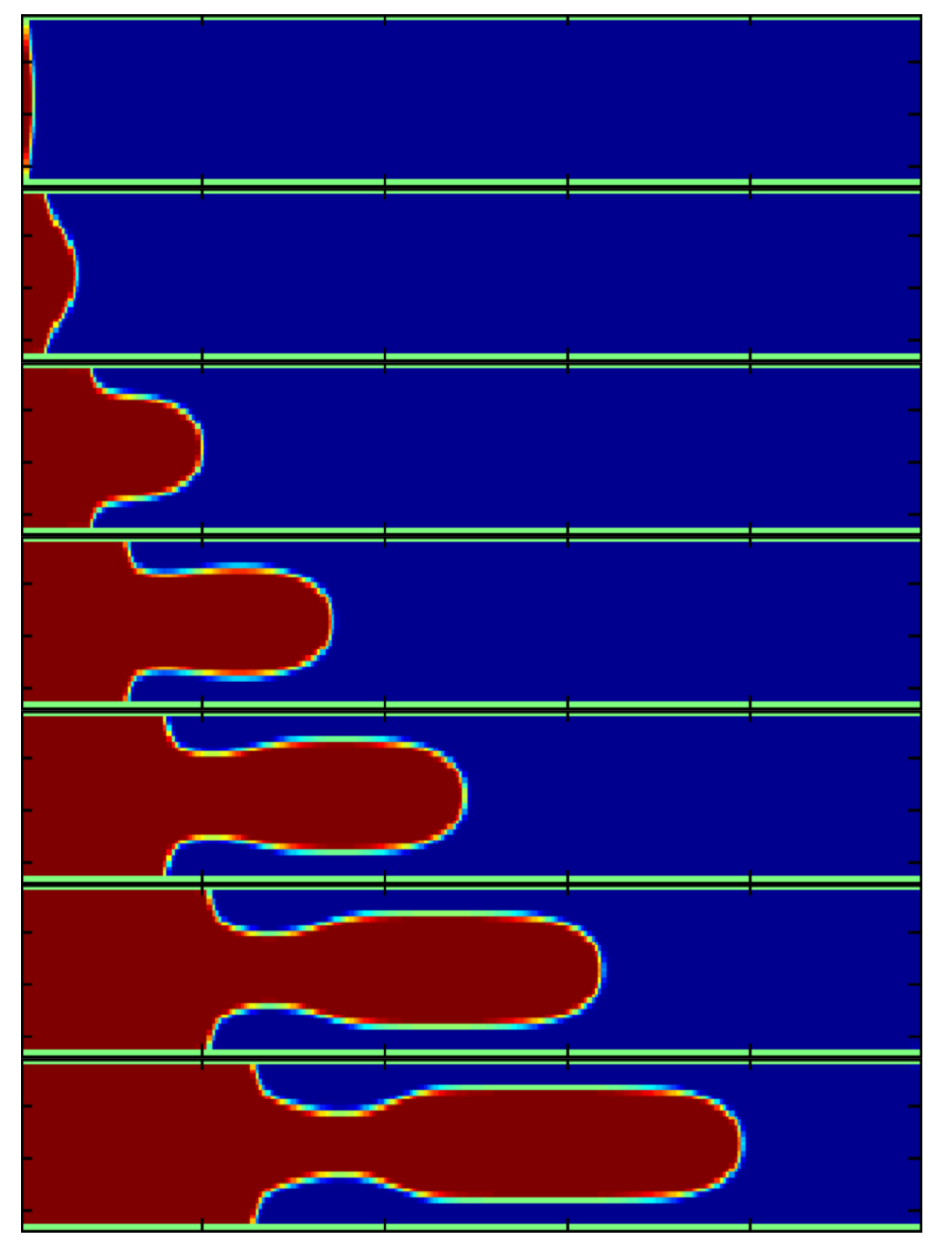
3.3. Capillary Fingering
Capillary fingering is a well-known hydrodynamic instability problem, and it was used to validate the LBM multicomponent model. Two fluids had different viscosities. One fluid was displaced by a second phase of fluid along a non-slip channel. A growing finger of the driving fluid was observed if the capillary number was large enough. The is defined as
where is the velocity of the tip of finger, is the kinematic viscosity of the driving fluids, and is the surface tension. The colour gradient model was used to study the capillary fingering. A lattice size 512 × 32 was used. The first half of the domain contained substance 0, and the rest was occupied by phase 1. Periodic boundary conditions were used in the x direction and bounded with non-slip boundaries. A pressure gradient was imposed by applying a body force in the x direction. Figure 3 shows the evolution of fingers for binary fluids with a viscosity ratio of 20 and a tip velocity of 0.05 simulated by the colour gradient model. Halpern and Gaver [40] studied the fingering phenomenon in a channel, by measuring the width of the fingers as a function of the capillary number . The simulated results with the colour gradient models were compared with reference [40], as shown in Figure 4. A good agreement with the experimental data can be seen. These numerical examples show that the fingering phenomena can be captured and properly modelled in Taichi-LBM3D.
4. Engineering Applications
This section presents a list of numerical applications from inertia dominated flow to viscous dominated flow and from single phase to two phase to illustrate the wide range of Taichi-LBM3D capability.
4.1. Single Phase Flow
In this section, an inertia-dominated external flow problem with direct numerical simulation is presented. The geometry is from a car and an urban building model. The 3D CAD models were first converted into voxel-based images, by a binary matrix with 0 and 1 that represented pore nodes and solids, respectively. There are many voxelisation tools available [41,42]. A uniform flow condition was imposed with a grid of and for these two cases. The streamlines were plotted in Figure 5. The second order accurate halfway bounce-back boundary condition was used. There was no turbulence model for all the simulations.
4.2. Simulation of Single-Phase Flow in Porous Media with Sparse Data Storage
Here, we validated the Taichi-LBM3D solver for porous media application and compared the permeability with the standard CPU implementation. A porous medium with a Fontainebleau sandstone was extracted from the image of a cylindrical core [43,44]. Here, we tested the Fontainebleau sandstone sample with a resolution of 7.5 (μm/pixel) with porosity 13%. The flow was driven only by a body force. The flow field of porous medium flow is shown in Figure 6. The permeability of a porous medium can be calculated from the empirical Darcy’s law. We reached the same permeability value with 789 (mD) with the flow resolution , with a sparse storage scheme, which significantly reduced the memory requirement in proportion to the porosity.
4.3. Two-Phase Flow with Sparse Data Storage for Porous Medium
A two-phase flow through the same Fontainebleau sandstone is presented in this case. To simulate the drainage and imbibition processes, two buffer layers were added at the inlet and outlet of the sample to allow fluid to be injected and flow out. The contact angle of the solid surface was specified as = 0.7; this value is the cosine of the desired contact angle, and the value is between −1 and 1. The interfacial tension of the two phases was set at .
Figure 7 shows the snapshots of the Bentheimer sandstone drainage process. Excluding the inlet layer, which was saturated with oil initially, the sample was completely saturated with water (wetting phase) (non-wetting phase). To drive the non-wetting fluid into the sample, the uniform body force was added in the x-direction. Before entering the inlet, the fluid that was moving out changed colour and entered a non-wetting phase. This simulated a pure injection drainage process with a non-wetting phase. Given the high capillary pressure, some small holes and throats were not filled with a non-wetting phase.
4.4. Performance Tests on Parallel Platforms
Taichi programming languages provide good performance on different platforms. The adopted computing platforms were an NVIDIA A100, AMD Radeon Pro 5300 4 GB in Metal backend, and 3.3 GHz 6-Core Intel Core i5 with 12 threads. A modified performance metric for LBM codes is Million Lattice Updates per Second (MLUPs) considering the porosity for flow over porous media. This metric is calculated by
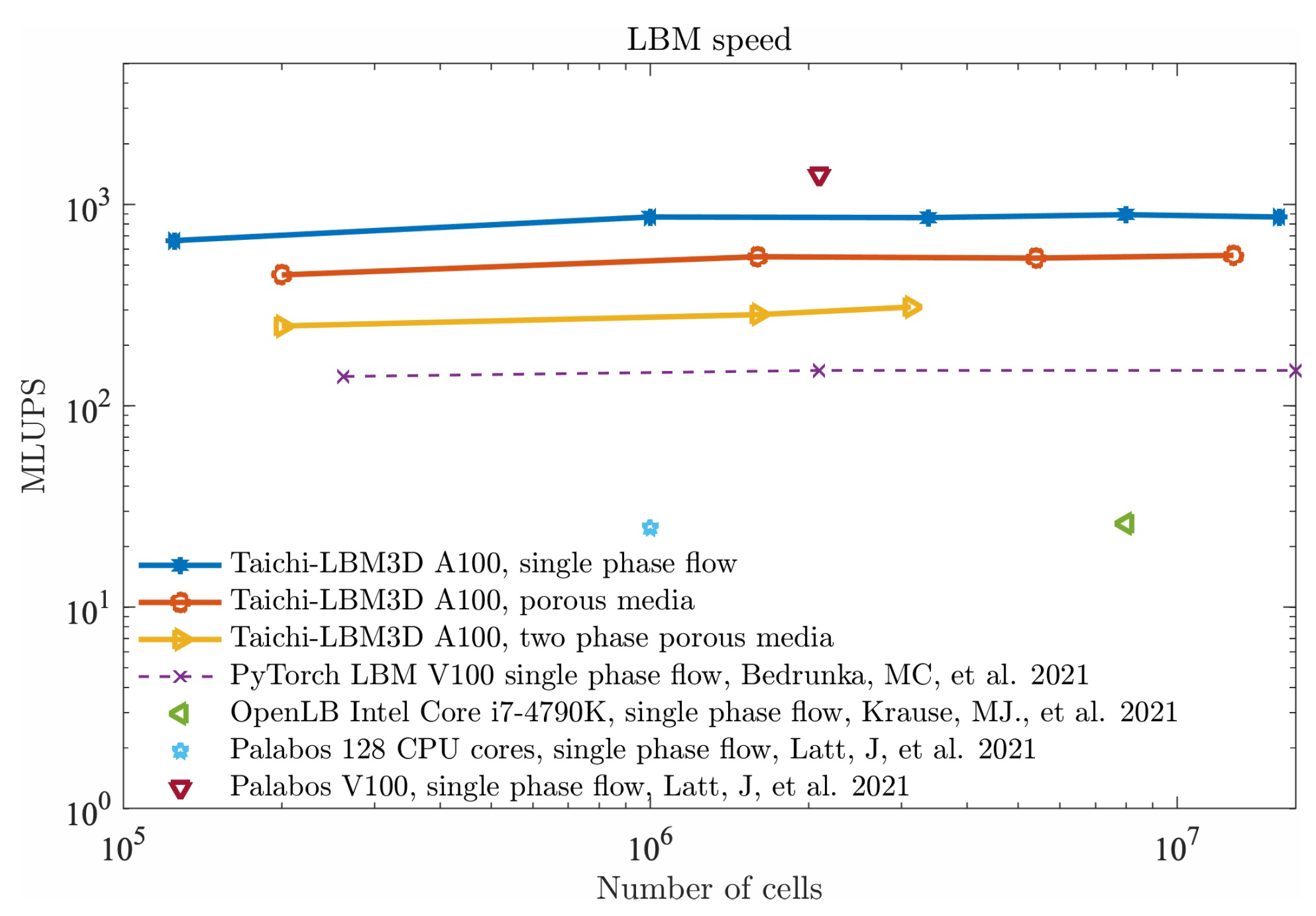
where , , and are the dimensions of the simulations. CPUs and NVIDIA A100 support both double and single precision. The AMD Radeon Pro 5300 4 GB in metal backend supports single precision only, so all the cases were shown in single precision for comparison purposes. Three flow problems were run under mesh refinement from single phase to multiphase. The details of computation speed are reported in Table 1.The computation speeds reached over 900 MLUPs using an NVIDIA A100 with D3Q19 and MRT. The performance was much better than the PyTorch implementation with 150 MLUPs reported in [36]. Other popular LBM codes, e.g., the latest version of OpenLB [32], require over 200 cores CPUs to reach the same speed. Palabos showed 24.8 MLUPS at 128 cores and required over 4000 cores to reach 900 MLUPs [31]. The current version of implementation shows that the NVIDIA A100 was 60 times faster than its CPU counterpart. Figure 8 shows the overall comparison of performance of Taichi-LBM3D with other codes reported in the literature. The implementation will require further optimisation. A well-optimised LBM algorithm could reach over 1000 MLUPs using V100 GPU [31].
5. Conclusions
In this work, we presented Taichi-LBM3D, a novel cross-platform 3D single-phase and two-phase LBM solver on shared-memory many-core CPUs or GPUs implemented in Taichi programming language. We were able to produce an LBM solver under 500 lines of code for a complex two-phase problem with surface tension. Scientists and engineers could easily prototype their LBM models and employ them on GPU-accelerated workstations. Numerical implementation was benchmarked with three well-known problems with convergence studies. A wide range of applications from viscous and capillary to inertia dominated flow was shown. In the last, the MLUPS were employed to measure the speed of LBM under different platforms. The performance of the NVIDIA A100 GPU reached over 900 MLUPS for single-phase flow and 500 for two-phase flow with surface tension. It is approximately 60 times faster than the 3.3 GHz 6-Core Intel Core i5. The code is available under MIT Licence on GitHub.
Author Contributions
Conceptualisation, J.Y. and L.Y.; methodology, J.Y., Y.X. and L.Y.; software, J.Y., Y.X. and L.Y.; validation, J.Y., Y.X. and L.Y.; formal analysis, J.Y. and L.Y.; investigation, J.Y. and L.Y.; writing, review, and editing, J.Y. and L.Y. All authors read and agreed to the published version of the manuscript.
Funding
This research was funded by Supergen ORE ECR Fund and British Council.
Data Availability Statement
The Taichi-LBM3D is open source under MIT License and available in the Github repository at https://github.com/yjhp1016/taichi_LBM3D (accessed on 1 February 2022).
Acknowledgments
The authors acknowledge the support from the Taichi developer community and the Delta 2 HPC facility at Cranfield University. L. Yang acknowledges the support from EPSRC Supergen ORE ECR Fund, “Parametric study for flapping foil system for harnessing wave energy”.
Conflicts of Interest
The authors declare no conflict of interest.
Abbreviations
The following abbreviations are used in this manuscript:
| CPU | Central processing unit |
| GPU | Graphics processing unit |
| CFD | Computational fluid dynamics |
| BGK | Bhatnagar–Gross–Krook |
| OpenGL | Open Graphics Library |
| CUDA | Compute unified device architecture |
| LBM | Lattice Boltzmann method |
| HPC | High performance computing |
| MRT | Multiple-relaxation-time |
| MLUPS | Million lattice updates per second |
| D3Q19 | Three-dimensional lattice stencil with 19 discrete velocity directions in each node |
References
- Higuera, F.J.; Jiménez, J. Boltzmann approach to lattice gas simulations. EPL Europhys. Lett. 1989, 9, 663. [Google Scholar] [CrossRef]
- McNamara, G.R.; Zanetti, G. Use of the Boltzmann equation to simulate lattice-gas automata. Phys. Rev. Lett. 1988, 61, 2332. [Google Scholar] [CrossRef] [PubMed]
- Benzi, R.; Succi, S.; Vergassola, M. The lattice Boltzmann equation: Theory and applications. Phys. Rep. 1992, 222, 145–197. [Google Scholar] [CrossRef]
- Chen, S.; Doolen, G.D. Lattice Boltzmann method for fluid flows. Annu. Rev. Fluid Mech. 1998, 30, 329–364. [Google Scholar] [CrossRef] [Green Version]
- Frisch, U.; Hasslacher, B.; Pomeau, Y. Lattice-gas automata for the Navier–Stokes equation. Phys. Rev. Lett. 1986, 56, 1505. [Google Scholar] [CrossRef] [Green Version]
- Chen, H.; Chen, S.; Matthaeus, W.H. Recovery of the Navier–Stokes equations using a lattice-gas Boltzmann method. Phys. Rev. A 1992, 45, R5339. [Google Scholar] [CrossRef]
- Ladd, A.J. Numerical simulations of particulate suspensions via a discretized Boltzmann equation. Part 1. Theoretical foundation. J. Fluid Mech. 1994, 271, 285–309. [Google Scholar] [CrossRef] [Green Version]
- d’Humières, D.; Lallemand, P.; Frisch, U. Lattice gas models for 3D hydrodynamics. EPL Europhys. Lett. 1986, 2, 291. [Google Scholar] [CrossRef]
- Higuera, F.; Succi, S.; Benzi, R. Lattice gas dynamics with enhanced collisions. EPL Europhys. Lett. 1989, 9, 345. [Google Scholar] [CrossRef]
- Qian, Y.H.; d’Humières, D.; Lallemand, P. Lattice BGK models for Navier–Stokes equation. EPL Europhys. Lett. 1992, 17, 479. [Google Scholar] [CrossRef]
- Bhatnagar, P.L.; Gross, E.P.; Krook, M. A model for collision processes in gases. I. Small amplitude processes in charged and neutral one-component systems. Phys. Rev. 1954, 94, 511. [Google Scholar] [CrossRef]
- d’Humières, D. Multiple–relaxation–time lattice Boltzmann models in three dimensions. Philos. Trans. R. Soc. Lond. Ser. Math. Phys. Eng. Sci. 2002, 360, 437–451. [Google Scholar] [CrossRef] [PubMed]
- Lallemand, P.; Luo, L.S. Theory of the lattice Boltzmann method: Dispersion, dissipation, isotropy, Galilean invariance, and stability. Phys. Rev. E 2000, 61, 6546. [Google Scholar] [CrossRef] [PubMed] [Green Version]
- Gunstensen, A.K.; Rothman, D.H.; Zaleski, S.; Zanetti, G. Lattice Boltzmann model of immiscible fluids. Phys. Rev. A 1991, 43, 4320. [Google Scholar] [CrossRef]
- Grunau, D.; Chen, S.; Eggert, K. A lattice Boltzmann model for multiphase fluid flows. Phys. Fluids A Fluid Dyn. 1993, 5, 2557–2562. [Google Scholar] [CrossRef] [Green Version]
- Lishchuk, S.; Care, C.; Halliday, I. Lattice Boltzmann algorithm for surface tension with greatly reduced microcurrents. Phys. Rev. E 2003, 67, 036701. [Google Scholar] [CrossRef]
- Latva-Kokko, M.; Rothman, D.H. Diffusion properties of gradient-based lattice Boltzmann models of immiscible fluids. Phys. Rev. E 2005, 71, 056702. [Google Scholar] [CrossRef]
- Ahrenholz, B.; Tölke, J.; Lehmann, P.; Peters, A.; Kaestner, A.; Krafczyk, M.; Durner, W. Prediction of capillary hysteresis in a porous material using lattice-Boltzmann methods and comparison to experimental data and a morphological pore network model. Adv. Water Resour. 2008, 31, 1151–1173. [Google Scholar] [CrossRef]
- Swift, M.R.; Osborn, W.; Yeomans, J. Lattice Boltzmann simulation of nonideal fluids. Phys. Rev. Lett. 1995, 75, 830. [Google Scholar] [CrossRef] [Green Version]
- Swift, M.R.; Orlandini, E.; Osborn, W.; Yeomans, J. Lattice Boltzmann simulations of liquid-gas and binary fluid systems. Phys. Rev. E 1996, 54, 5041. [Google Scholar] [CrossRef]
- Inamuro, T.; Konishi, N.; Ogino, F. A Galilean invariant model of the lattice Boltzmann method for multiphase fluid flows using free-energy approach. Comput. Phys. Commun. 2000, 129, 32–45. [Google Scholar] [CrossRef]
- Shan, X.; Chen, H. Lattice Boltzmann model for simulating flows with multiple phases and components. Phys. Rev. E 1993, 47, 1815. [Google Scholar] [CrossRef] [PubMed] [Green Version]
- Shan, X.; Chen, H. Simulation of nonideal gases and liquid-gas phase transitions by the lattice Boltzmann equation. Phys. Rev. E 1994, 49, 2941. [Google Scholar] [CrossRef] [PubMed] [Green Version]
- Sbragaglia, M.; Benzi, R.; Biferale, L.; Succi, S.; Sugiyama, K.; Toschi, F. Generalized lattice Boltzmann method with multirange pseudopotential. Phys. Rev. E 2007, 75, 026702. [Google Scholar] [CrossRef] [Green Version]
- Li, Q.; Luo, K.; Li, X. Lattice Boltzmann modeling of multiphase flows at large density ratio with an improved pseudopotential model. Phys. Rev. E 2013, 87, 053301. [Google Scholar] [CrossRef] [Green Version]
- He, X.; Chen, S.; Zhang, R. A lattice Boltzmann scheme for incompressible multiphase flow and its application in simulation of Rayleigh–Taylor instability. J. Comput. Phys. 1999, 152, 642–663. [Google Scholar] [CrossRef]
- Inamuro, T.; Ogata, T.; Tajima, S.; Konishi, N. A lattice Boltzmann method for incompressible two-phase flows with large density differences. J. Comput. Phys. 2004, 198, 628–644. [Google Scholar] [CrossRef]
- Li, Q.; Luo, K.; Gao, Y.; He, Y. Additional interfacial force in lattice Boltzmann models for incompressible multiphase flows. Phys. Rev. E 2012, 85, 026704. [Google Scholar] [CrossRef] [Green Version]
- Krüger, T.; Kusumaatmaja, H.; Kuzmin, A.; Shardt, O.; Silva, G.; Viggen, E.M. The Lattice Boltzmann Method; Springer: Berlin/Heidelberg, Germany, 2017; Volume 10, pp. 4–15. [Google Scholar]
- Succi, S. The Lattice Boltzmann Equation: For Fluid Dynamics and Beyond; Oxford University Press: Oxford, UK, 2001. [Google Scholar]
- Latt, J.; Malaspinas, O.; Kontaxakis, D.; Parmigiani, A.; Lagrava, D.; Brogi, F.; Belgacem, M.B.; Thorimbert, Y.; Leclaire, S.; Li, S.; et al. Palabos: Parallel lattice Boltzmann solver. Comput. Math. Appl. 2021, 81, 334–350. [Google Scholar] [CrossRef]
- Krause, M.J.; Kummerländer, A.; Avis, S.J.; Kusumaatmaja, H.; Dapelo, D.; Klemens, F.; Gaedtke, M.; Hafen, N.; Mink, A.; Trunk, R.; et al. OpenLB—Open source lattice Boltzmann code. Comput. Math. Appl. 2021, 81, 258–288. [Google Scholar] [CrossRef]
- Feichtinger, C.; Götz, J.; Donath, S.; Iglberger, K.; Rüde, U. WaLBerla: Exploiting massively parallel systems for lattice Boltzmann simulations. In Parallel Computing; Springer: Berlin/Heidelberg, Germany, 2009; pp. 241–260. [Google Scholar]
- Huang, C.; Shi, B.; Guo, Z.; Chai, Z. Multi-GPU based lattice Boltzmann method for hemodynamic simulation in patient-specific cerebral aneurysm. Commun. Comput. Phys. 2015, 17, 960–974. [Google Scholar] [CrossRef]
- Hu, Y.; Li, T.M.; Anderson, L.; Ragan-Kelley, J.; Durand, F. Taichi: A language for high-performance computation on spatially sparse data structures. ACM Trans. Graph. 2019, 38, 1–16. [Google Scholar] [CrossRef] [Green Version]
- Bedrunka, M.C.; Wilde, D.; Kliemank, M.; Reith, D.; Foysi, H.; Krämer, A. Lettuce: Pytorch-based lattice boltzmann framework. In Proceedings of the International Conference on High Performance Computing; Springer: Berlin/Heidelberg, Germany, 2021; pp. 40–55. [Google Scholar]
- Hu, Y.; Anderson, L.; Li, T.M.; Sun, Q.; Carr, N.; Ragan-Kelley, J.; Durand, F. Difftaichi: Differentiable programming for physical simulation. arXiv 2019, arXiv:1910.00935. [Google Scholar]
- Yang, J.Y.; Yang, S.C.; Chen, Y.N.; Hsu, C.A. Implicit weighted ENO schemes for the three-dimensional incompressible Navier–Stokes equations. J. Comput. Phys. 1998, 146, 464–487. [Google Scholar] [CrossRef] [Green Version]
- Yang, L.; Badia, S.; Codina, R. A pseudo-compressible variational multiscale solver for turbulent incompressible flows. Comput. Mech. 2016, 58, 1051–1069. [Google Scholar] [CrossRef] [Green Version]
- Halpern, D.; Gaver, D., III. Boundary element analysis of the time-dependent motion of a semi-infinite bubble in a channel. J. Comput. Phys. 1994, 115, 366–375. [Google Scholar] [CrossRef]
- Bacciaglia, A.; Ceruti, A.; Liverani, A. A systematic review of voxelization method in additive manufacturing. Mech. Ind. 2019, 20, 630. [Google Scholar] [CrossRef] [Green Version]
- Thorpe, D.B. Cad2Vox. 2022. Available online: https://github.com/bjthorpe/Cad2vox (accessed on 1 June 2022).
- Yang, L.; Yang, J.; Boek, E.; Sakai, M.; Pain, C. Image-based simulations of absolute permeability with massively parallel pseudo-compressible stabilised finite element solver. Comput. Geosci. 2019, 23, 881–893. [Google Scholar] [CrossRef]
- Nillama, L.B.A.; Yang, J.; Yang, L. An explicit stabilised finite element method for Navier–Stokes-Brinkman equations. J. Comput. Phys. 2022, 457, 111033. [Google Scholar] [CrossRef]
Figure 1.
The velocity field compared with the analytical solution under different channel widths of 3, 5, 11, and 21 lattice size.
Figure 1.
The velocity field compared with the analytical solution under different channel widths of 3, 5, 11, and 21 lattice size.

Figure 2.
Lid-driven cavity flow for . Left: velocity profiles on the mid-plane y = 0.5 with mesh refinement with reference data [38]. Right: Iso-surface of Q-criterion of the velocity field for the lattice size visualised in Paraview.
Figure 2.
Lid-driven cavity flow for . Left: velocity profiles on the mid-plane y = 0.5 with mesh refinement with reference data [38]. Right: Iso-surface of Q-criterion of the velocity field for the lattice size visualised in Paraview.

Figure 3.
Capillary fingering evolution for viscosity ratio 20 at equal time intervals of 1000 time steps from top to bottom with a surface tension of 0.00496. The tip velocity is 0.05.
Figure 3.
Capillary fingering evolution for viscosity ratio 20 at equal time intervals of 1000 time steps from top to bottom with a surface tension of 0.00496. The tip velocity is 0.05.

Figure 4.
Finger width as a function of capillary number. Our simulation results from the colour gradient model are shown as stars in comparison with the results from Halpern [40] shown as a solid line.
Figure 4.
Finger width as a function of capillary number. Our simulation results from the colour gradient model are shown as stars in comparison with the results from Halpern [40] shown as a solid line.

Figure 5.
The snapshot of the external flow simulation and streamlines using Taichi-LBM3D with computational domain and . The fluid viscosity is 0.1 in the lattice unit, and in the lattice unit.
Figure 5.
The snapshot of the external flow simulation and streamlines using Taichi-LBM3D with computational domain and . The fluid viscosity is 0.1 in the lattice unit, and in the lattice unit.

Figure 6.
The flow field of porous medium flow simulation using Taichi-LBM3D: left: streamline of velocity field, right: initial geometry of porous structure. The domain is lattice units, and the fluid viscosity is 0.1 in a lattice unit.
Figure 6.
The flow field of porous medium flow simulation using Taichi-LBM3D: left: streamline of velocity field, right: initial geometry of porous structure. The domain is lattice units, and the fluid viscosity is 0.1 in a lattice unit.

Figure 7.
Snapshots of the drainage process simulation of Bentheimer sandstone. The non-wetting phase (oil) is shown in blue, and the rock is shown in transparent green. Saturation increases from left to right. The viscosity of invading fluid is 0.5 in a lattice unit and the viscosity of the defending fluid is 0.1 in a lattice unit.

Figure 8.
Performance of Taichi-LBM3D under different hardware with other codes measured in MLUPS.


Table 1.
Performance report for different hardware.
| Test Cases | NVIDIA A100 | AMD Radeon Pro 5300 | 3.3 GHz 6-Core Intel i5 12 Threads |
|---|---|---|---|
| Memory | 40 GB | 4 GB | 64 GB |
| 662 | 189 | 13.6 | |
| 870 | 192 | 13.5 | |
| 861 | ∖ | 13.5 | |
| 900 | ∖ | 13.5 | |
| 890 | ∖ | 13.5 | |
| 1-phase | 449 | 110 | 12.1 |
| 1-phase | 550 | 115 | 14.5 |
| 1-phase | 550 | ∖ | 14.5 |
| 1-phase | 550 | ∖ | 14.5 |
| 2-phase | 250 | 70 | |
| 2-phase | 283 | ∖ | 7.7 |
| 2-phase | 310 | ∖ | 7.7 |
Publisher’s Note: MDPI stays neutral with regard to jurisdictional claims in published maps and institutional affiliations. |
© 2022 by the authors. Licensee MDPI, Basel, Switzerland. This article is an open access article distributed under the terms and conditions of the Creative Commons Attribution (CC BY) license (https://creativecommons.org/licenses/by/4.0/).
Share and Cite
MDPI and ACS Style
Yang, J.; Xu, Y.; Yang, L. Taichi-LBM3D: A Single-Phase and Multiphase Lattice Boltzmann Solver on Cross-Platform Multicore CPU/GPUs. Fluids 2022, 7, 270. https://doi.org/10.3390/fluids7080270
AMA Style
Yang J, Xu Y, Yang L. Taichi-LBM3D: A Single-Phase and Multiphase Lattice Boltzmann Solver on Cross-Platform Multicore CPU/GPUs. Fluids. 2022; 7(8):270. https://doi.org/10.3390/fluids7080270
Chicago/Turabian StyleYang, Jianhui, Yi Xu, and Liang Yang. 2022. "Taichi-LBM3D: A Single-Phase and Multiphase Lattice Boltzmann Solver on Cross-Platform Multicore CPU/GPUs" Fluids 7, no. 8: 270. https://doi.org/10.3390/fluids7080270