Article

CFD Modeling of Wind Turbine Blades with Eroded Leading Edge

1
Department of Industrial Engineering, University of Padova, Via Venezia 1, 35100 Padova, Italy
2
Department of Mechanical Engineering, Kingston University, London SW15 3DW, UK
*
Author to whom correspondence should be addressed.
Fluids 2022, 7(9), 302; https://doi.org/10.3390/fluids7090302
Submission received: 12 August 2022 / Revised: 31 August 2022 / Accepted: 10 September 2022 / Published: 14 September 2022
(This article belongs to the Special Issue Industrial CFD and Fluid Modelling in Engineering)

Abstract

:
The present work compares 2D and 3D CFD modeling of wind turbine blades to define reduced-order models of eroded leading edge arrangements. In particular, following an extensive validation campaign of the adopted numerical models, an initially qualitative comparison is carried out on the 2D and 3D flow fields by looking at turbulent kinetic energy color maps. Promising similarities push the analysis to consequent quantitative comparisons. Thus, the differences and shared points between pressure, friction coefficients, and polar diagrams of the 3D blade and the simplified eroded 2D setup are highlighted. The analysis revealed that the inviscid characteristics of the system (i.e., pressure field and lift coefficients) are precisely described by the reduced-order 2D setup. On the other hand, discrepancies in the wall friction and the drag coefficients are systematically observed with the 2D model consistently underestimating the drag contribution by around 17% and triggering flow separation over different streamwise locations. Nevertheless, the proposed 2D model is very accurate in dealing with the more significant aerodynamics performance of the blade and 30 times faster than the 3D assessment in providing the same information. Therefore the proposed 2D CFD setup is of fundamental importance for use in a digital twin of any physical wind turbine with the aim of carefully and accurately planning maintenance, also accounting for leading edge erosion.

1. Introduction

Wind energy is playing a significant role in producing clean and eco-friendly electricity while mitigating climate change. In 2021, the EU installed 17.4 GW of new wind power facilities, raising its total capacity to 236 GW. Over the next five years, it is predicted that the Old EU will install 116 GW of new wind power farms for an average of 23.1 GW per year [1]. In 2021, the USA installed 14 GW of new wind capacity, expanding its wind energy amount to 132.7 GW. Globally, installed wind energy in 2021 was estimated to be 93 GW, thus increasing the cumulative world capacity to around 825 GW [2]. The need to find alternative energy sources to fossil fuels and the importance of wind energy in this transition is also highlighted at the scientific level. Starting from experimental activities, in the early 1990s, Butterfield et al. [3] and Somers and Tangler [4] made the first experiments of a wind turbine aerofoil and since then many tests have been conducted [5,6,7,8,9,10,11,12]. On the other hand, looking at numerical approaches and thanks to the increasing availability of computing power, Computational Fluid Dynamics (CFD) have gained popularity for simulating wind turbine aerodynamics [13,14,15,16,17,18,19,20,21,22,23,24]. A clear survey about experimental and numerical works related to wind energy is provided by Vermeer et al. [25]. Generally speaking, the increasing trend in wind energy has created a demand for greater energy capture per utility-scale wind turbine, and as the energy production by wind turbine is proportional to swept area, a significant increase in rotor diameter has occurred over the past decades [26]. As the diameter increases, the blade tip of the wind turbine achieves higher linear speed ranges, thus presenting several challenges for wind turbine operations and maintenance. One major issue encountered as the blade speed increases is Leading Edge Erosion (LEE). The problem consists of progressive damage to the wind turbine blades due to climatic and meteorological factors. Most wind farms, in fact, are sited in tricky operating environments, e.g., hilly terrain where heavy precipitation is common or offshore locations where the turbines are exposed to droplets of salted water. As a result, wind turbines are subjected to various environmental factors throughout their operational lives: extreme wind/gusts, frequent rain showers, hailstone showers, snow, icing, extreme temperatures, and ultraviolet light exposure [27]. Thus, high blade tip velocities and harsh climates increase the blade’s erosion susceptibility.
Unfortunately, LEE begins early in the blade life. Rempel [28] reported that blades as young as three years old would start to show signs of wear and, if repairs are not done early, the damage to the underlying laminate will be present as early as year five. Dalili et al. [29] investigated a wide range of surface engineering issues concerning the performance of wind turbine blades, with a particular emphasis on the problems presented by icing in Nordic climates. Keegan et al. [27] examined the potential degradation posed by the various environmental variables, focusing on the impact of rain droplets and hailstones on the blade’s leading edge. To better understand how roughness affects performance, Ehrmann et al. [30] made field measurements of turbine-blade roughness and reproduced these measurements on an airfoil section tested in a wind tunnel. These data are used to validate and calibrate a one equation roughness amplification model that works in conjunction with the Langtry–Menter transition model. According to wind tunnel experiments by Sareen et al. [31], LEE on a wind turbine airfoil can result in significant aerodynamic performance degradation. In their study, DU 96-W-180 airfoils with varying degrees and types of LEE were tested to assess the effects of erosion on performance. It was shown that LEE leads to a significant increase in airfoil drag and an earlier onset of stall at lower angles of attack. The study’s findings revealed a 6–500% increase in drag due to varying levels of LEE (light-to-heavy). According to further research, the predicted losses in Annual Energy Production (AEP) are between 5% and 25%, depending on the LEE severity. Gaudern [32] conducted a thorough experimental campaign on 18%-thick commercial wind turbine airfoils with various erosion stages, measuring full lift and drag polars in a wind tunnel. Later on, Langel et al. [33] examined the effects of airfoil leading edge roughness on lift and drag, performing experimental and computational studies on a NACA 63 3 418 airfoil. Results show that LEE produces airfoil performance degradation by increasing the drag coupled with a significant loss in lift near the upper corner of the drag polar. Maniaci et al. [34] used a profilometer to measure the roughness of operational wind turbine blades, and measurements were statistically replicated in the wind tunnel. Simultaneously, a computational model was developed and calibrated to capture the effect of roughness and erosion on flow transition and performance. Han et al. [35] conducted a quantitative analysis of the impact of contamination and erosion at the leading edge of wind turbine blades on AEP. The lift and drag coefficients of blades subjected to LEE decreased and increased by up to 53% and 314%, respectively. Elhadi Ibrahim and Medraj [36] developed an analytical surface fatigue model to predict the initiation of LEE on wind turbine blade coatings due to rainfall, then combined this LEE forecast model with an efficiency reduction model to predict AEP loss over time on different sites. Dashtkar et al. [37] provided an extensive review of the liquid erosion mechanism, water erosion testing procedures, and the contributing factors to the LEE. Techniques for improving the erosion resistance of the leading edge are also discussed. Later on, Shankar Verma et al. [38] showed that a significantly higher erosion damage rate is found for blades exposed to offshore rainfall conditions than for blades under onshore rainfall conditions. Law and Koutsos [39] investigated the energy losses associated with LEE on an operational wind farm, discovering that the average AEP is decreasing by 1.8% due to medium levels of erosion, with the worst affected turbine experiencing losses of 4.9%. Castorrini et al. [40] analyzed blades with LEE consisting of pits and gouges using a 3D Reynolds-Averaged Navier–Stokes (RANS) approach. An AEP loss between 1 and 2.5% is encountered for the considered LE damages. Later, Wang et al. [41] undertook CFD simulations of wind turbine blades with LEE, showing that the degree of erosion significantly impacts flow separation, aerodynamic coefficients, and wind turbine power output. Finally, Ortolani et al. [42] presented RANS analyses of the NACA 63 3 618 airfoil with LEE. The erosion pattern studied are extracted from real offshore wind turbine after about six years of operation. For an overview of the latest research in LEE, based on meteorology, aerodynamics, materials science, and computational mechanics, refer to the recent survey by Mishnaevsky Jr et al. [43].
In this work we report just one of the many real examples of LEE. In particular, Figure 1 depicts the potential damage caused by LEE on a wind turbine blade by showing four levels of erosion damage. According to Sareen et al. [31], LEE starts with the formation of small pits near the blade leading edge. As the density of these pits grows over time, they join together to form larger and deeper gouges. The final stage of the erosion process is delamination, which begins at the leading edge and grows in chordwise extent over time. The result of this process poses a complex geometrical configuration of the leading edge, and a three-dimensional flow behavior over the airfoil is expected.
Despite the numerous contributions in the literature relating to LEE, and generally to wind turbine applications, no explicit references are available concerning whether the LEE modeling should be approached with CFD methods. In particular, no guidelines are given in respect of how to model the problem efficiently; whether adopting a fully 3D approach (which at first sight would seem the most reasonable given the numerous geometric complexities posed by an eroded airfoil) or if simplified 2D models can describe the blade aerodynamics with sufficient degree of accuracy. This issue is of fundamental importance for predicting the wind turbine operating life in view of planning routine maintenance interventions. Thus, the present research aims to fill this research gap by comparing 2D and 3D CFD models of damaged wind turbine blades. It will be shown that a simplified and properly tuned 2D model can reproduce wind turbine blades’ complex 3D aerodynamics behavior with severe LEE for a wide range of angles of attack. In particular, the analyzed LEE is compatible with the Type C/Stage 5 case as defined by Sareen et al. [31], finding a condition observed in wind turbine blades that had been operating for 10+ years (see [27]). Thus, in the present work, a two-dimensional flow configuration is compared to a realistic three-dimensional model configuration. The analysis has been done on NACA 0012 airfoils. Results highlight that the reduced-order model well represents the complex 3D physics of the damaged blade but at a much lower computational cost. Therefore, to forecast wind turbine life using predictive digital twin models, the present study results allow us to state that LEE can be fruitfully approached even with 2D CFD models.
The structure of the current paper is as follows: Section 2 details the computational setup and numerical methodology. Section 3 explains how the models are tuned and validated. Section 4 discusses the results, while Section 5 states the conclusions.

2. Computational Setup and Numerical Methodology

The current work employs the commercial suite Ansys Fluent ® 19.2 [45] for the simulations’ pre-processing, meshing, solution, and post-processing phases. MATLAB ® R2019b [46] scripts are also used for results post-processing.

2.1. Governing Equations

The flow dynamics of the systems addressed in this work are simulated according to the uncompressible RANS system of equations in the hypothesis of steady flows. Thus, with ϕ = ϕ ¯ + ϕ being the Reynolds decomposition associated with the generic flow quantity, ϕ , the models dynamics are governed by the following equations:
u ¯ i x i = 0
u ¯ i u ¯ j x j = 1 ρ p ¯ δ i j x j + x j ν u ¯ i x j + u ¯ j x i u i u j ¯
Here, u ¯ i is the ensemble average velocity component in the i-th direction, p ¯ is the ensemble average mechanical pressure, while ν = μ / ρ denotes the molecular kinematic viscosity with μ the molecular flow viscosity. Reynolds stress components, ρ u i u j ¯ , are modeled via the canonical Boussinesq’s hypothesis
ρ u i u j ¯ = ρ 2 3 k δ i j ρ ν ¯ t u ¯ i x j + u ¯ j x i
with k = 1 / 2 u i u i being the turbulent kinetic energy and ν ¯ t the turbulent kinematic viscosity, respectively. The latter is modeled according to three increasingly complex turbulence models and, in particular, we use the one-equation Spalart–Allmaras (SA) model by Spalart and Allmaras [47], the two-equation k ω Shear Stress Transport ( k ω SST) model by Menter [48] and the four-equation Transition SST (TSST) model by Menter et al. [49]. Such models are among the best choices for external aerodynamics applications. Here, a brief overview of these models is reported, while for a more in-depth description, the reader is addressed to the Ansys Fluent theory guide [50]. For all the models, the default setups are kept as suggested by the Ansys Fluent manual.

2.1.1. Spalart–Allmaras Model

The one-equation SA model is widely used for external aerodynamic flows and provides improved performance relative to k ϵ models for flows with adverse pressure gradients and separation. Overall, the accuracy of predicting separation is lower than for optimal two-equation models such as SST models. According to the model, the turbulent kinematic viscosity, ν ¯ t , is defined by the following transport equation:
t ρ ν ¯ t + x i ρ ν ¯ t u ¯ i = G ν + 1 σ ν x j ( μ + ρ ν ¯ t ) ν ¯ t x j + C b 2 ρ ν ¯ t x j 2 Y ν + S ν
Here, G ν is the production of turbulent viscosity, Y ν is the destruction of turbulent viscosity that occurs in the near-wall region due to the wall blocking and viscous damping, σ ν and C b 2 are the constants while S ν is a user-defined source term.

2.1.2. k ω Shear Stress Transport Model

The k ω SST model uses a blending function to gradually transition from the standard k ω model near the wall to a high Reynolds number version of the k ϵ model in the outer portion of the boundary layer. The model, in particular, accounts for the transport of turbulent shear stress and gives highly accurate predictions of the onset and the amount of flow separation under adverse pressure gradients. The drawbacks are dependency on wall distance makes this less suitable for free shear flows compared to standard k ω . In addition, the resolution of the boundary layer in the wall-normal direction is required. The model is based on two transport equations: one for the turbulence kinetic energy, k, and one for the specific dissipation rate, ω = ϵ / k . Here, ϵ denotes the turbulent dissipation, ϵ = ν M M u i / x j M M u i / x j ¯ . Thus, the turbulent kinetic viscosity, ν ¯ t , is computed by combining k and ω as follows:
ν ¯ t = α * k ω
where α * is a damping coefficient to account for wall locations. The following equations hold:
t ρ k + x i ρ k u ¯ i = x j ρ ν + ν ¯ t σ k k x j + G k Y k + S k
t ρ ω + x i ρ ω u ¯ i = x j ρ ν + ν ¯ t σ ω ω x j + G ω Y ω + D ω + S ω
Here, G k and G ω represent the generation of k and ω , respectively, while Y k and Y ω represent their dissipation. D ω is the cross-diffusion term. σ k and σ ω are turbulent Prandtl numbers for k and ω , respectively, while S k and S ω are user-defined source terms. All of the above terms are discussed in detail in [50].

2.1.3. Transition Shear Stress Transport Model

The TSST model, also known as the γ R e θ model, is based on the coupling of the k ω SST equations with two other transport equations, one for the intermittency, γ , and one for the transition onset criteria, in terms of transported momentum–thickness Reynolds number, R e θ t . The role of the two additional parameters is to account for the transition from a laminar to a turbulent flow, while in the k ω SST model, the flow is in a turbulent state as it exerts the wall regions in the problem. The following equations hold for γ and R e θ t :
t ρ γ + x i ρ γ u ¯ i = x j ρ ν + ν ¯ t σ γ γ x j + P γ 1 E γ 1 + P γ 2 E γ 2
t ρ R e θ t + x i ρ R e θ t u ¯ i = x j σ θ ρ ν + ν ¯ t R e θ t x j + P θ
Here, P γ 1 and E γ 1 are transition sources while P γ 2 and E γ 2 are relaminarization sources. P θ is the source term of the R e θ t transport equation. For an in-depth analysis of these terms, the reader is addressed to [50]. These two equations interacts with the k ω SST turbulence model through modification of the transport equation for k (Equation (5a)), which is recast as follows:
t ρ k + x i ρ k u ¯ i = x j ρ ν + ν ¯ t σ k k x j + γ e f f G k Y k * + S k
where
Y k * = min ( max ( γ e f f , 0.1 ) , 1.0 ) Y k
and γ e f f = γ e f f ( γ , R e θ t ) modulates the flow separation/transition. The rationale behind the above model formulation is given in detail by Menter [48].

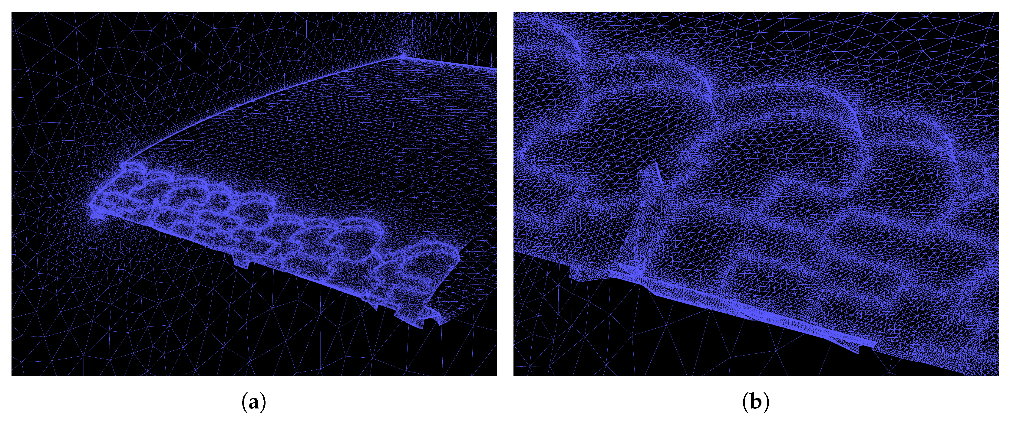
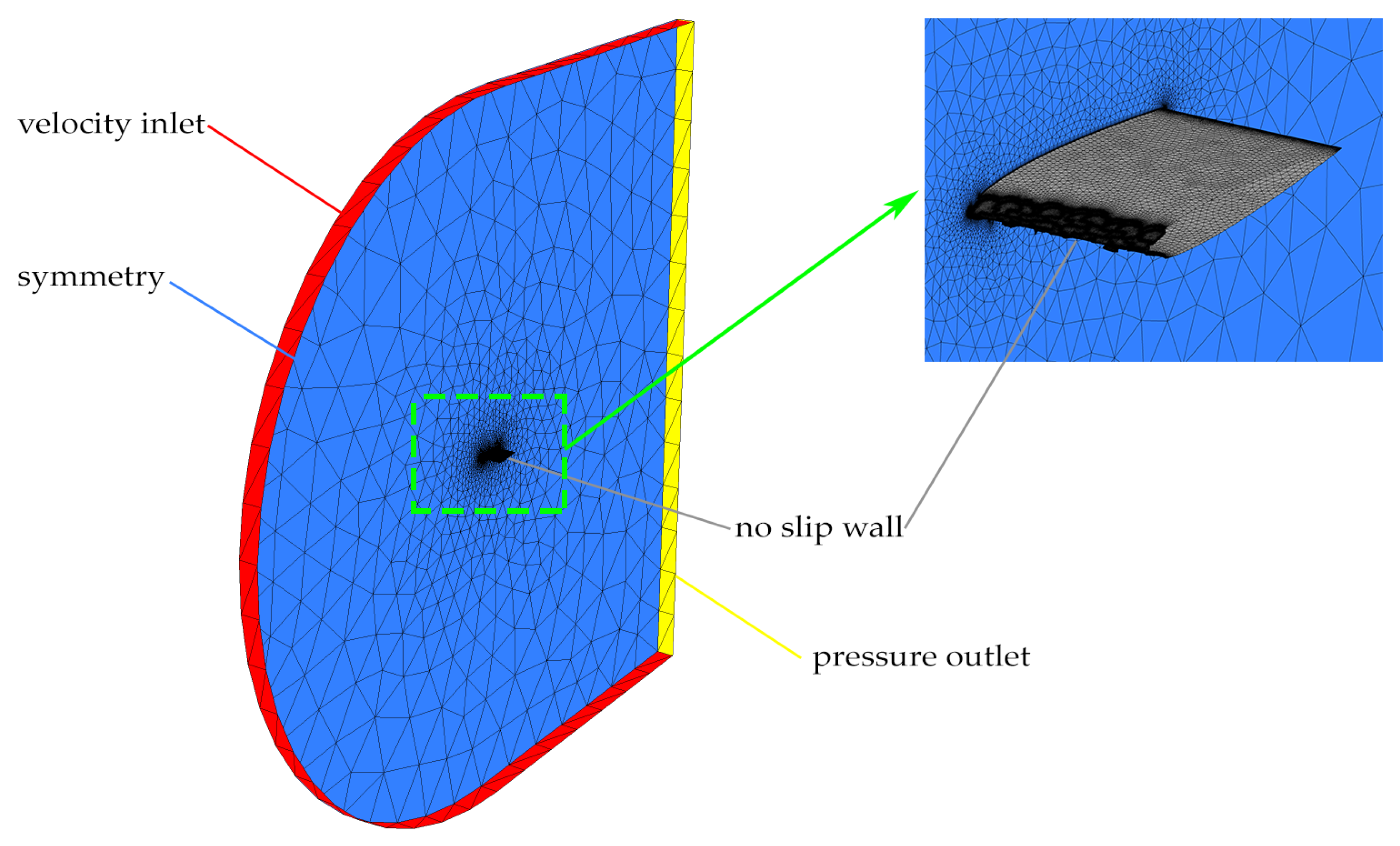
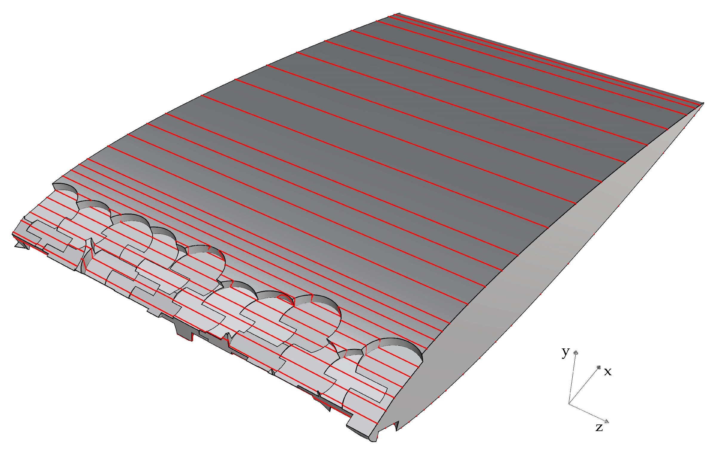
2.2. Three-Dimensional Setup

At first, we present the three-dimensional model. The latter is obtained by extruding the clean NACA 0012 airfoil and generating a damage pattern compatible with severe leading edge delamination. This stage of LEE is compatible with the damage observed in real blades after 10+ years of operating life [27,31]. Figure 2 reports the damaged blade model’s representation. With c being the chord length, this geometry has a span, b, of 0.65 c , an average delamination length of 0.1c, and a delamination depth of 0.014c. Since this model represents a blade element, no twist or tip effects have been considered. This approach is commonly used for this type of analysis (see, e.g., [34,51,52]). The model is simulated using a C-mesh with a radius of 12c and a wake region length of 12c in the streamwise direction. The fluid domain is obtained using Boolean subtraction between the C region and the blade.
A total of three hybrid increasingly refined grids are produced. These meshes are referred to as Coarse, Medium, and Fine with sizes of roughly 1.25, 2.50, and 5 million elements, respectively. The meshing process is carried out using the meshing software of the Ansys suite. Each grid quality is tested, resulting in a mean skewness of 0.34 and a mean orthogonal quality of 0.65. As previously stated, the meshing technique employs a hybrid structured–unstructured approach. An unstructured mesh is required to capture the blade’s complex three-dimensional features. Structured cells are used in the flow areas near the walls to improve resolution in the boundary layer and ensure that proper wall y-plus values, y w + = ρ w u τ y w / μ w , are kept. Here, ρ w and μ w denote the wall fluid density and viscosity, respectively, u τ = τ w / ρ w is the wall friction velocity, y w is the first-off-the-wall cell distance and τ w = μ w u p / y is the local wall friction, with u p being the local wall parallel speed. In particular, first guess of the first-off-the-wall cell distance, y w * , is obtained by enforcing a y-plus value of y w + = 0.5 to flat-plate empirical estimations according to the following equation:
y w * = 5.87 y w + μ ρ u R e 1 / 10
Here, u , ρ and μ denote the free stream velocity, flow density and viscosity, respectively, while R e is the Reynolds number of the flow. The near-wall resolution, in terms of y w + distribution, is verified a posteriori as reported in Section 3.2. Figure 3 reports a leading edge overview of the Fine grid, as well as an enlargement of the damaged zone.
The simulations are carried out using the Coupled scheme implemented in Ansys Fluent. The spatial discretization is treated with a 2nd-order upwind scheme, while the Least Squares Cell-Based (Ansys) approach is employed for gradients’ reconstruction. A precomputed tolerance of 1 × 10 6 is set as a stopping point for the iterative Navier–Stokes residuals dropping.
In terms of boundary conditions, the following are specified: velocity-inlet is enforced on the domain C edge while a pressure-outlet condition is set on the outlet section by selecting a reference value for the static pressure. The symmetry of the flow is enforced on the lateral boundaries. Figure 4 depicts an overview of the entire grid as well as boundary conditions. The inflow setup corresponds to a free stream Reynolds number of R e = ρ u c / μ = 3 × 10 5 .
Finally, initial conditions assume the flow at rest in the whole domain. From such a state, the Ansys Fluent hybrid initialization is used together with 10 iterations of the fmg-initialization procedure aiming to speed up the residuals convergence.

2.3. Two-Dimensional Setup

Concerning the two-dimensional model, Figure 5 reports the damaged airfoil’s geometrical properties. In particular, LEE is accounted for in a severely damaged NACA 0012. Thus, the 2D clean geometry is eroded accordingly, as seen in the sketch reported in Figure 5. With c being the chord of the airfoil, a delamination length of x = 0.1 c and a delamination depth of h = 0.014 c are considered, respectively. Such values fit the 3D arrangement at the average level. The model is simulated using a C-mesh with a radius of 12 c and a wake region length of 12 c in the streamwise direction. The fluid domain is obtained using Boolean subtraction between the C region and the airfoil, then it is divided into eight blocks with rectangular topology to produce a mapped grid.
Three mapped and increasingly refined meshes are used. The sizes are roughly 125 k, 250 k and 500 k for the Coarse, Medium and Fine grid, respectively. The meshing process is carried out using the mesh software of the Ansys suite. The quality of each grid is tested, resulting in a mean skewness of 0.34 and a mean orthogonal quality of 0.96. Each structured mesh is generated with a growth rate of 1.03 in the wall-normal direction to improve the boundary layer’s resolution and assure a proper wall y-plus distribution. The y w + < 1 threshold is pursued to provide a high-quality resolution of the near-wall flow. Similar procedures reported for the 3D setups are conducted to estimate the first guess of the first-off-the-wall cell distance. A posteriori verification of the y-plus distribution is reported in Section 3.1. Figure 6 reports an overview of the fine grid, as well as some enlargements of the leading edge and the delamination zone (Figure 6b,c).
Simulations are still carried out using the Coupled scheme implemented in Ansys Fluent, and the spatial discretization is still treated with a second-order upwind scheme. The same convergence tolerance, i.e., 1 × 10 6 , is used for monitoring the residual drop.
The boundary conditions are also kept equivalent to the 3D case. Thus, velocity-inlet is enforced on the domain C edge by specifying the inflowing speed such that R e = 3 × 10 5 . Pressure-outlet condition is set on the outlet section by specifying a reference value for the static pressure. Flow initializations follow the same procedure addressed for the 3D case.

3. Numerical Models Validation

This section aims at tuning and validating the two- and three-dimensional numerical models according the best CFD practice [53,54,55]. The analyses aim to determine the most appropriate mesh refinement level and establish the influence of the turbulence model on system behavior. For clarity, results related to the two-dimensional model are firstly presented.

3.1. Two-Dimensional CFD Model Validation

As initial step, we compare the global drag coefficient values of the clean airfoil at zero incidence as a function of the grid refinement and parametrically to the turbulence model. Thus, the drag coefficient per unit length, C d = D / q c , is compared to the experimental value C d E x p , the latter acquired in a in-house wind tunnel facility setting R e = 3 × 10 5 . Here, D is the drag force while q = 1 / 2 ρ u 2 is the free stream dynamic pressure. Results are reported in Figure 7a. According to the rescaling procedure, C d / C d E x p value close to 1 equals the experimental prediction. Due to the low-speed aerodynamics, the TSST model fits the best prediction. This result is consistent since the TSST model is tuned to describe the laminar-to-turbulent transition process, a key point for correctly predicting the wind turbine airfoils’ aerodynamic performance in low-Reynolds conditions [14,15]. Figure 7b also depicts the pressure coefficient, C p = ( p w p ) / q , trend obtained with the finest grid parametrically to the turbulence model. Since the airfoil is symmetrical and data are acquired at zero incidence ( α = 0 ) , the pressure distribution is symmetric, and a single curve is reported. Here, p w is the wall pressure while p denotes the free stream static pressure. The increasingly darker blue lines represent the data acquired with SA, k ω SST, and TSST model, respectively. The black dashed line denotes the XFOIL prediction [56], whereas the red triangles denote the experimentally acquired data by Gregory and O’Reilly [57]. Results are confined to a relatively tight range around experiments, except in a region near the trailing edge, where the TSST model overestimates the C p . In this concern, it should be recalled that pressure distribution by Gregory and O’Reilly [57] is acquired at a different Reynolds number. Simulations, in fact, are carried on at R e = 3 × 10 5 , while experiments refer to R e = 2.88 × 10 6 , leading to different behaviors in the boundary layer mechanics. Nevertheless, XFOIL viscous predictions at R e = 3.00 × 10 5 confirm the CFD pressure coefficient distribution. After these considerations, compliance with the experimental data assures that the pressure field is well captured by the CFD model, proving the quality of the numerical model via both global and local quantities.
As a further step in the validation process of the two-dimensional model, we trace the resolution of the near wall gradients. The clean geometry is still exploited as a reference for the grid tuning process. Thus, the wall y-plus value, y w + , and the local friction coefficient, C f = τ w / q , are investigated as a function of the turbulence model. Figure 8a reports the y w + distribution along the clean airfoil obtained with the finest grid. As the reader can observe, each of the three adopted models provides values around the recommended threshold for wall-resolved RANS simulations (i.e., y w + < 1 ), which allows us to state that, within the boundary layer, there is a sufficient number of points to resolve the velocity gradients near the walls accurately. The fine grid provides an average y w + value of 0.18 using the TSST model. This value is well below the recommended threshold for wall-turbulence estimation, allowing a large margin also for the simulation of the damaged geometry. In that case, in fact, different wall dynamics are expected, especially in the delamination zone, and y w + values closer to 1 are expected. Figure 8b reports the friction coefficient distribution. It can be observed that the SA and the k ω SST models’ predictions along the airfoil are very similar, while the TSST model provides for a recirculation zone on the final section of the airfoil. This fact is more consistent with the airfoil wall dynamics, making the TSST model outperform the other models concerning the experimental measurements. Such behavior is due to the low-Reynolds conditions of the flow. Thus, the ability of the TSST model to account for transition phenomena of the boundary layer is a fundamental aspect of predicting the flow physics correctly.
Finally, we conclude the two-dimensional model tuning by tracing its behavior in off-design conditions. Thus, the lift, C l , and drag, C d , coefficients distributions are obtained as a function of the angle of attack and compared with experimental data. Figure 9 reports the results of the analysis. Numerical data are still obtained with the most refined grid combined with the TSST model. High compatibility with experiments in a wide range of angles of attack is observed. In particular, the linear portion of the lift curve is very well captured by the steady-state RANS-TSST model (Figure 9a). While approaching stall conditions, RANS modeling struggles to capture the wake turbulent mechanics. This is why the CFD drag results do not perfectly fit the experimental data at high angles of attack (Figure 9b).
Based on these findings, the most refined grid combined with the TSST turbulence model is selected for the subsequent analyses. The model provides excellent agreement with the experimental data. In addition, offering an average y w + value of around 0.18, the model is promising to trace the flow physics even in off-design conditions.

3.2. Three-Dimensional CFD Model Validation

Following the two-dimensional model tuning, here we report the validation process concerning the three-dimensional arrangement. Since no experimental data are available to compare CFD outcomes, a mesh sensitivity study is carried out to establish the grid refinement level and the turbulence model in light of making results independent from the numerics. Thus, the global drag coefficient of the blade is gathered from three turbulence models (i.e., the SA, the k ω SST and the TSST models) and three increasingly refined meshes, fitting approximatively 1.25, 2.5, and 5 million elements, respectively. The drag coefficient values are scaled with the corresponding outcome obtained with the most refined setup combined with the TSST turbulence model, C d F i n e , T S S T . Such a rescaling choice is motivated by the fact that TSST model has shown the best results in the two-dimensional setup compared to the available experimental data.
Figure 10a summarize the outcome of the analysis. The reader can observe that very high compatibility is recovered among whole methodologies. The scaled C d values, in fact, are clustered to 1 as the mesh refinement level increases, regardless of how turbulence is accounted for. We observe that compared to the 2D case, in three-dimensional conditions, the TSST model does not outperform the others. The reason has to be found in the geometry damage, the latter triggering the separation of the boundary layer almost independently of the turbulence model, and even the SA one-equation model fits results independent of grid resolution. Thus, the fine mesh combined with the TSST is used to head the three-dimensional system mechanics.
Finally, we verify the mesh quality by tracing the y-plus wall values. Figure 10b provides the contour plot of the y w + . Again, the model confirms its quality since the near-wall resolution is consistently higher than the recommended thresholds for wall-resolved RANS simulations.

4. Results and Discussion

This section compares the 2D and the 3D damaged blades’ aerodynamic behaviour to highlight the differences and compatibilities between the two modeling approaches.

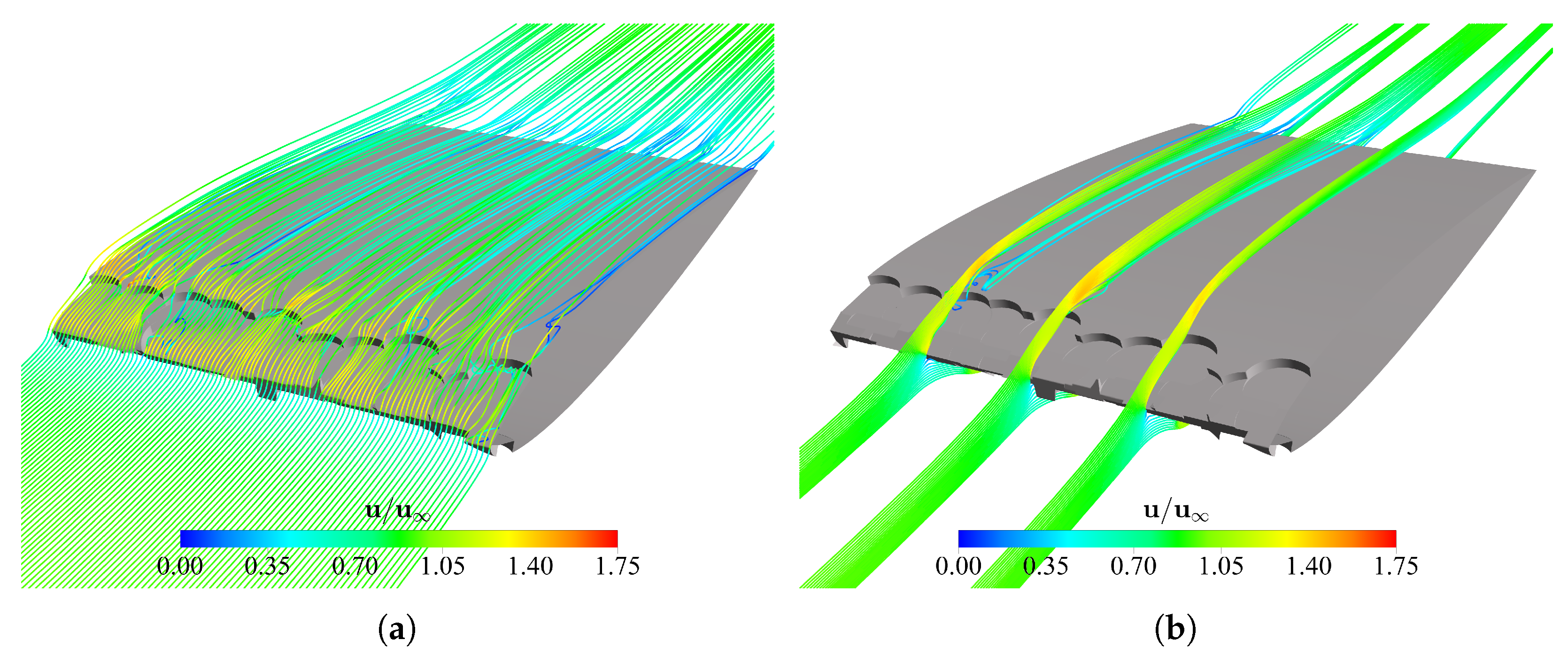
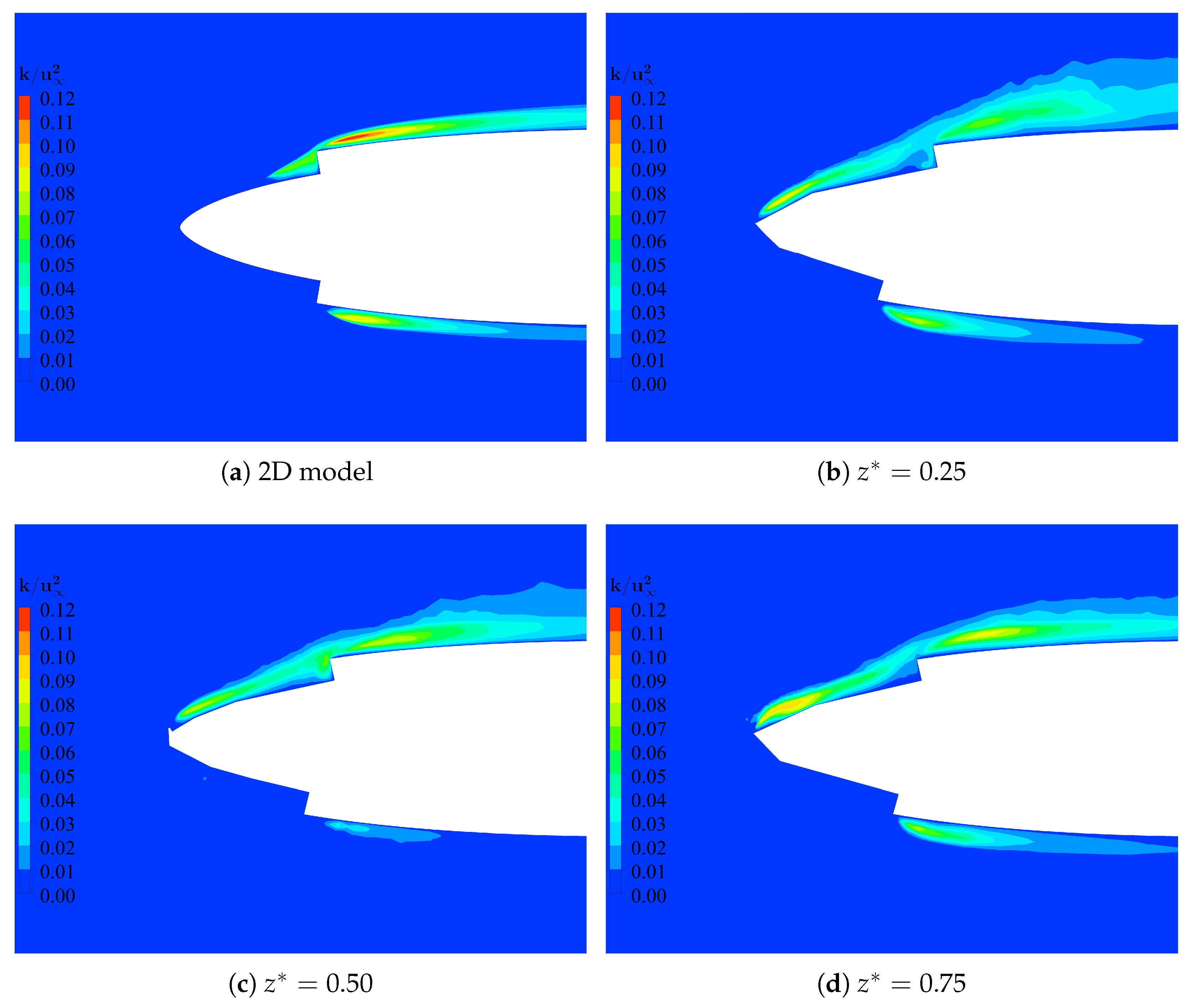
4.1. Flow Assessments Qualitative Comparison between 2D and 3D Models

Firstly, we remark on the flow configuration in a 3D path. Figure 11 shows the streamlines for the damaged blade with 4 incidence. The damaged blade’s flow mechanics is very complex since pathlines reveal several flow detachments and vortical structures, the latter induced by the erosion and the rough surface of the leading edge. In particular, geometrical features such as spikes and steps avoid flow streamlining, making the system’s macroscopic behavior strongly three-dimensional.
The friction coefficient distribution reveals further insights into the three-dimensional flow field. In particular, Figure 12 provides the comparison between the 0 and the 4 incidence configurations. Friction values abruptly increase on the various delaminated edges, the latter acting as an intense source of instability for the local boundary layer. The C f map suggests some clear patterns of the flow. In fact, vortices generated by the eroded leading edge are leaving a trace on the blade surface. The higher a vortex is, the tighter the friction coefficient trace becomes. Thus, since at α = 4 the boundary layer is substantially thicker than the zero incidence case, vortical structures are driven further from the surface, leading to narrower friction coherent traces.
Now a question arises. Can such a complex flow be modeled with a two-dimensional approach? Having a sufficiently accurate two-dimensional model is an undeniable advantage. The 3D setup, in fact, consists of about 5 million elements against the 500 k of the most resolved 2D model. Thus, working with a reliable 2D model would allow easily analyze any concern relating to the safe operation and expected life of a damaged wind turbines with an affordable computational cost. To answer this question first, we can look at the turbulent kinetic energy contours by comparing the 2D setup and several 3D damaged isosurfaces along the blade span. Figure 13 compares the contours of the dimensionless turbulent kinetic energy, k * = k / u 2 , as a function of the blade span for 2D and 3D models. The results refer to the 4 incidence configuration. Looking at the k * field, the two-dimensional model reasonably reproduces the three-dimensional assessment of the flow. Fluctuation patterns, in fact, look very similar regardless of the geometrical model on both the pressure and the suction sides, and the magnitude of the dimensionless turbulent kinetic energy are quantitatively comparable. The three-dimensional model exhibits slightly higher turbulent kinetic energy values immediately after the leading edge, and generally, the fluctuation zone is broader. This is due to the roughness effect induced by the leading edge’s sharp edges, which introduces more turbulence in the flow field. Conversely, having a rounded surface, the two-dimensional model produces lower turbulent energy. Thus, regardless of the strongly three-dimensionality of the flow field, the 2D and the 3D models show similar aerodynamics behaviors, at least at the velocity fluctuation level.
The following sections aim to trace the characteristics of the 2D damaged airfoil and compare its aerodynamics behavior with the clean reference geometry and the 3D arrangement. Pressure and friction coefficients, together with polar diagrams, will be examined.

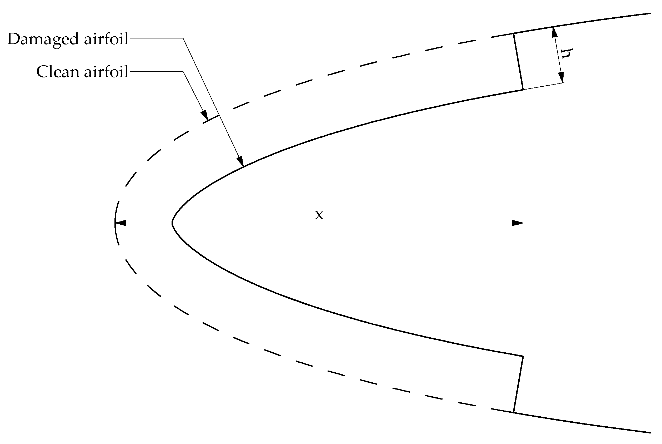
4.2. Clean and Damaged 2D Airfoil Comparison

As mentioned, to gradually increase the analysis complexity, we start by comparing the aerodynamics performance of the damaged 2D airfoil with the corresponding clean one. The same numerical model as presented in Section 3.1 is adopted for aerodynamic flow simulation of the damaged airfoil. Figure 14 compares the pressure coefficient trend distributions at various angles of attack. In particular, solid blue lines report variation of C p for the non-eroded airfoil behavior and red lines for the damaged airfoils. The reader can observe that the delamination zone causes a strong discontinuity in the pressure coefficient distribution, especially in low-incidence angles. This is due to the sudden deceleration of the airflow with consequent pressure recovery in this region, a fact that tends to mitigate its intensity as the incidence angle increases since the flow at the leading edge reduces its kinetic energy content. However, immediately after the eroded region, a strong suction is recorded. Far from the damaged zone, similar wall pressure values are recovered between the clean and the damaged configurations.
Figure 15 provides a comparison for the friction coefficient distributions. The same pattern is adopted, and, in particular, the damaged and the clean airfoil results are compared at different angles of attack. Only suction side distributions are shown to enhance the clarity of the results. Looking at the clean airfoil friction coefficient, the latter presents a steep rise in the damaged zone around the leading edge, followed by a smooth decrease until the C f = 0 condition is met. Flow detachment due to the low-Reynolds conditions happens near the trailing edge for the zero-angle of attack configuration and it moves toward the leading edge at higher incidence angles. The clean geometry smoothly regulates such a transition, and the separation location meets the leading edge at high incidence angles. Conversely, the leading edge erosion promotes an instantaneous recirculation of the boundary layer, and even for the zero-incidence case, the C f coefficient experiences negative values near the leading edge.
The difference of pressure and friction coefficients between the clean and the damaged case induces a significant reduction in the off-design eroded profile performance. In this regard, Figure 16 reports the polar diagrams comparison between the two geometries. The incidence values up to the stall condition are studied. To analyze the behavior of the airfoil beyond this condition, a non-stationary model should be set up, which is beyond the scope of this paper. Moreover, the most significant eroded areas are confined towards the blade tip, due to the higher rotational velocity. Airfoils in this area rarely experience very off-project angles of attack. Looking at Figure 15a, simulations predict the erosion to have a small impact on the lift coefficient at low incidences, while a more pronounced discrepancy is observed at higher angles of attack. Eroded airfoil drag polar plot, on the other hand, is systematically shifted upward by a value of 0.15–0.18 in the whole operation range. Thus, both C l and C d curves disclose a degradation of the aerodynamic performance of the damaged airfoil that generally increases with the angle of attack.

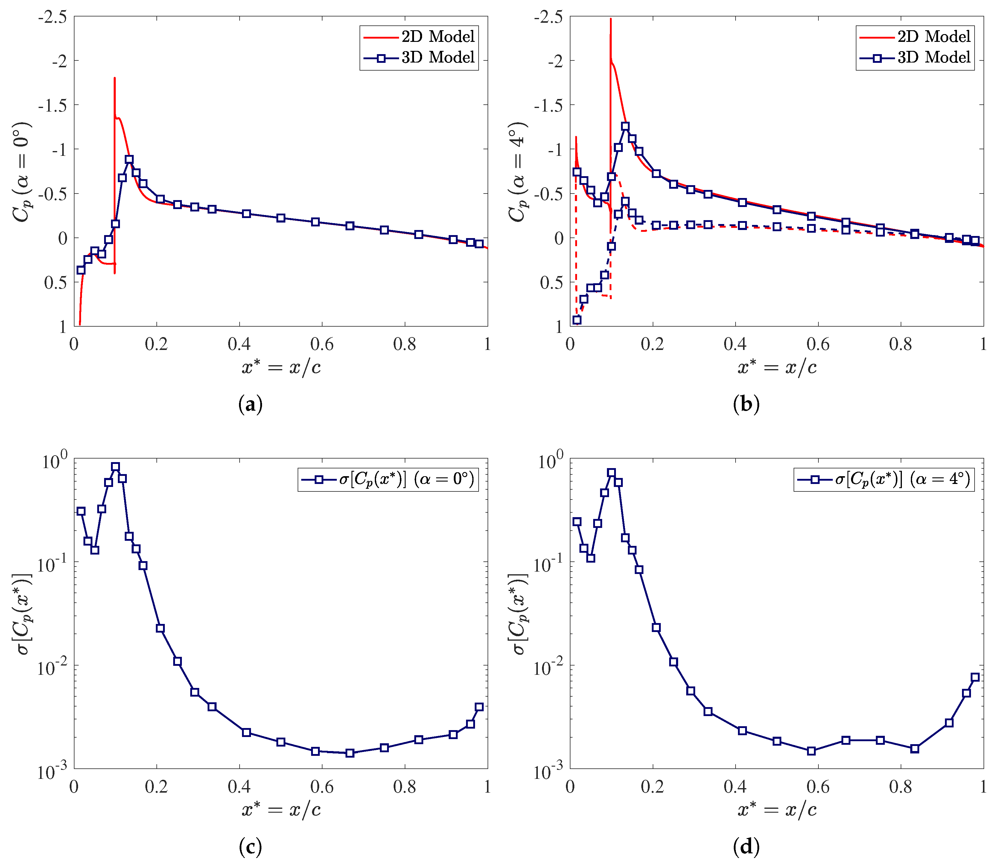
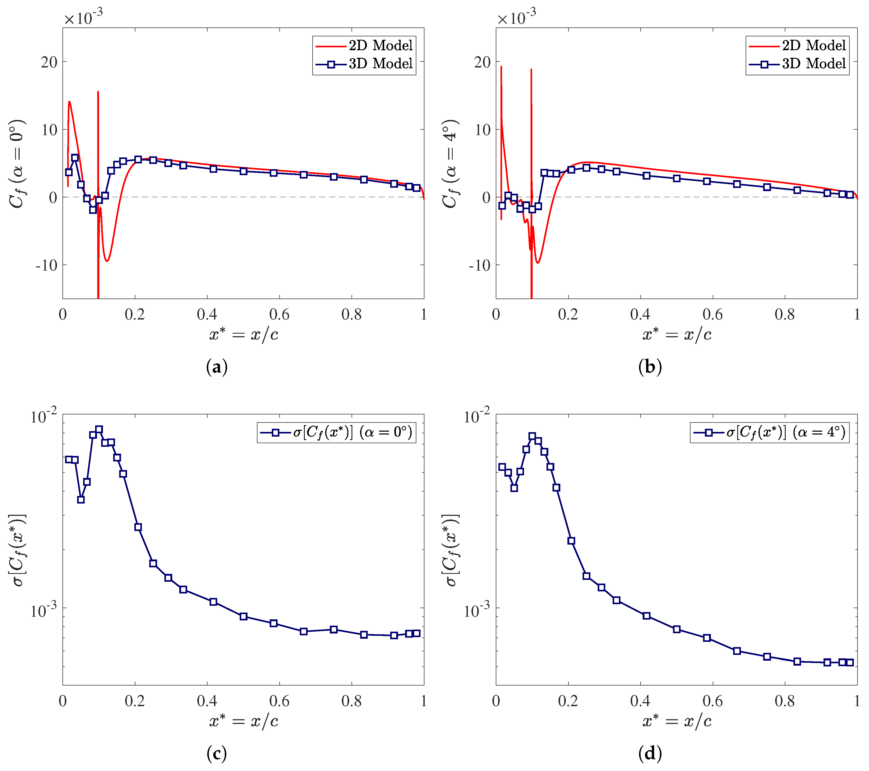
4.3. Damaged 3D Performance against 2D Eroded Assessment

Having understood the essential aspects relating to the damage 2D airfoil performance compared to the clean one, the present section aims to reach the aerodynamic characteristics of the 3D blade with the eroded 2D profile.
Since wall quantities depend on non-dimensional chordwise, x * = x / c and spanwise, z * = z / b , coordinates, wall properties are post-processed accordingly to spanwise-average operations. Thus, the three-dimensional spanwise-averaged coefficient distribution can be calculated from:
C x ¯ ( x i * ) = 1 N z k = 1 N z C x ( x i * , z k * )
Here, C x ( x i * , z k * ) denotes the N z pressure (or friction) coefficient values corresponding to a certain x i * and z k * blade surface location, the latter discretely selected as in Figure 17. Signal variations are then quantitatively traced by computing the root-mean-square of the difference between the local pressure and friction coefficient distributions and the respective spanwise-average values, as
σ C x x i * = 1 N z k = 1 N z C x x i * , z k * C x ¯ x i * 2
Results of the analysis are reported in Figure 18 and Figure 19. In particular, Figure 18 provides the three-dimensional spanwise-averaged pressure coefficient distribution, C p ¯ ( x * ) , compared to two-dimensional damaged reference. Results refer to the 0 (Figure 18a) and 4 (Figure 18b) incidence angles, respectively. As can be observed, although the flow is strongly three-dimensional, its mean characteristics are very closely fit by the two-dimensional eroded model. In particular, far from the area where the delaminated and healthy portion meet, the pressure field trend provided by the 2D model adheres perfectly to the forecast provided by the three-dimensional model. Mild discrepancies are detected around the geometrical jump. Here, in particular, the C p ¯ ( x * ) distribution shows a smoother behavior in the eroded region with a less marked discontinuity than the 2D airfoil values. This fact is easily explained since the two-dimensional setup is arranged so that a localized discontinuity perfectly uncouples the delaminate and the clean portions of the airfoil. Conversely, the three-dimensional model offers a complex pattern to deal with a realistic eroded leading edge. The latter induces an early separation of the flow in some areas with consequent coverage of part of the area of swirling flows and thickened boundary layer.
Figure 18c,d, on the other hand, provide the trend of σ [ C p ( x * ) ] along the blade. Here it is worth mentioning that such information can only be provided through a complete three-dimensional model. Nevertheless, the σ distribution makes it possible to verify a posteriori how significant the average data of the pressure coefficient is with respect to its true distribution. Thus, we observe that a maximum σ [ C p ( x * ) ] deviation of the order of unity is detected, the peak being clustered around x * = 0.1 where the geometrical discontinuity is nominally located. Conversely, far from the eroded area, the pressure coefficient fluctuations from the mean value are bounded in a small range, with an average of around 1 × 10 2 . Such a result allows us to state that the real three-dimensionality of the flow is clustered almost exclusively in the area where the eroded part is connected to the clean one, while elsewhere, the flow recovers its two-dimensional nature.
Having compared the pressure coefficient trends between the 2D and 3D models, we now move forward to the wall velocity gradients analysis by comparing the friction coefficient distributions and observing their average local fluctuations. Figure 19 reports the results of the analysis. Moreover, in this case it can be observed that the two-dimensional model well reproduces the friction coefficient’s global trend. In particular, far from erosion, the 2D and 3D predictions are almost superimposable both for the case with 0 (Figure 19a) and 4 (Figure 19b) angle of attacks. The most significant discrepancy between the two modeling methodologies is observed in the eroded area, where the 3D model always predicts a slightly anticipated flow separation, whereas the 2D model concentrates it almost exclusively around the geometric discontinuity.
The analysis of the root-mean-square deviation distributions (Figure 19c,d) shows that the 3D friction values are well confined around their average, with a deviation that does not exceed the second decimal digit. Nevertheless, if pressure coefficient distributions are impressively superimposed between the two-dimensional and three-dimensional model, a 3D eroded pattern leads to more significant discrepancies in the boundary layer flow mechanics, with consequent less compatibility between the 2D and 3D friction coefficients.
Finally, Figure 20 compares the off-design behavior of the 2D and 3D arrangements by displaying the lift and drag coefficient distributions as a function of the angle of attack. As expected, the lift coefficient trends for the 2D and 3D configurations are almost identical (Figure 20a). This is because the 2D and 3D pressure fields are effectively equivalent at an extensive range of angles of attack, resulting in a similar lift coefficient between the two modeling techniques. On the other hand, the three-dimensional model’s drag coefficient is systematically higher (by roughly 17%) than in the damaged 2D instance (Figure 20b). This is owing to the differing wall dynamics experienced by the 3D geometry near the leading edge. Although the friction coefficient is an essential factor in predicting blade aerodynamics, in any digital twin model that aims at evaluating a wind turbine’s service life would have the primary goal of accurately estimating the lift coefficient. Such a parameter, in fact, is the primary contributor to yearly electricity production, and as such, it is the critical datum for estimating maintenance interventions. As a result of present investigations, a simple eroded 2D model, adequately calibrated, has been shown to thoroughly represent the overall aerodynamics of a wind turbine blade under eroded leading edge conditions at a much lower computational cost than a fully 3D setup. In particular, present analyses are performed on a workstation composed of 2 Intel ® Xeon ® X5650 CPUs and 24GB of RAM. With such an architecture, two-dimensional simulations took about 30 min to get the convergence of the flow quantities, while 3D cases take about 15 h. Thus, the computational cost of the 2D model is negligible compared to the 3D approach, making 2D modeling an underlying basis in defining a digital twin for predicting the service life of a wind turbine.

5. Conclusions

The present work compares three-dimensional CFD RANS modeling of leading-edge eroded wind turbine blades with simplified two-dimensional setups.
First, the numerical models’ behavior is evaluated to establish the optimal arrangement for grid resolution and turbulence model. Thus, a validation campaign with experimental data is reported for global and local quantity convergence, determining the optimal mesh refinement level and the most appropriate turbulence model for predicting the airfoil and the blade aerodynamic performance at low Reynolds numbers which are experienced in wind turbines operation. According to our analyses, a 500 k-element 2D assessment coupled with the TSST model provides a good balance between computational time and accuracy, while a 5 million-element 3D setup, always combined with the TSST model, ensures grid independency for the blade aerodynamics.
Qualitative (i.e., observation of fluid fields) and quantitative observations (i.e., analysis of wall flow properties) are then provided. From the first set of analyses, we found that, regardless of the strongly three-dimensionality behavior of the blade, 2D and 3D turbulent kinetic energy fields are closely similar. This encourages us to address deeper comparison levels by looking at pressure and friction coefficient distribution as well as the polar diagrams. Quantitative observations show that the 2D approach accurately fits surface pressure trends, as well as excellent agreements in lift coefficient in a wide range of angles of attack are recovered. On the other hand, a systematic underestimation of the drag coefficient of about 17% in the whole range of operations is observed. The outcomes of this research are crucial since they confirm that the system’s inviscid characteristics (i.e., pressure distribution and lift coefficient) are not characterized by extremely three-dimensional effects and that a simplified two-dimensional model can forecast their trends accurately. Thus, a reduced-order model can well represent the more significant characteristics of the complex three-dimensional severely eroded blade, and do so at a much lower computational cost. In addition, since the lift coefficient is the fundamental parameter for forecasting the AEP of a wind power plant, simplified 2D models like the one proposed by the authors may serve as a foundation for simplified predictive models of the wind farm’s working life accounting for blade erosion.
Future works will investigate other stages of the erosion process as well propose an algebraic model calibrated on CFD data to determine the operating life of wind turbines accounting for the erosion of the leading edge.

Author Contributions

Conceptualization, F.D.V.; methodology, M.C. and F.D.V.; software, M.C. and F.D.V.; validation, M.C., F.D.V.; formal analysis, M.C. and F.D.V.; investigation, M.C. and F.D.V.; resources, M.C., F.D.V., E.B., F.Z. and H.H.; data curation, M.C. and F.D.V.; writing—original draft preparation, F.D.V.; writing—review and editing, M.C., F.D.V., E.B., F.Z., A.H. and H.H.; visualization, M.C., F.D.V., E.B. and H.H.; supervision, F.D.V. and E.B.; project administration, F.D.V. All authors have read and agreed to the published version of the manuscript.

Funding

This research received no external funding.

Institutional Review Board Statement

Not applicable.

Informed Consent Statement

Not applicable.

Data Availability Statement

Not applicable.

Conflicts of Interest

The authors declare no conflict of interest.

Abbreviations

The following abbreviations are used in this manuscript:
AEPAnnual Energy Production
CFDComputational Fluid Dynamics
LEELeading Edge Erosion
PSPressure Side
RANSReynolds-Averaged Navier–Stokes
SASpalart–Allmaras
SSSuction Side
SSTShear Stress Transport
TSSTTransition Shear Stress Transport

References

  1. Wind Europe. Wind Energy in Europe: 2021 Statistics and the Outlook for 2022–2026; Technical Report; Wind Europe: Brussels, Belgium, 2022; Available online: https://windeurope.org/intelligence-platform/product/wind-energy-in-europe-2021-statistics-and-the-outlook-for-2022-2026/ (accessed on 11 August 2022).
  2. IRENA. Renewable Energy Statistics 2022; Technical Report; The International Renewable Energy Agency: Abu Dhabi, UAE, 2022; Available online: https://irena.org/publications/2022/Apr/Renewable-Capacity-Statistics-2022 (accessed on 11 August 2022).
  3. Butterfield, C.P.; Scott, G.; Musial, W. Comparison of wind tunnel airfoil performance data with wind turbine blade data. J. Sol. Energy Eng. 1992, 114, 119–124. [Google Scholar] [CrossRef]
  4. Somers, D.M.; Tangler, J.L. Wind tunnel test of the S814 thick root airfoil. J. Sol. Energy Eng. 1996, 118, 217–221. [Google Scholar] [CrossRef]
  5. Devinant, P.; Laverne, T.; Hureau, J. Experimental study of wind-turbine airfoil aerodynamics in high turbulence. J. Wind Eng. Ind. Aerodyn. 2002, 90, 689–707. [Google Scholar] [CrossRef]
  6. Selig, M.S.; McGranahan, B.D. Wind tunnel aerodynamic tests of six airfoils for use on small wind turbines. J. Sol. Energy Eng. 2004, 126, 986–1001. [Google Scholar] [CrossRef]
  7. Chamorro, L.P.; Porté-Agel, F. A wind-tunnel investigation of wind-turbine wakes: Boundary-layer turbulence effects. Bound.-Layer Meteorol. 2009, 132, 129–149. [Google Scholar] [CrossRef]
  8. Chamorro, L.P.; Porté-Agel, F. Effects of thermal stability and incoming boundary-layer flow characteristics on wind-turbine wakes: A wind-tunnel study. Bound.-Layer Meteorol. 2010, 136, 515–533. [Google Scholar] [CrossRef]
  9. Chamorro, L.P.; Porte-Agel, F. Turbulent flow inside and above a wind farm: A wind-tunnel study. Energies 2011, 4, 1916–1936. [Google Scholar] [CrossRef]
  10. Adaramola, M.; Krogstad, P.Å. Experimental investigation of wake effects on wind turbine performance. Renew. Energy 2011, 36, 2078–2086. [Google Scholar] [CrossRef]
  11. Sun, H.; Gao, X.; Yang, H. A review of full-scale wind-field measurements of the wind-turbine wake effect and a measurement of the wake-interaction effect. Renew. Sustain. Energy Rev. 2020, 132, 110042. [Google Scholar] [CrossRef]
  12. Porté-Agel, F.; Bastankhah, M.; Shamsoddin, S. Wind-turbine and wind-farm flows: A review. Bound.-Layer Meteorol. 2020, 174, 1–59. [Google Scholar] [CrossRef] [Green Version]
  13. Yang, S.; Chang, Y.; Arici, O. Incompressible Navier-Stokes computation of the NREL airfoils using a symmetric total variational diminishing scheme. J. Solar Energy Eng. 1994, 116, 174–182. [Google Scholar] [CrossRef]
  14. Wolfe, W.; Ochs, S.; Wolfe, W.; Ochs, S. CFD calculations of S809 aerodynamic characteristics. In Proceedings of the 35th Aerospace Sciences Meeting and Exhibit, Reno, NV, USA, 6–9 January 1997; p. 973. [Google Scholar] [CrossRef]
  15. Munduate, X.; Ferrer, E. CFD predictions of transition and distributed roughness over a wind turbine airfoil. In Proceedings of the 47th AIAA Aerospace Sciences Meeting Including the New Horizons Forum and Aerospace Exposition, Orlando, FL, USA, 5–8 January 2009; p. 269. [Google Scholar] [CrossRef]
  16. Sanderse, B.; Van der Pijl, S.; Koren, B. Review of computational fluid dynamics for wind turbine wake aerodynamics. Wind Energy 2011, 14, 799–819. [Google Scholar] [CrossRef]
  17. Mittal, A.; Sreenivas, K.; Taylor, L.K.; Hereth, L.; Hilbert, C.B. Blade-resolved simulations of a model wind turbine: Effect of temporal convergence. Wind Energy 2016, 19, 1761–1783. [Google Scholar] [CrossRef]
  18. Van der Laan, M.; Hansen, K.S.; Sørensen, N.N.; Réthoré, P.E. Predicting Wind Farm Wake Interaction with RANS: An Investigation of the Coriolis Force; Journal of Physics: Conference Series; IOP Publishing: Bristol, UK, 2015; Volume 625, p. 012026. [Google Scholar] [CrossRef]
  19. Astolfi, D.; Castellani, F.; Terzi, L. A study of wind turbine wakes in complex terrain through RANS simulation and SCADA data. J. Solar Energy Eng. 2018, 140. [Google Scholar] [CrossRef]
  20. Zhong, W.; Tang, H.; Wang, T.; Zhu, C. Accurate RANS simulation of wind turbine stall by turbulence coefficient calibration. Appl. Sci. 2018, 8, 1444. [Google Scholar] [CrossRef]
  21. Mehta, D.; Van Zuijlen, A.; Koren, B.; Holierhoek, J.; Bijl, H. Large Eddy Simulation of wind farm aerodynamics: A review. J. Wind Eng. Ind. Aerodyn. 2014, 133, 1–17. [Google Scholar] [CrossRef]
  22. Thé, J.; Yu, H. A critical review on the simulations of wind turbine aerodynamics focusing on hybrid RANS-LES methods. Energy 2017, 138, 257–289. [Google Scholar] [CrossRef]
  23. Stevens, R.J.; Martínez-Tossas, L.A.; Meneveau, C. Comparison of wind farm large eddy simulations using actuator disk and actuator line models with wind tunnel experiments. Renew. Energy 2018, 116, 470–478. [Google Scholar] [CrossRef]
  24. Solís-Gallego, I.; Argüelles Díaz, K.M.; Fernández Oro, J.M.; Velarde-Suárez, S. Wall-resolved LES modeling of a wind turbine airfoil at different angles of attack. J. Marine Sci. Eng. 2020, 8, 212. [Google Scholar] [CrossRef]
  25. Vermeer, L.; Sørensen, J.N.; Crespo, A. Wind turbine wake aerodynamics. Prog. Aerosp. Sci. 2003, 39, 467–510. [Google Scholar] [CrossRef]
  26. Enevoldsen, P.; Xydis, G. Examining the trends of 35 years growth of key wind turbine components. Energy Sustain. Dev. 2019, 50, 18–26. [Google Scholar] [CrossRef]
  27. Keegan, M.H.; Nash, D.; Stack, M. On erosion issues associated with the leading edge of wind turbine blades. J. Phys. D: Appl. Phys. 2013, 46, 383001. [Google Scholar] [CrossRef]
  28. Rempel, L. Rotor blade leading edge erosion-real life experiences. Wind Syst. Mag. 2012, 11, 22–24. Available online: http://windaction.s3.amazonaws.com/attachments/2310/1012_BladeFeature.pdf (accessed on 11 August 2022).
  29. Dalili, N.; Edrisy, A.; Carriveau, R. A review of surface engineering issues critical to wind turbine performance. Renew. Sustain. Energy Rev. 2009, 13, 428–438. [Google Scholar] [CrossRef]
  30. Ehrmann, R.S.; White, E.B.; Maniaci, D.C.; Chow, R.; Langel, C.M.; Van Dam, C.P. Realistic leading-edge roughness effects on airfoil performance. In Proceedings of the 31st AIAA Applied Aerodynamics Conference, San Diego, CA, USA, 24 June 2013; p. 2800. [Google Scholar] [CrossRef]
  31. Sareen, A.; Sapre, C.A.; Selig, M.S. Effects of leading edge erosion on wind turbine blade performance. Wind Energy 2014, 17, 1531–1542. [Google Scholar] [CrossRef]
  32. Gaudern, N. A Practical Study of the Aerodynamic Impact of Wind Turbine Blade Leading Edge Erosion; Journal of Physics: Conference Series; IOP Publishing: Bristol, UK, 2014; Volume 524, p. 012031. [Google Scholar] [CrossRef]
  33. Langel, C.M.; Chow, R.; Hurley, O.F.; Van Dam, C.C.P.; Maniaci, D.C.; Ehrmann, R.S.; White, E.B. Analysis of the impact of leading edge surface degradation on wind turbine performance. In Proceedings of the 33rd Wind Energy Symposium, Kissimmee, FL, USA, 5–9 January 2015; p. 0489. [Google Scholar] [CrossRef]
  34. Maniaci, D.C.; White, E.B.; Wilcox, B.; Langel, C.M.; van Dam, C.; Paquette, J.A. Experimental Measurement and CFD Model Development of Thick Wind Turbine Airfoils with Leading Edge Erosion; Journal of Physics: Conference Series; IOP Publishing: Bristol, UK, 2016; Volume 753, p. 022013. [Google Scholar] [CrossRef]
  35. Han, W.; Kim, J.; Kim, B. Effects of contamination and erosion at the leading edge of blade tip airfoils on the annual energy production of wind turbines. Renew. Energy 2018, 115, 817–823. [Google Scholar] [CrossRef]
  36. Elhadi Ibrahim, M.; Medraj, M. Water droplet erosion of wind turbine blades: Mechanics, testing, modeling and future perspectives. Materials 2019, 13, 157. [Google Scholar] [CrossRef]
  37. Dashtkar, A.; Hadavinia, H.; Sahinkaya, M.N.; Williams, N.A.; Vahid, S.; Ismail, F.; Turner, M. Rain erosion-resistant coatings for wind turbine blades: A review. Polym. Polym. Compos. 2019, 27, 443–475. [Google Scholar] [CrossRef]
  38. Shankar Verma, A.; Jiang, Z.; Ren, Z.; Hu, W.; Teuwen, J.J. Effects of onshore and offshore environmental parameters on the leading edge erosion of wind turbine blades: A comparative study. J. Offshore Mech. Arct. Eng. 2021, 143. [Google Scholar] [CrossRef]
  39. Law, H.; Koutsos, V. Leading edge erosion of wind turbines: Effect of solid airborne particles and rain on operational wind farms. Wind Energy 2020, 23, 1955–1965. [Google Scholar] [CrossRef]
  40. Castorrini, A.; Cappugi, L.; Bonfiglioli, A.; Campobasso, M. Assessing Wind Turbine Energy Losses due to Blade Leading Edge Erosion Cavities with Parametric CAD and 3D CFD; Journal of Physics: Conference Series; IOP Publishing: Bristol, UK, 2020; Volume 1618, p. 052015. [Google Scholar] [CrossRef]
  41. Wang, Y.; Wang, L.; Duan, C.; Zheng, J.; Liu, Z.; Ma, G. CFD simulation on wind turbine blades with leading edge erosion. J. Theor. Appl. Mech. 2021, 59. [Google Scholar] [CrossRef]
  42. Ortolani, A.; Castorrini, A.; Campobasso, M.S. Multi-Scale Navier-Stokes Analysis of Geometrically Resolved Erosion of Wind Turbine Blade Leading Edges; Journal of Physics: Conference Series; IOP Publishing: Bristol, UK, 2022; Volume 2265, p. 032102. [Google Scholar] [CrossRef]
  43. Mishnaevsky, L., Jr.; Hasager, C.B.; Bak, C.; Tilg, A.M.; Bech, J.I.; Rad, S.D.; Fæster, S. Leading edge erosion of wind turbine blades: Understanding, prevention and protection. Renew. Energy 2021, 169, 953–969. [Google Scholar] [CrossRef]
  44. Eisenberg, D.; Laustsen, S.; Stege, J. Wind turbine blade coating leading edge rain erosion model: Development and validation. Wind Energy 2018, 21, 942–951. [Google Scholar] [CrossRef]
  45. ANSYS. ANSYS 19.2 FLUENT User’s Guide; ANSYS: Canonsburg, PA, USA, 2018. [Google Scholar]
  46. MATLAB. 9.7. 0.1190202 (R2019b); MathWorks Inc.: Natick, MA, USA, 2018; Available online: https://it.mathworks.com/products/new_products/release2019b.html (accessed on 11 August 2022).
  47. Spalart, P.; Allmaras, S. A one-equation turbulence model for aerodynamic flows. In Proceedings of the 30th Aerospace Sciences Meeting and Exhibit, Reno, NV, USA, 6–9 January 1992; p. 439. [Google Scholar] [CrossRef]
  48. Menter, F.R. Two-equation eddy-viscosity turbulence models for engineering applications. AIAA J. 1994, 32, 1598–1605. [Google Scholar] [CrossRef]
  49. Menter, F.R.; Langtry, R.B.; Likki, S.; Suzen, Y.; Huang, P.; Völker, S. A correlation-based transition model using local variables—Part I: Model formulation. J. Turbomach. 2006, 128, 413–422. [Google Scholar] [CrossRef]
  50. ANSYS FLUENT Theory Guide. Available online: https://www.afs.enea.it/project/neptunius/docs/fluent/html/th/main_pre.htm (accessed on 11 August 2022).
  51. Campobasso, M.S.; Castorrini, A.; Cappugi, L.; Bonfiglioli, A. Experimentally validated three-dimensional computational aerodynamics of wind turbine blade sections featuring leading edge erosion cavities. Wind Energy 2022, 25, 168–189. [Google Scholar] [CrossRef]
  52. Sapre, C. Turbine Blade Erosion and the Use of Wind Protection Tape. 2012. Available online: https://www.ideals.illinois.edu/items/31357 (accessed on 11 August 2022).
  53. Avanzi, F.; De Vanna, F.; Ruan, Y.; Benini, E. Design-Assisted of Pitching Aerofoils through Enhanced Identification of Coherent Flow Structures. Designs 2021, 5, 11. [Google Scholar] [CrossRef]
  54. De Vanna, F.; Bof, D.; Benini, E. Multi-Objective RANS Aerodynamic Optimization of a Hypersonic Intake Ramp at Mach 5. Energies 2022, 15, 2811. [Google Scholar] [CrossRef]
  55. De Vanna, F.; Picano, F.; Benini, E.; Quinn, M.K. Large-Eddy Simulations of the Unsteady Behavior of a Hypersonic Intake at Mach 5. AIAA J. 2021, 59, 3859–3872. [Google Scholar] [CrossRef]
  56. Drela, M. XFOIL: An analysis and design system for low Reynolds number airfoils. In Low Reynolds Number Aerodynamics; Springer: Berlin, Germany, 1989; pp. 1–12. [Google Scholar] [CrossRef]
  57. Gregory, N.; O’Reilly, C. Low-Speed Aerodynamic Characteristics of NACA 0012 Aerofoil Section, Including the Effects of Upper-Surface Roughness Simulating Hoar Frost. ARC, R&M-3726. 1970. Available online: https://reports.aerade.cranfield.ac.uk/handle/1826.2/3003 (accessed on 11 August 2022).
Figure 1. Various levels of erosion from lighter (left) to heavier (right), adapted from [44].
Fluids 07 00302 g001
Figure 2. Geometrical representation of the three-dimensional blade with LEE.
Fluids 07 00302 g002
Figure 3. Mesh overview (a) and detail (b) of the three-dimensional geometry. The figures refer to the fine grid of 5 million elements.
Fluids 07 00302 g003
Figure 4. Boundary conditions overview: the red surface is the velocity-inlet while the pressure-outlet is highlighted in yellow. To enhance clarity only one side boundary, with symmetry condition imposed, is shown in light blue.
Fluids 07 00302 g004
Figure 5. Geometrical representation of the LEE configuration. The chordwise delamination extent is denoted with the letter x and the delamination depth is denoted with the letter h.
Fluids 07 00302 g005
Figure 6. Mesh overview (a) and details (b,c). The figures refer to the fine grid of 500 k elements.
Fluids 07 00302 g006
Figure 7. Two-dimensional model validation. (a) Comparison between the experimental and the CFD-computed drag coefficient of the undamaged NACA 0012 airfoil as a function of the turbulence model and the mesh refinement level; (b) Pressure coefficient distribution as a function of the turbulence model obtained using the finest grid. Red triangles denote the pressure coefficient experimentally acquired by Gregory and O’Reilly [57]. Single curve reported being the flow symmetric.
Fluids 07 00302 g007
Figure 8. Wall y + and friction coefficient trends as a function of the turbulence model obtained with the finest grid. (a) y w + distribution on the airfoil surface; (b) C f distribution on the airfoil surface.
Fluids 07 00302 g008
Figure 9. Comparison between lift and drag polar diagrams obtained with the finest grid (using the TSST turbulence model) and the experimental data for NACA 0012 airfoil. (a) C l as a function of the incidence; (b) C d as a function of the incidence.
Fluids 07 00302 g009
Figure 10. Three-dimensional model validation. (a) CFD-computed drag coefficient of the damaged blade as a function of the turbulence model and the mesh refinement level; (b) Wall y + contour obtained with the finest grid and the TSST model at 0 incidence.
Fluids 07 00302 g010
Figure 11. Streamlines around the damaged blade at 4 incidence. (a) Streamlines on the suction side of the blade; (b) Streamlines in three x y planes passing through 1 / 4 , 1 / 2 , and 3 / 4 of the span.
Fluids 07 00302 g011
Figure 12. Comparison between contour plots of the friction coefficient on the damaged blade at 0 incidence and 4 incidence. (a) C f contour at α = 0 ; (b) C f contour at α = 4 .
Fluids 07 00302 g012
Figure 13. Comparison between contour plots of the non-dimensional turbulent kinetic energy around the 2D airfoil (a) and the 3D blade (bd) at 4 incidence. (a) Turbulent kinetic energy contour around the two-dimensional airfoil; (bd) turbulent kinetic energy contour around the three-dimensional blade on a x y plane passing through 1 / 4 , 1 / 2 , and 3 / 4 of the span, respectively.
Fluids 07 00302 g013
Figure 14. Pressure coefficients comparison between the clean airfoil and the damaged airfoil: the distribution on the Pressure Side (PS) is denoted with the dashed line, while the continuous line is used for the Suction Side (SS) trends. (a) C p distribution at 0 incidence; (b) C p distribution at 4 incidence; (c) C p distribution at 8 incidence; (d) C p distribution at 12 incidence.
Fluids 07 00302 g014
Figure 15. Friction coefficients comparison between the clean airfoil and the damaged airfoil. C f distribution at (a) 0 incidence; (b) 4 incidence; (c) 8 incidence; (d) 12 incidence.
Fluids 07 00302 g015
Figure 16. Comparison between polar diagrams of the clean airfoil and the damaged airfoil. (a) C l polar plot comparison; (b) C d polar plot comparison.
Fluids 07 00302 g016
Figure 17. Geometrical representation of the lines where friction and pressure coefficient are evaluated.
Fluids 07 00302 g017
Figure 18. Pressure coefficients comparison between the 2D damaged airfoil and the 3D eroded blade. Distributions on the pressure side are denoted with the dashed line while solid lines are used for suction side trends. Dark blue squares denote the C p ¯ ( x * ) value over the three-dimensional blade. (a) Pressure coefficients comparison at 0 incidence; (b) Pressure coefficients comparison at 4 incidence; (c) Pressure coefficient standard deviation on the blade at 0 incidence; (d) Pressure coefficient standard deviation on the blade at 4 incidence.
Fluids 07 00302 g018
Figure 19. Friction coefficients comparison between the 2D damaged airfoil and the 3D eroded blade. Dark blue squares denote the C f ¯ ( x * ) value over the three-dimensional blade. (a) C f distribution at 0 incidence; (b) C f distribution at 4 incidence; (c) Friction coefficient standard deviation on the blade at 0 incidence; (d) Friction coefficient standard deviation on the blade at 4 incidence.
Fluids 07 00302 g019
Figure 20. Comparison between polar diagrams of the 2D damaged airfoil and the 3D eroded blade. (a) Comparison of the lift coefficient distribution as a function of the angle of attack; (b) Comparison of the drag coefficient distribution as a function of the angle of attack.
Fluids 07 00302 g020
Publisher’s Note: MDPI stays neutral with regard to jurisdictional claims in published maps and institutional affiliations.

