
Evaluation of Turbulence Models in Unsteady Separation


Department of Mechanical and Materials Engineering, Queen’s University, Kingston, ON K7L3N6, Canada
*
Author to whom correspondence should be addressed.
†
Current address: Department of Mechanical Engineering, Stanford University, Stanford, CA 94305, USA.
Fluids 2023, 8(10), 273; https://doi.org/10.3390/fluids8100273
Submission received: 23 August 2023
/
Revised: 24 September 2023
/
Accepted: 28 September 2023
/
Published: 7 October 2023
(This article belongs to the Special Issue Next-Generation Methods for Turbulent Flows)
Abstract
:Unsteady separation is a phenomenon that occurs in many flows and results in increased drag, decreased lift, noise emission, and loss of efficiency or failure in flow devices. Turbulence models for the steady or unsteady Reynolds-averaged Navier–Stokes equations (RANS and URANS, respectively) are commonly used in industry; however, their performance is often unsatisfactory. The comparison of RANS results with experimental data does not clearly isolate the modeling errors, since differences with the data may be due to a combination of modeling and numerical errors, and also to possible differences in the boundary conditions. In the present study, we use high-fidelity large-eddy simulation (LES) results to carry out a consistent evaluation of the turbulence models. By using the same numerical scheme and boundary conditions as the LES, and a grid on which grid convergence was achieved, we can isolate modeling errors. The calculations (both LES and RANS) are carried out using a well-validated, second-order-accurate code. Separation is generated by imposing a freestream velocity distribution, that is modulated in time. We examined three frequencies (a rapid, flutter-like oscillation, an intermediate one in which the forcing and the flow have the same timescales, and a quasi-steady one). We also considered three different pressure distributions, one with alternating favorable and adverse pressure gradients (FPGs and APGs, respectively), one oscillating between an APG and a zero-pressure gradient (ZPG), and one with an oscillating APG. All turbulence models capture the general features of this complex unsteady flow as well or better than in similar steady cases. The presence, during the cycle, of times in which the freestream pressure-gradient is close to zero affects significantly the model performance. Comparing our results with those in the literature indicates that numerical errors due to the type of discretization and the grid resolution are as significant as those due to the turbulence model.
1. Introduction
1.1. Motivation
Separation is a phenomenon that occurs frequently in engineering and the natural sciences. It significantly affects the flow dynamics, such as the forces on immersed objects or the effective area (and the pressure distribution) in diverging ducts. Separation typically causes a decrease in the efficiency of devices such as turbomachines, diffusers and lifting bodies due to increased drag and decreased lift. The phenomenon may induce noise, unwanted vibrations, and significant stress on turbomachinery [1]. Because of its ubiquity, separation has been the subject of a considerable amount of work [1,2,3,4,5,6,7]. Separation can be caused by sharp geometrical changes or by strong APGs. This work focuses on pressure-induced separation, in which boundary layer detachment happens solely due to a strong APG.
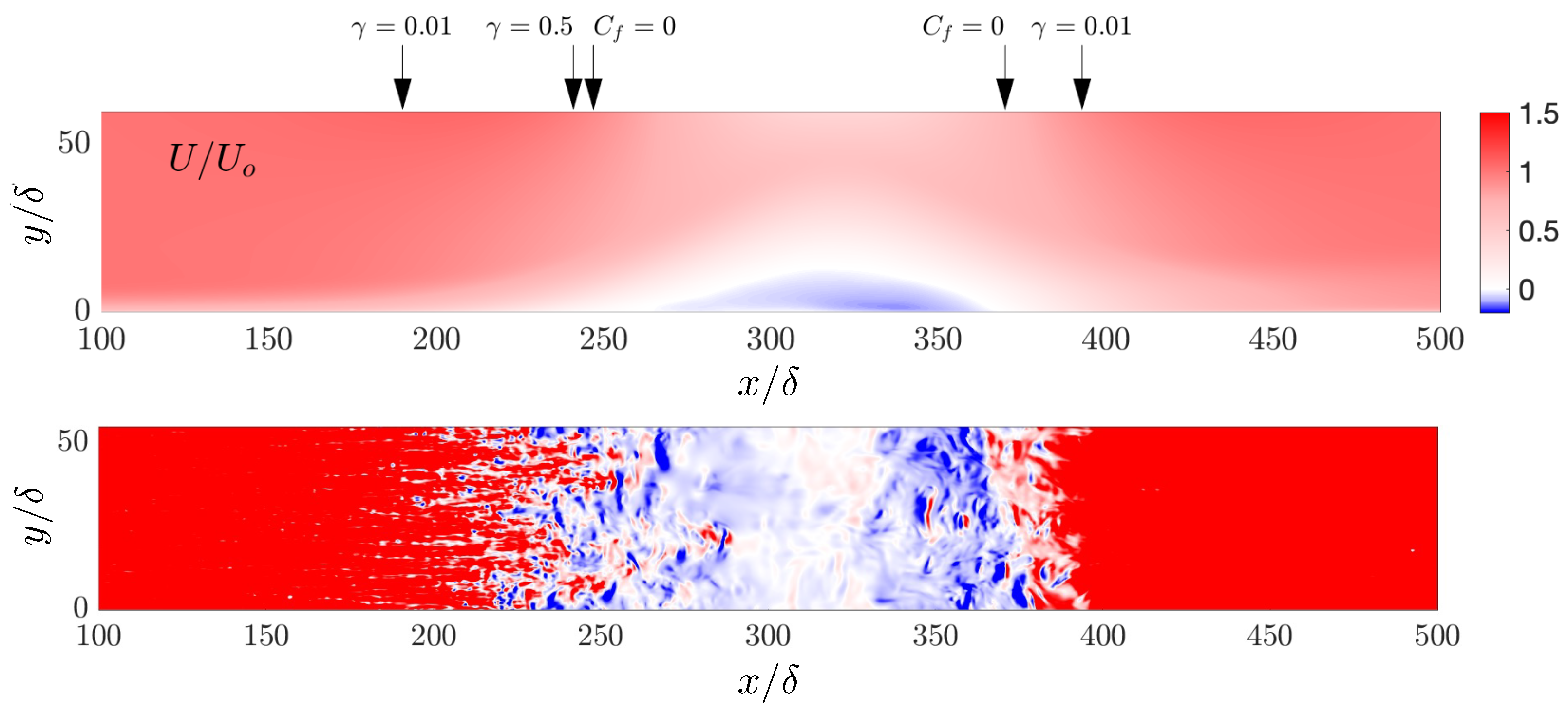
According to Simpson [1], three distinct regions can be identified: (1) intermittent detachment, where instantaneous backflow is present 1% of the time; (2) transitory detachment, where instantaneous backflow is present 50% of the time, and (3) detachment, which occurs on a smooth surface when the time-averaged wall shear stress is zero. Figure 1 shows time-averaged streamwise velocity contours and instantaneous contours of skin-friction coefficient to highlight the various regions. The instantaneous contours, in particular, show the complexity of the phenomenon: regions of backflow appear well ahead of the detachment point, and regions of fluid move downstream well after it. The same phenomena are observed at reattachment.
The structure of separated turbulent flows is drastically different than that of attached flows; in separated flows, for instance, the largest turbulent stresses occur in the center of the separated shear layer. These stresses are mostly caused by large-scale structures generated in the shear layer, which later impinge on the wall in the reattachment region, also causing significant pressure fluctuations there [5]. In separated flows, there is significant interaction between the pressure and velocity fluctuations as the backflow is re-entrained into the outer-region flow [4].
In addition to the inherent unsteadiness of turbulent flows, when separation is present, coherent vortices are shed from the separation point, supplying an additional source of unsteadiness. Another source of unsteadiness may be due to the boundary conditions, which may be time-dependent, as would be the case for a pitching airfoil. In the following, when we refer to “unsteady separation” we will imply that the unsteadiness is of this type.
1.2. Literature Review
Many studies have considered separated flows that are steady in the mean, although in some cases, time-accurate calculations have been carried out that allowed to capture the unsteadiness due to the shedding [9,10,11,12]. In nature, however, pressure gradients are often both space- and time-dependent, for instance, in helicopter and turbomachinery, pitching airfoils, and in the motion of aquatic animals. In these cases, the separation process is unsteady in the mean, and the physical behavior is completely different from the steady counterpart. This literature review concentrates on flows of this type, in which the boundary conditions vary with time.
The imposed unsteadiness can be characterized by the reduced frequency k [13]
where , , and are characteristic length and velocity scales, respectively, and T is the period. The reduced frequency represents the ratio between the convective and unsteady timescales [14]. The response of the flow to the unsteadiness is greatly dependent on k. Leishman [15] identified threshold values to describe unsteadiness in his work on helicopter aerodynamics. A reduced frequency corresponds to a steady flow. The flow is quasi-steady for ; acceleration effects are insignificant, and the ensemble-averaged velocity profiles do not differ from a corresponding steady case. As the reduced frequency grows, acceleration effects begin to dominate the flow characteristics. The threshold values discussed by [15] depend of course on the definition of k; in some problems (pitching airfoil, for instance), and can be unequivocally identified as the freestream velocity and the chord length. In other cases, some ambiguity remains: in rotor dynamics, for instance, the freestream velocity changes continuously along the blade. Specific threshold values of the reduced frequencies are, therefore, not universal.
The body of literature on unsteady boundary layer separation is not as rich as that for steady pressure-gradient distributions; however, starting in the late 1950s, scientists tried to introduce unsteadiness in the flow and observe the impact on the near-wall physics. Most of the time, this was done by prescribing an oscillating freestream perturbation which allowed to modulate the magnitude of the APG felt by the near-wall flow.
A pioneering study on the unsteady APG turbulent boundary layer over a NACA0012 airfoil was carried out by Covert and Lorber [16]. In contrast to previous studies that indicated that the time-averaged profile was nearly independent of the frequency of the freestream oscillation [17,18,19], Covert and Lorber [16] showed that, as the strength of the APG increased, the mean velocity profile assumed an inflectional behavior. These findings were corroborated by Schatzman and Thomas [14], who developed a novel experimental technique to investigate unsteady APG turbulent boundary layers. They also showed that, for an APG strong enough to cause an inflectional velocity profile, the physics of the near-wall flow were dominated by the existence of an embedded shear layer within the boundary layer caused by an inflectional instability mechanism.
The separated shear layer and its associated recirculation bubble play an important role in the dynamics of unsteady separated flows. In a transient separation process, for instance, shedding of the separation region may occur, and the separation bubble may be advected downstream as a solid body. This behavior was observed in backward-facing steps [20], stalled diffusers [4], and, most importantly, in airfoils under dynamic stall conditions, in which a large leading-edge vortex is formed and quickly advected over the chord length of the airfoil [15].
With the increasing power of modern computers, dynamic flow separation was investigated also via numerical simulations. The advection of the recirculation region was observed by Wissink and Rodi [21], who performed large-eddy simulations (LES) of a laminar separation bubble under the effect of an oscillating external flow. Ambrogi et al. [8] examined a turbulent boundary layer subjected to an unsteady freestream APG strong enough to cause separation. They studied a range of frequencies, and observed hysteresis effects that were confined to a thin region near the wall at high frequencies, but extended away from the wall for lower values of k. They further investigated the shedding of the recirculation region [22] which they found was associated with the entrainment of near-wall fluid with high turbulent kinetic energy (TKE) into the shear layer, which led to the persistence of this shear layer as it was advected downstream.
For both DNS and wall-resolved LES, very fine grids and significant computational resources are needed, which makes these techniques unsuitable for industrial applications requiring rapid turnaround. In these cases, the solution of the Reynolds-averaged Navier–Stokes (RANS) equations with turbulence models is prevalent. Turbulence models, however, are not always accurate in separated flows. Even when the separation line is fixed by the geometry (as is the case in the backward-facing step), most models have difficulties predicting the reattachment length (Wilcox [23]). When structural features play a large role (the separated shear layer, or the advection of the separated-flow region, for instance), such models are further challenged, and their accuracy may be expected to be poorer. Although many studies have evaluated the performance of RANS models in steady separation, fewer investigations have considered the unsteady case (unsteady, as mentioned before, in the sense that the boundary conditions—e.g., the freestream pressure gradient—are time-dependent).
The most common turbulence models have been considered, such as the one-equation Baldwin–Barth [24] and Spalart–Allmaras [25] (SA) models, the two-layer model [26], and the two-equation SST model [27]. Configurations studied included airfoils (Ekaterinaris and Menter [28]), flat plates and turbine blades (Nürnberger and Greza [29], Schobeiri and Abdelfattah [30]), and backward-facing steps (Garnier et al. [31]). General conclusions are that the prediction of the hysteresis loop for lift and drag coefficients is incorrect due to errors in the prediction of the separation point [28], that the reattachment point and the size of the separation bubble may also be predicted incorrectly [29,31], and that the return to equilibrium is incorrect [29]. Schobeiri and Abdelfattah [30] attributed these errors to the modeling of the dissipation equation, and to inaccurate transition models.
A drawback of studies that attempt to evaluate turbulence models in non-equilibrium flows is the fact that numerous sources of error are present. In many cases, it is difficult or impossible to separate the modeling errors from numerical ones due to the grid resolution or numerical method, differences in the boundary conditions, or experimental errors. A recent study Park et al. [32] (hereafter referred to as PHY21) tried to overcome this limitation by investigating a flat-plate turbulent boundary layer under unsteady APGs to evaluate the performance of the [27] and SA [25] turbulence models in unsteady separated flows. The numerical setup of their calculations was based on that used by Na and Moin [5]: an APG was generated by applying a profile of freestream wall-normal velocity at the top of the domain, whose amplitude varied in time to obtain dynamic separation and reattachment in the flow. They compared the DNS data with the results from unsteady RANS (URANS) calculations with the models mentioned above. Although they tried to make the numerical methods used for DNS and URANS as similar as possible, some differences remained (and will be mentioned later). PHY21 observed that the turbulence models could predict the formation of the separation bubble and the phase response of the shear layer qualitatively well. However, the phase response of the skin-friction coefficient (and, therefore, the separation and reattachment) was inaccurate: URANS predicted an earlier separation point and a longer recirculation bubble than the DNS. They attributed the near-wall errors in the RANS predictions to the anisotropy of the Reynolds stress.
1.3. Objectives
This work aims at evaluating consistently the capabilities of the three most commonly used one- and two-equation turbulence models to predict unsteady flow separation in a turbulent boundary layer, taking advantage of the simulations recently carried out by Ambrogi et al. [8,22]. The physical phenomena observed by these authors and described above are expected to be difficult to model, making these configurations challenging test cases. Using these data as a reference, furthermore, gives us a unique opportunity to isolate modeling errors. The URANS can be performed using the same numerical methods and boundary conditions, and a grid that, in the LES, gave converged results (in fact, the present URANS are carried out using the same code as the LES, in which the subgrid-scale model is replaced by one of the turbulence models examined). PHY21 were the first that tried to perform this type of evaluation, but they matched the numerical schemes and grid imperfectly, and they considered only one frequency and a single pressure distribution. In our work, we examine three frequencies and three pressure distributions, as well as an additional model (the model). This allows us to evaluate the modeling errors for a wider range of applications. Note that the physical configuration of the problem investigated (a flat-plate boundary layer in a time-varying pressure gradient) is simpler than most of the geometries discussed above. However, the physical phenomena present here are also present in many more complex configurations (as discussed in Refs. [8,22]); for this reason, the present setup has been used in numerous studies of separated flows [5,32,33]. The use of a simpler geometry, furthermore, allows us to compare the URANS results with those of a high-fidelity LES in a rigorous manner, which is the final objective of this study.
The remainder of this article is organized as follows: first, we introduce the problem formulation, including the governing equations, boundary conditions, turbulence models, details on the numerical simulation and the temporal variations of the various cases studied. Then, the results of the RANS calculations are presented and compared to the high-fidelity simulations. Conclusions and recommendations for future work will close the article.
2. Methodology
2.1. Governing Equations
In this study, we solve the phase-averaged equations of conservation of mass and momentum for an incompressible flow:
where are the Cartesian coordinates (we also use x for the streamwise and y for the wall-normal direction) and (or u and v) the velocity components. Phase-averaged quantities are denoted by angle brackets or capital letters, and are defined as
where T is the period of the forcing. A prime indicates the fluctuation around the phase-averaged value: .
The phase-averaged Reynolds stresses are parameterized using an eddy viscosity model:
where is the eddy viscosity, and the rate-of-strain tensor.
Three models in their standard formulations are used: the Spalart–Allmaras (SA) model [25], the SST model [27], and the two-layer formulation of the model [34]. The SA model [25] solves transport equations for a modified eddy viscosity, which was derived using physical considerations and dimensional arguments. The two-layer model [34] solves transport equations for the turbulent kinetic energy (TKE) and for the dissipation of TKE, . The eddy viscosity is then given by , where is a constant. In the near-wall region, the equation for is not solved, and algebraic expressions are used to determine a length scale. The SST model [27] solves transport equations for the TKE and for the turbulent frequency ; the eddy viscosity , where is a limiter that avoids the over-estimation of the shear stresses. The standard forms of the model described in the papers cited are used.
Numerical integration of Equation (2) is performed using second-order-accurate central differences on a staggered mesh. A second-order-accurate semi-implicit time advancement is used, with a Crank–Nicolson scheme for wall-normal diffusive terms and a low-storage third-order Runge–Kutta scheme for the others. The equations are advanced in time using the fractional-step method [35,36]. The Poisson solver uses a Fourier decomposition in x and direct inversion of the resulting tridiagonal matrices. The code has been validated extensively and previously applied to similar problems [7,37,38].
2.2. Problem Formulation
We replicate the problem studied by Ambrogi et al. [8]; the computational domain, however, is two-dimensional. We consider a spatially developing turbulent boundary layer on a flat plate; the geometry is shown in Figure 2. The LES used a three-dimensional domain of dimensions , where is the displacement thickness at the inflow, significantly longer than that used in other calculations [5,6]. The present simulation uses a 2D domain whose length and height match those of the LES. The mesh for the URANS calculations has grid points; this resolution was chosen based on the grid-convergence study of Ambrogi et al. [8], whose production runs were carried out on a fine grid using points, but had obtained grid convergence using point; we chose the latter resolution, which is, in any case, much finer than what would be typical in a URANS simulation. The Reynolds number, based on and the freestream velocity at the inlet, , is . Based on the friction velocity at the inlet, the grid size in wall units is , . The calculations were carried out in time-accurate mode, and the CFL number did not exceed 0.5.
A no-slip condition is applied at the wall, and a convective condition is used at the outflow [39]. At the inflow, the LES used a sequence of -planes obtained from separate simulations. We followed the same approach, using, however, the phase-average of the LES data. For the turbulent quantities, and could be calculated directly from the LES, while for the model, the eddy viscosity was first computed as
and the turbulent frequency was then obtained as .
The freestream pressure gradient is generated by imposing an unsteady vertical-velocity distribution on the upper side of the domain. The wall-normal velocity is given by
where , , , and . The spatial variation matches the suction-blowing velocity profile used by [5]. Let be the phase angle. Three periodic temporal-variation laws were used:
The streamwise velocity component was then obtained by imposing zero spanwise vorticity. In Case A, an FPG precedes an APG for , while the APG precedes the FPG in the reset of the cycle. The separation occurs only around . At and the freestream pressure gradient is nearly zero. In Case B, on the other hand, the APG always precedes the FPG, and the flow is separated throughout the cycle. This distribution matches the one by Park et al. [32]. In Case C, finally, the APG also precedes the FPG, but at and , generating a nominally ZPG boundary layer. Figure 3 shows the streamwise and wall-normal freestream-velocity profiles for the three cases.
We define the reduced frequency as , where is the length over which the pressure gradient varies, and . was chosen by analogy with pitching airfoils, in which would be the chord length. In Case A, three values of k were used: , 1, and 10. Steady calculations were also performed with corresponding to the and , and phases. For , the flow is quasi-steady, as the convective time scale is much lower than the imposed unsteady time scale. In the case, the two scales are similar. Finally, the high-frequency case corresponds to a flutter-like rapid oscillation.
3. Results
3.1. Effect of Reduced Frequency
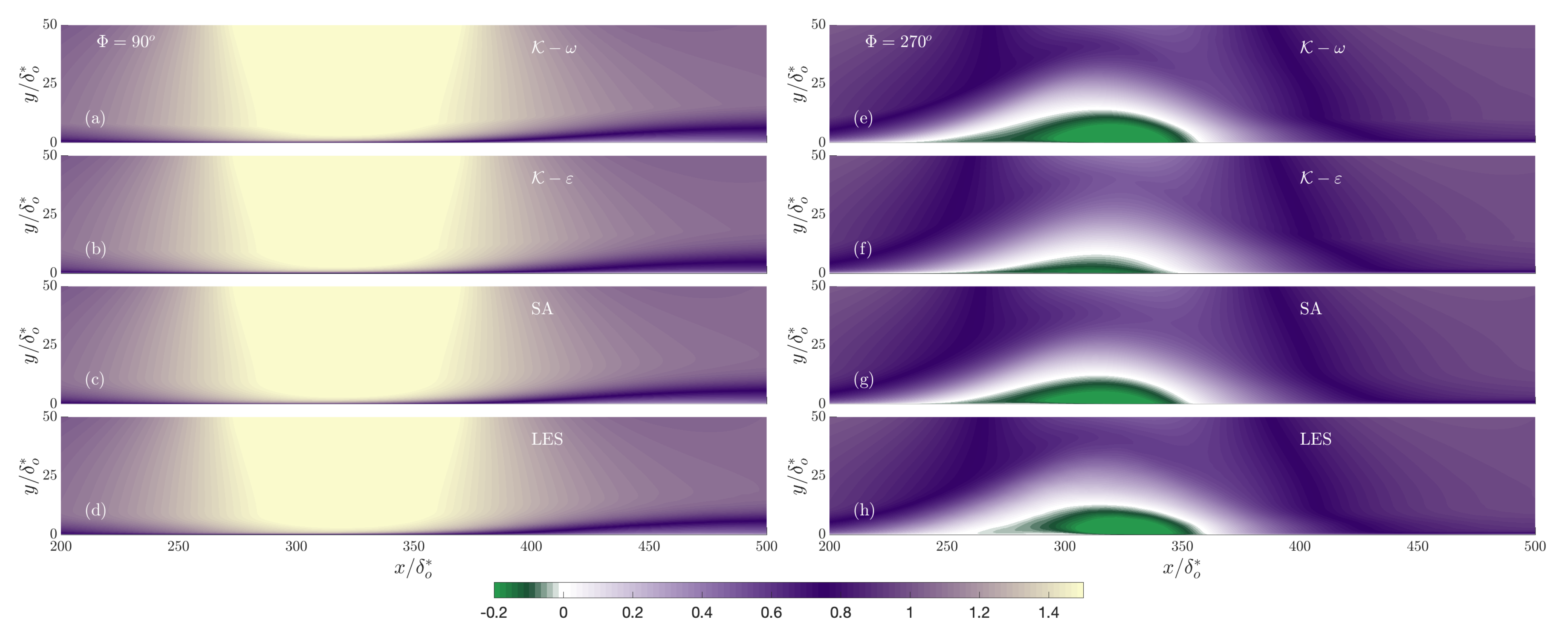
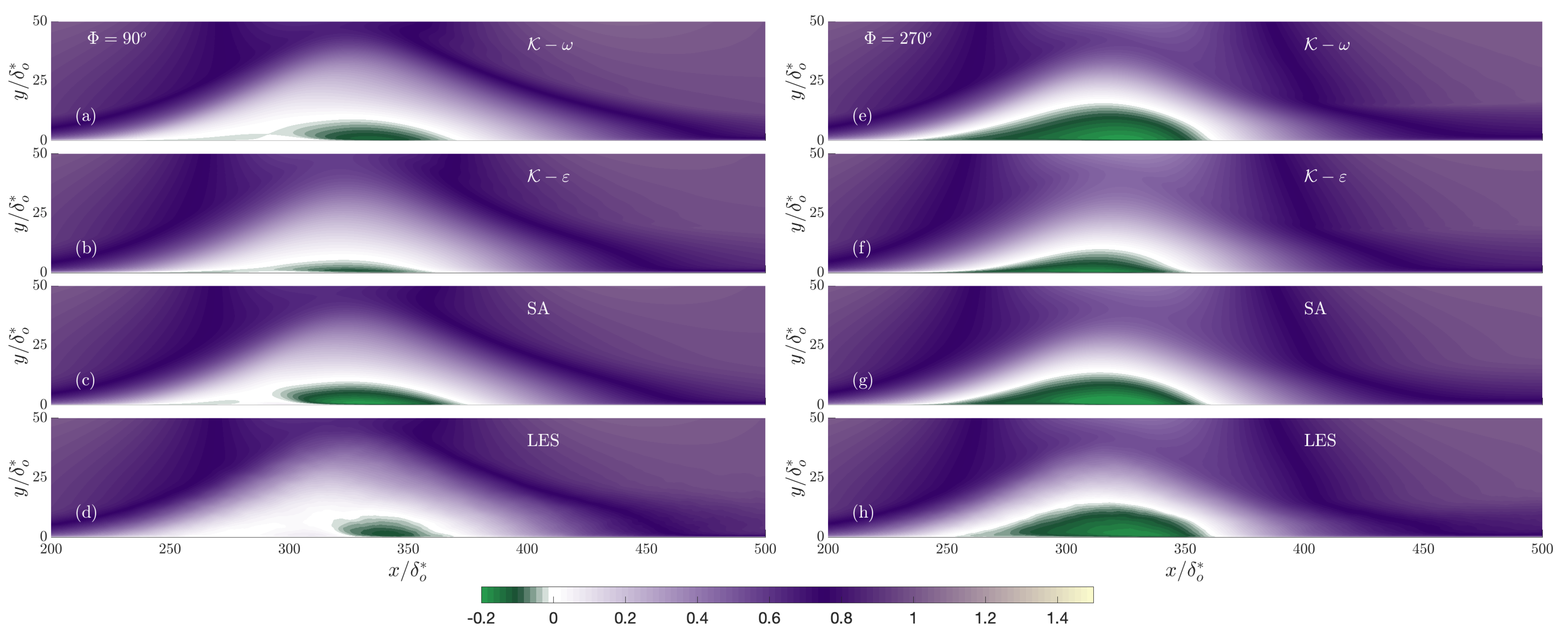
The phase-averaged data were collected at 20 equispaced phases, . Figure 4, Figure 5 and Figure 6 show contours of the phase-averaged streamwise velocity at two phases of the cycle. At , the strongest FPG is followed by the strongest APG, whereas at , the FPG follows the APG. In all cases, at , the boundary layer is thinned in the accelerating-flow region where , (i.e., ). At , the APG causes separation, and a recirculation bubble is formed; the flow then reattaches in the FPG region. The height of the bubble is minimum at high frequency and largest at the lowest one. At the intermediate frequency, the recirculation bubble is advected downstream, almost as a solid body (see [22] for a discussion of the causes of this phenomenon). At , the advected region is exiting the domain.
Each turbulence model predicts the general features of the flow with only small discrepancies from the LES. The downstream shedding of the recirculation region and the reattachment of the boundary layer are complex phenomena, and the fact that the model can capture them is important (and, perhaps, unexpected). Small discrepancies between the models are observed in the size and shape of the shed region, but the general features of the flow are correct.
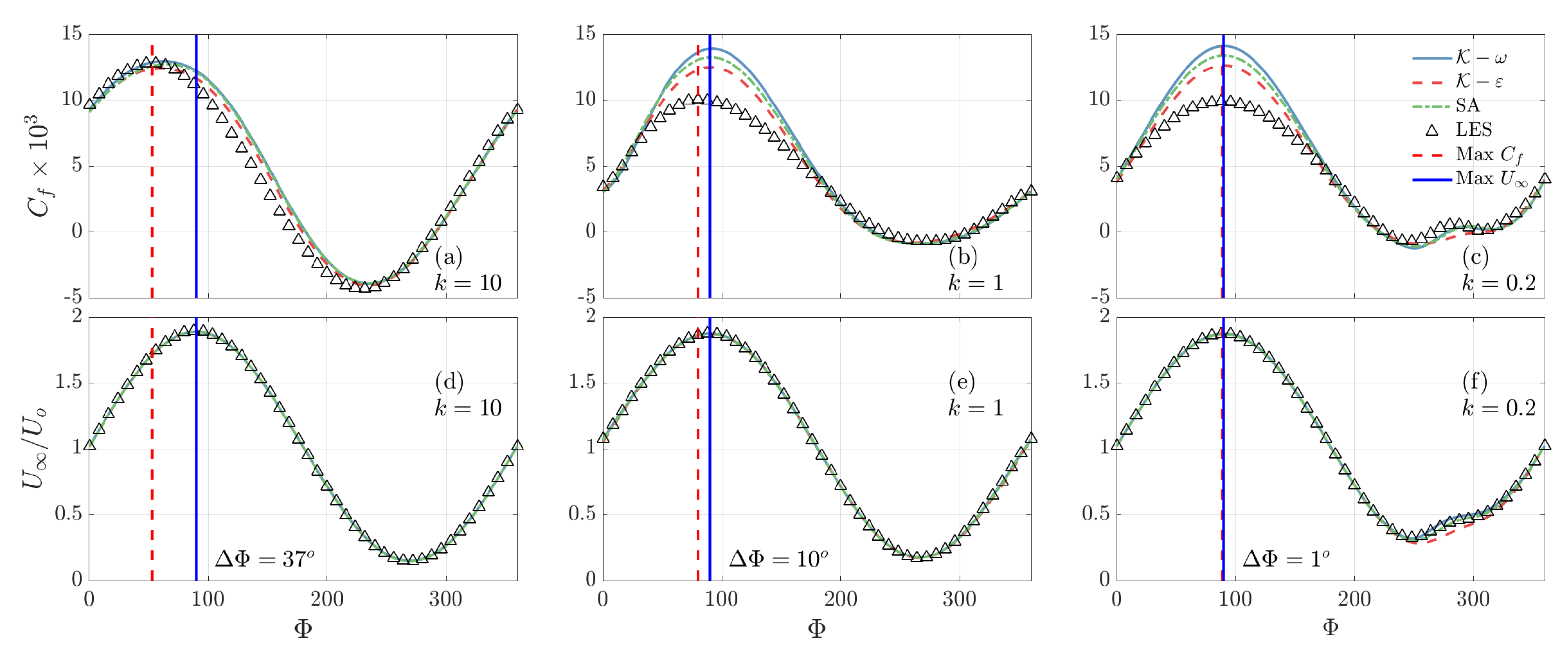
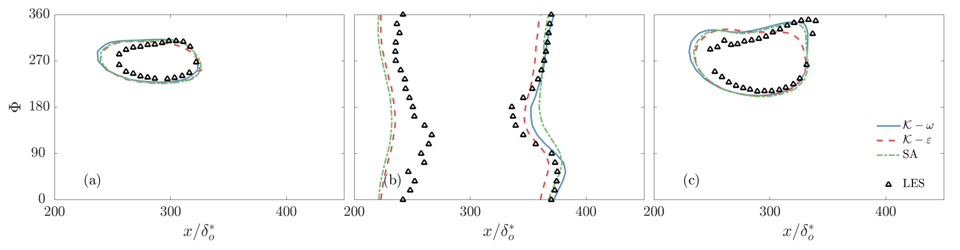
Figure 7 shows the skin-friction coefficient at four phases of the cycle. Note that at , a phase shift is observed between the forcing and the flow response, to be discussed below, so different phases were chosen compared with the other cases. At the high frequency, the agreement is very good, except at , towards the middle of the deceleration part of the period. During this phase, the skin-friction coefficient is consistently over-predicted, indicating that the model does not respond quickly enough to the very rapid change of the forcing. The fact that all models respond in a similar way indicates that this issue is not due to the particular choice of the time scale of each model, but rather to some more fundamental model assumption (such as, for instance, the eddy viscosity assumption) and the fact that these models are calibrated in equilibrium boundary layers. Figure 8 shows the skin-friction coefficient and the freestream velocity at the center of the recirculation region. The maximum and minimum skin-friction precedes the maximum and minimum freestream velocity by . This is consistent with the overall behavior of the flow at this frequency, which exhibits a decoupling between the inner and outer layer, similar to that observed in Stokes’ second problem, the oscillating plate (which has a phase shift of ). This issue is also discussed by [8]. The dimensions of the recirculation region, Figure 9a, are predicted quite accurately at this frequency and at the intermediate one, although in the latter case, separation is predicted to occur earlier both in space and time. At the lowest frequency, errors are more significant, especially in the prediction of the separation point. In general, the longer the period, the larger the error for these quantities. At high and intermediate frequencies, the fact that the flow goes through two ZPG phases (for which the models are calibrated) tends to limit the divergence of the model solution from the correct one. At low frequency, on the other hand, the flow field has more time to respond to the model (mis)prediction, and thus errors are increased.
At the intermediate and low frequencies, Figure 7f–l, the error is greatest in the FPG phases (). This is expected, since in FPG flows, the coherent-eddy structure changes significantly, as the streamwise vortices become more elongated and the correlation between and fluctuations decreases [40]. This type of phenomenon is difficult to reproduce using turbulence models, which are best at predicting shear-driven flows. In fact, the turbulence models significantly overpredict the Reynolds shear stresses, Figure 10, a result consistent with that of [32]. At these frequencies the phase shift between and decreases (Figure 8). At , the agreement between models and LES during separation is remarkably good, better than for a steady case. At the low frequency, the agreement is at least as good as in the steady case. Note that during the FPG phases, the is the most accurate model, while in the separation phases, gives the best results. SA is always in-between those.
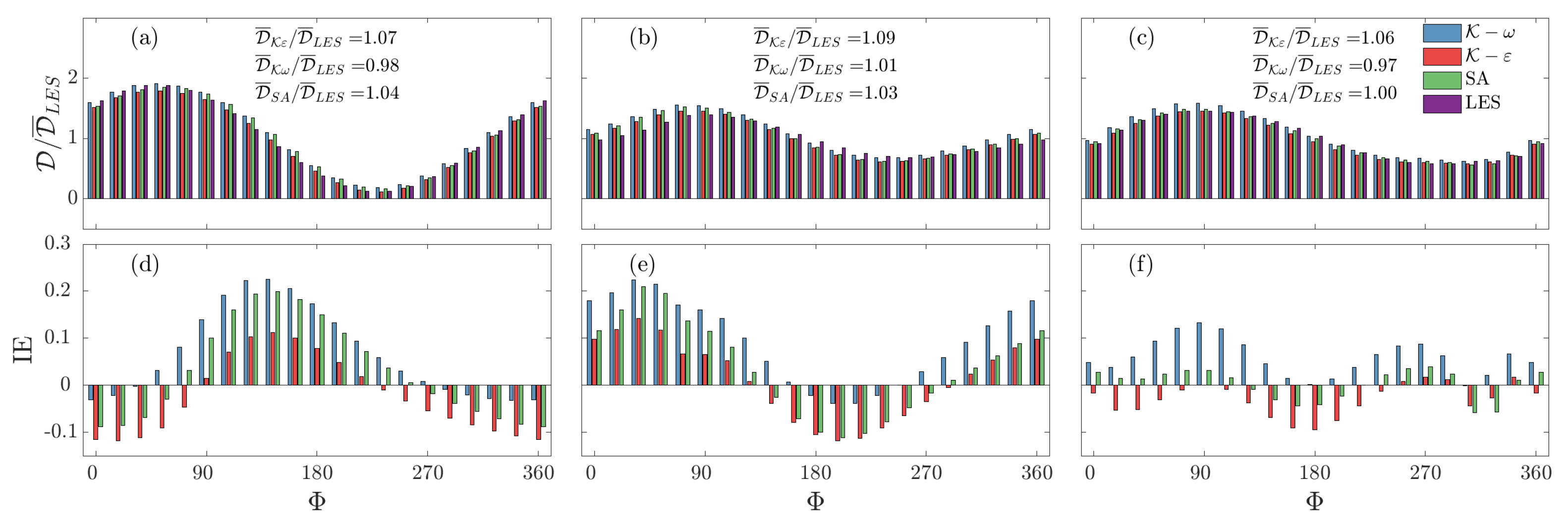
A quantity that is of primary interest to engineers is the drag. We calculated it by integrating the skin-friction coefficient over the region where the pressure gradient is significant, extending to the outflow. Including the upstream regions, in which the flow remains ZPG throughout the cycle, would artificially decrease the difference between the model results and the LES, since in that region, all the models are accurate. The integration, however, is carried out all the way to the outflow (where is stationary) to account for the passing of the shed recirculation zone. We also defined an integral error as the difference between the model prediction and the LES result, this error is normalized by the time-averaged drag from the LES:
The drag (normalized by ) and the integral error are shown in Figure 11. The drag prediction is quite accurate, partly because of error cancellation (see, for example, the distribution in Figure 7f,j, in which the overprediction of the skin-friction at is partially balanced by its underprediction further downstream). Apart from the strong acceleration phases, the error is 10% or below for the intermediate and low frequencies. The time-averaged drag is also predicted quite accurately at those frequencies (within 6% of the LES value), although, again, error cancellation contributes to this result.
3.2. Effect of Pressure Distribution
We next studied two additional cases in which the spatial distribution was unchanged, but two different temporal modulations were assigned, as discussed in the Introduction (Section 1). They are referred to as Cases B and C, respectively, and the freestream velocities corresponding to each case are shown in Figure 3. Physically, Case A may represent the flow of an airfoil pitching between angles of attack and , Case B mimics an airfoil pitching between two angles of attack and , and Case C an airfoil pitching between angles of attack 0 and . In all cases examined in this section, the reduced frequency is . Apart from the Reynolds number, which is substantially higher (), and for the domain size (which is, in the present simulations, longer), Case B is identical to the flow studied by [32].
Figure 12 and Figure 13 show contours of the phase-averaged streamwise velocity for Cases B and C. For Case A, the contours were shown in Figure 5. In Case B, the recirculation bubble persists throughout the cycle, although it is modulated by the time-varying blowing/suction profile, as can also be seen in Figure 14. In Case C, the recirculation bubble is somewhat larger than in Case A (reflecting the fact that the APG is present (at different strengths) throughout the entire cycle. The early separation observed by [32] is observed here, not only in Case C, but in the other ones as well. The reattachment, however, is predicted more accurately.
The skin-friction coefficient distribution for cases A, B, and C is shown in Figure 15 For Case B it has a distribution very similar to the steady or low-frequency cases, and is predicted less accurately than in the case. The in the separation region is, once again, predicted more accurately in the unsteady cases A and C than in the quasi-steady, low-frequency, one. In Cases B and C, the least accurate prediction occurs in the recovery region after reattachment. In that region, the Reynolds shear stresses (Figure 16) are significantly underpredicted, and the underestimation of the turbulent mixing leads to the slower recovery.
Despite the errors in , the phase-averaged drag is predicted with the same level of accuracy observed before, and is close to the LES result. The only exception is Case B (the one with separation throughout the cycle), in which the error can be as high as 9% (for the SA model).
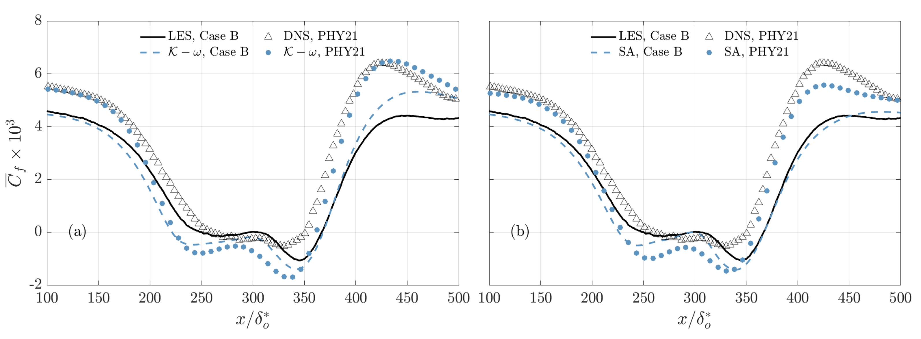
Finally, in Figure 17, we compare the DNS and RANS calculation results by [32] with the present LES, and our model results. The higher Reynolds number results in lower , in our case, in the inlet section. A notable feature of this figure is the fact that the modeled calculations in PHY21 resemble more, in shape, the present calculations than the DNS. In particular, the two-lobed structure of the recirculation region, present at the higher , is also observed in the model predictions in PHY21. We conjecture that the differences in numerics and grid resolution play a role here. PHY21 carried out their URANS simulations using OpenFOAM [41], on a grid significantly coarser than the DNS one. Although the authors attempted to use the same scheme for the URANS and DNS, the URANS used a co-located method, while the DNS used a staggered grid. While the staggered grid conserves momentum and energy discretely, the co-located scheme is not energy conserving, even with the parameters used [42]. We conjecture that the more significant errors observed by PHY21 are not due exclusively to the turbulence model, as they argue, but rather to a combination of turbulence modeling inaccuracies and numerical errors due to the different grid resolution and grid-point arrangement (staggered vs. co-located) that results in excessive numerical diffusion.
4. Summary and Conclusions
We performed simulations of a flat-plate turbulent boundary layer subjected to a time-varying freestream pressure distribution that resulted in unsteady separation. The results of five wall-resolved large-eddy simulations (WRLES) [8] were used to evaluate the accuracy of three commonly used turbulence models for the solution of the unsteady Reynolds-averaged Navier–Stokes (URANS) equations, namely the – SST model [27], the two-layer – model [34], and the Spalart–Allmaras model [25].
In most evaluations of turbulence models, discrepancies between model predictions and reference data can be due to a variety of sources: numerical resolution, errors due to the specific discretization used, differences in boundary conditions, and uncertainties in the reference data. The novelty of the present study lies in the fact that, by performing the URANS simulations using the same numerical method and boundary conditions as the WRLES, and a grid on which converged results were obtained by the WRLES, we were able to isolate the modeling errors. We performed two sets of comparisons: first, for a given freestream pressure distribution we considered various frequencies. Then, we kept the frequency constant and varied the unsteady pressure distribution.
In the first set of calculations, the freestream pressure (which was always imposed by a suction/blowing profile at the freestream) varied symmetrically between a favurable pressure gradient (FPG) and an adverse pressure gradient (APG), so that separation occurred during part of the cycle only, and the flow passed through two phases in which the pressure gradient was zero (ZPG). Three frequencies were considered. Next, we considered a case (Case B) corresponding to the study of Park et al. [32], in which the flow was separated throughout the cycle, and one (Case C), in which the APG always preceded the FPG in space, and the magnitude of the pressure gradients was varied in time, reaching a ZPG phase.
The main results of this study were:
- The turbulence model’s accuracy is comparable for the three models considered. They uniformly predict early separation, and the length of the recirculation region is generally overestimated.
- At the intermediate frequency, all turbulence models predict the downstream advection of the recirculation region that was observed in the resolved LES.
- The mean velocity profiles are reasonably accurate in the outer layer, the errors being concentrated in the near-wall region, especially near the separation and reattachment points.
- The Reynolds shear stresses are over-predicted during the acceleration phases, as observed previously [32].
- The drag is predicted with good accuracy, the integrated error (IE) remains always below 10% for all models.
- The results of Park et al. [32] resemble qualitatively our results, but the error there is larger. We conjecture that the error, in this case, is due to a combination of factors. In particular, the more dissipative character of the numerical method used for the RANS calculations, coupled with the coarser grid used, could result in additional diffusion. In our case, numerical errors were the same for the RANS calculations and the LES.
It should be remarked that our simulations used a grid much finer than those typically used in RANS calculations, and, furthermore, that industrial codes resemble OpenFOAM more than our staggered method. In a practical calculation, therefore, the error would be higher. Our calculations, however, are useful in that they point out that the turbulence models are responsible only for part of the discrepancies, and that other aspects of the calculations (and not only the turbulence models) must be improved in order to achieve greater fidelity.
Future work could follow various routes. One of them is the inclusion of roughness, which substantially changes the dynamics of separation [7]. Roughness modifications for RANS models have been developed and calibrated mostly in equilibrium flows, and their accuracy decreases near separation. Since most real surfaces are rough, the accuracy with which RANS models with roughness modifications can predict the flow is critical for applications in engineering and in the natural sciences. Another important aspect that should be addressed in future studies is the presence of curvature, both in the streamwise and in the lateral (z) direction. Even weak curvature affects the shear stresses significantly [43], and eddy viscosity models must be modified to include these effects (see Spalart and Shur [44], and the discussion by Durbin and Pettersen-Reif [45]). Verifying whether these modifications give accurate results when unsteady separation is present would also help set error bars for the use of turbulence models in realistic industrial applications.
Supplementary Materials
The following supporting information can be downloaded at: https://www.mdpi.com/article/10.3390/fluids8100273/s1.
Author Contributions
C.Y.M. was the primary author, planned and performed the numerical simulations, and interpreted the results. U.P. and F.A. contributed to the idea, the data interpretation, and discussion. All authors commented on the manuscript and provided editorial assistance. All authors have read and agreed to the published version of the manuscript.
Funding
Research supported by the Natural Science and Engineering Research Council of Canada (NSERC) and Hydro Québec under CRD grant CRDPJ 514642-17. Computational support provided by the Digital Research Alliance of Canada.
Data Availability Statement
The data presented in this study are available on request from the corresponding author.
Conflicts of Interest
The authors declare no conflict of interest.
References
- Simpson, R.L. Review—A Review of Some Phenomena in Turbulent Flow Separation. J. Fluids Eng. 1981, 103, 520–533. [Google Scholar] [CrossRef]
- Perry, A.E.; Fairlie, B.D. A study of turbulent boundary-layer separation and reattachment. J. Fluid Mech. 1975, 69, 657–672. [Google Scholar] [CrossRef]
- Patrick, W.P. Flowfield Measurements in a Separated and Reattached Flat Plate Turbulent Boundary Layer. Final Report; NASA contractor report NASA-CR-4052; National Aeronautics and Space Administration: Washington DC, USA, 1987. [Google Scholar]
- Simpson, R.L. Turbulent Boundary-Layer Separation. Annu. Rev. Fluid Mech. 1989, 21, 205–232. [Google Scholar] [CrossRef]
- Na, Y.; Moin, P. Direct numerical simulation of a separated turbulent boundary layer. J. Fluid Mech. 1998, 370, 175–201. [Google Scholar]
- Abe, H. Reynolds-number dependence of wall-pressure fluctuations in a pressure-induced turbulent separation bubble. J. Fluid Mech. 2017, 833, 563–598. [Google Scholar] [CrossRef]
- Wu, W.; Piomelli, U. Effects of surface roughness on a separating turbulent boundary layer. J. Fluid Mech. 2018, 841, 552–580. [Google Scholar] [CrossRef]
- Ambrogi, F.; Piomelli, U.; Rival, D.E. Characterization of unsteady separation in a turbulent boundary layer. J. Fluid Mech. 2022, 945, 1–30. [Google Scholar] [CrossRef]
- Durbin, P.A. Separated flow calculations with the k-ε-v2 model. AIAA J. 1995, 33, 659–664. [Google Scholar]
- Jin, G.; Braza, M. Two-equation turbulence model for unsteady separated flows around airfoils. AIAA J. 1994, 32, 2316–2320. [Google Scholar] [CrossRef]
- Basu, D.; Hamed, A.; Das, K. DES, hybrid RANS/LES and PANS models for unsteady separated turbulent flow simulations. In Proceedings of the Fluids Engineering Division Summer Meeting, Houston, TX, USA, 19–23 June 2005; Paper FEDSM2005-77421. Volume 41995, pp. 683–688. [Google Scholar]
- Hamed, A.; Basu, D.; Das, K. Assessment of multiscale resolution for hybrid turbulence model in unsteady separated transonic flows. Comput. Fluids 2007, 36, 924–934. [Google Scholar] [CrossRef]
- Covert, E.E.; Fletcher, M.J.; Flittie, K.J.; Linton, S.W. On the Unsteady Characteristics of Flows around an NACA 0012 Airfoil; Technical Report; MIT Center for Aerodynamic Studies: Cambridge, MA, USA, 1986. [Google Scholar]
- Schatzman, D.M.; Thomas, F.O. An experimental investigation of an unsteady adverse pressure gradient turbulent boundary layer: Embedded shear layer scaling. J. Fluid Mech. 2017, 815, 592–642. [Google Scholar] [CrossRef]
- Leishman, G.J. Principles of Helicopter Aerodynamics with CD Extra; Cambridge University Press: Cambridge, UK, 2006. [Google Scholar]
- Covert, E.E.; Lorber, P.F. Unsteady turbulent boundary layers in adverse pressure gradients. AIAA J. 1984, 22, 22–28. [Google Scholar] [CrossRef]
- Karlsson, S.K.F. An unsteady turbulent boundary layer. J. Fluid Mech. 1959, 5, 622–636. [Google Scholar] [CrossRef]
- Kenison, R.C. An experimental study of the effect of oscillatory flow on the separation region in a turbulent boundary layer. In Proceedings of the Unsteady Aerodynamics, AGARD Conference Proceedings, Ottawa, ON, Canada, 26–28 September 1977; Volume 227. [Google Scholar]
- Parikh, P.G.; Reynolds, W.C.; Jayaraman, R. Behavior of an unsteady turbulent boundary layer. AIAA J. 1982, 20, 769–775. [Google Scholar] [CrossRef]
- Mullin, T.; Greated, C.A.; Grant, I. Pulsating flow over a step. Phys. Fluids 1980, 23, 669–674. [Google Scholar] [CrossRef]
- Wissink, J.G.; Rodi, W. DNS of a laminar separation bubble in the presence of oscillating external flow. Flow Turb. Combust. 2003, 71, 311–331. [Google Scholar] [CrossRef]
- Ambrogi, F.; Piomelli, U.; Rival, D.E. Characterization of unsteady separation in a turbulent boundary layer: Reynolds stresses and flow dynamics. J. Fluid Mech. 2023, 972, A36. [Google Scholar] [CrossRef]
- Wilcox, D.C. Turbulence modeling: An overview. In Proceedings of the 39th Aerospace Sciences Meeting and Exhibit, Reno, NV, USA, 8–11 January 2001. AIAA Paper 2001-0724. [Google Scholar]
- Baldwin, B.S.; Barth, T.J. A One-Equation Turbulence Transport Model for High Reynolds Number Wall-Bounded Flows. NASA Technical Memorandum TM 102847. Available online: https://arc.aiaa.org/doi/abs/10.2514/6.1991-610 (accessed on 27 September 2023).
- Spalart, P.R.; Allmaras, S.R. A One-Equation Turbulence Model for Aerodynamic Flows. Rech. AÉrospatiale 1994, 1, 5–21. [Google Scholar]
- Patel, V.C.; Yoon, J.Y. Application of Turbulence Models to Separated Flow Over Rough Surfaces. J. Fluids Eng. 1995, 117, 234–241. [Google Scholar] [CrossRef]
- Menter, F.R. Two Equation Eddy Viscosity Turbulence Models for Engineering Applications. AIAA J. 1994, 32, 1598–1605. [Google Scholar] [CrossRef]
- Ekaterinaris, J.A.; Menter, F.R. Computation of oscillating airfoil flows with one- and two-equation turbulence models. AIAA J. 1994, 32, 2359–2365. [Google Scholar] [CrossRef]
- Nürnberger, D.; Greza, H. Numerical investigation of unsteady transitional flows in turbomachinery components based on a RANS approach. Flow Turb. Combust. 2002, 69, 331–353. [Google Scholar] [CrossRef]
- Schobeiri, M.T.; Abdelfattah, S. On the Reliability of RANS and URANS Numerical Results for High-Pressure Turbine Simulations: A Benchmark Experimental and Numerical Study on Performance and Interstage Flow Behavior of High-Pressure Turbines at Design and Off-Design Conditions Using Two Different Turbine Designs. J. Turbomach. 2013, 135, 061012. [Google Scholar] [CrossRef]
- Garnier, E.; Pamart, P.Y.; Dandois, J.; Sagaut, P. Evaluation of the unsteady RANS capabilities for separated flows control. Comput. Fluids 2012, 61, 39–45. [Google Scholar] [CrossRef]
- Park, J.; Ha, S.; You, D. On the unsteady Reynolds-averaged Navier–Stokes capability of simulating turbulent boundary layers under unsteady adverse pressure gradients. Phys. Fluids 2021, 33, 065125. [Google Scholar] [CrossRef]
- Na, Y.; Moin, P. The structure of wall-pressure fluctuations in turbulent boundary layers with adverse pressure gradient and separation. J. Fluid Mech. 1998, 377, 347–373. [Google Scholar] [CrossRef]
- Chen, H.; Patel, V. Near-wall turbulence models for complex flows including separation. AIAA J. 1988, 26, 641–648. [Google Scholar] [CrossRef]
- Chorin, A.J. Numerical solution of Navier-Stokes equations. Math. Comput. 1968, 22, 745–762. [Google Scholar] [CrossRef]
- Kim, J.; Moin, P. Application of a fractional step method to incompressible Navier-Stokes equations. J. Comput. Phys. 1985, 59, 308–323. [Google Scholar] [CrossRef]
- Keating, A.; Piomelli, U.; Bremhorst, K.; Nešić, S. Large-eddy simulation of heat transfer downstream of a backward-facing step. J. Turbul. 2004, 5, 20. [Google Scholar] [CrossRef]
- Yuan, J.; Piomelli, U. Numerical simulation of a spatially developing accelerating boundary layer over roughness. J. Fluid Mech. 2015, 780, 192–214. [Google Scholar] [CrossRef]
- Orlanski, I. A simple boundary condition for unbounded hyperbolic flows. J. Comput. Phys. 1976, 21, 251–269. [Google Scholar] [CrossRef]
- Piomelli, U.; Yuan, J. Numerical simulations of spatially developing, accelerating boundary layers. Phys. Fluids 2013, 25, 101304. [Google Scholar] [CrossRef]
- Weller, H.G.; Tabor, G.; Jasak, H.; Fureby, C. A tensorial approach to computational continuum mechanics using object-oriented techniques. Comput. Phys. 1998, 12, 620–631. [Google Scholar] [CrossRef]
- Morinishi, Y.; Lund, T.S.; Vasilyev, O.V.; Moin, P. Fully conservative higher order finite difference schemes for incompressible flows. J. Comput. Phys. 1998, 143, 90–124. [Google Scholar] [CrossRef]
- Bradshaw, P.; Young, A.D. Effects of Streamline Curvature on Turbulent Flow; Technical Report AGARD-AG-169; AGARD: Paris, France, 1973. [Google Scholar]
- Spalart, P.R.; Shur, M.L. On the sensitization of turbulence models to rotation and curvature. Aerosp. Sci. Technol. 1997, 5, 297–302. [Google Scholar] [CrossRef]
- Durbin, P.A.; Pettersson Reif, B.A. Statistical Theory and Modeling for Turbulent Flows, 1st ed.; Wiley: Hoboken, NJ, USA, 2001. [Google Scholar]
Figure 1.
Detachment of a turbulent boundary layer. is the percentage of backflow (fluid moving upstream): (Top) mean streamwise velocity contours; (bottom) instantaneous contours of the skin-friction coefficient (red: positive; blue: negative. Data from [8].
Figure 1.
Detachment of a turbulent boundary layer. is the percentage of backflow (fluid moving upstream): (Top) mean streamwise velocity contours; (bottom) instantaneous contours of the skin-friction coefficient (red: positive; blue: negative. Data from [8].

Figure 2.
Sketch of the computational setup for LES (left) and URANS (right).

Figure 3.
Freestream velocity distribution. (a–c) ; (d–f) . (a,d) Case A; (b,e) Case B; (c,f) Case C. The gray area is the envelope of the velocity profile through the cycle, while the lines show the four extreme phases.
Figure 3.
Freestream velocity distribution. (a–c) ; (d–f) . (a,d) Case A; (b,e) Case B; (c,f) Case C. The gray area is the envelope of the velocity profile through the cycle, while the lines show the four extreme phases.
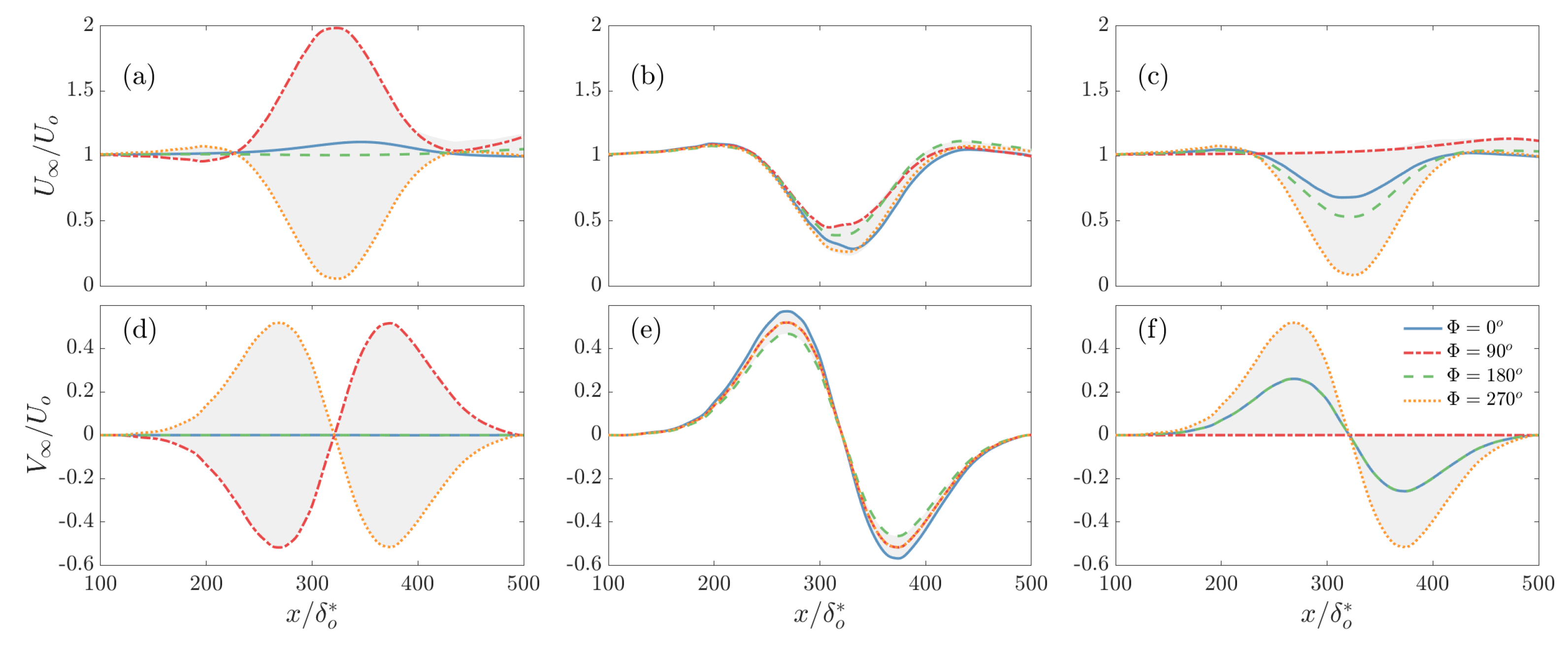
Figure 4.
Contours of the phase-averaged streamwise velocity at (a–d) and (e–h), .
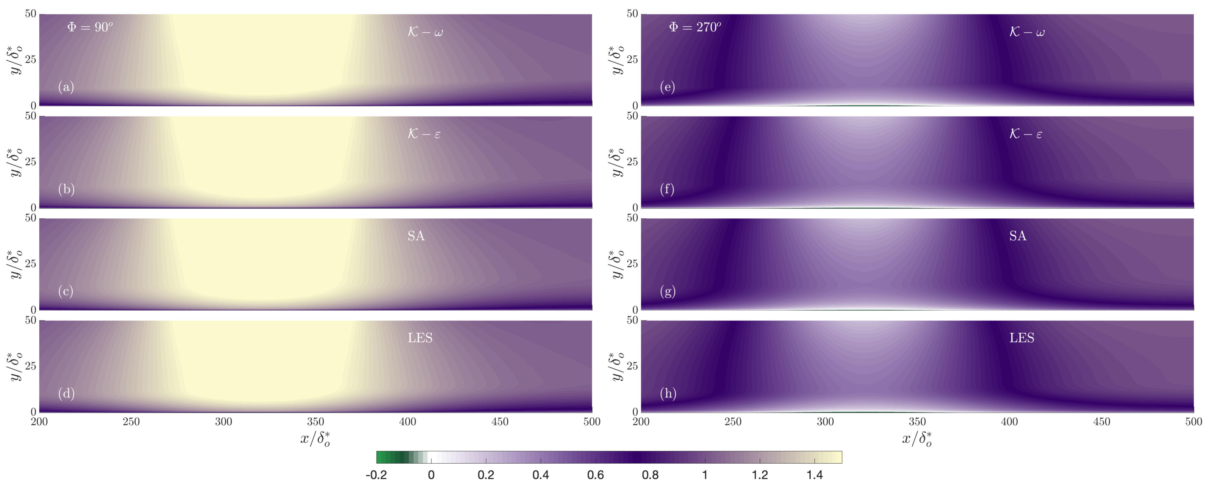
Figure 5.
Contours of the phase-averaged streamwise velocity at (a–d) and (e–h), . The Supplementary Material contains an animation showing the entire cycle (Supplemental File S1).
Figure 5.
Contours of the phase-averaged streamwise velocity at (a–d) and (e–h), . The Supplementary Material contains an animation showing the entire cycle (Supplemental File S1).
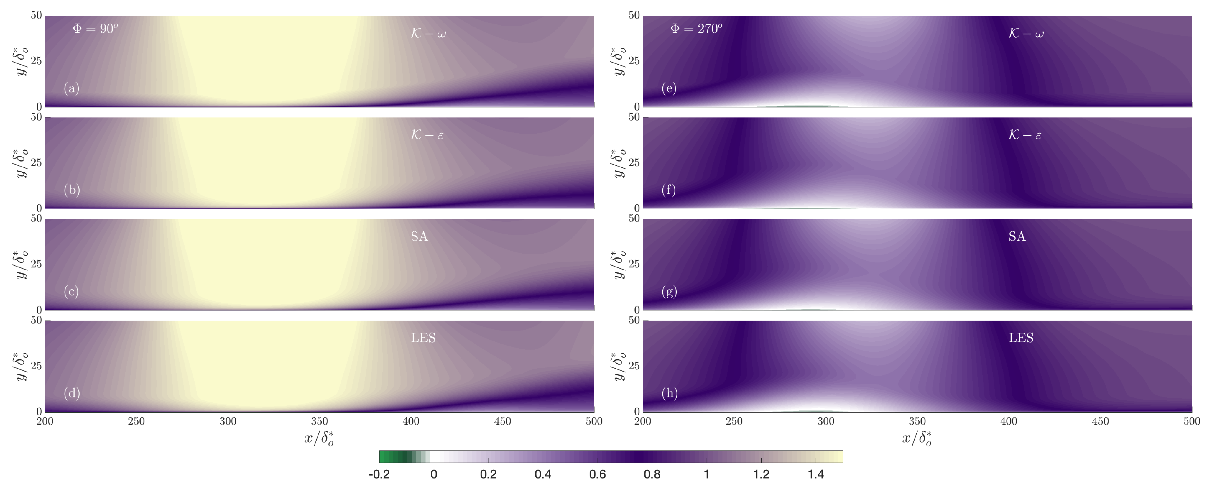
Figure 6.
Contours of the phase-averaged streamwise velocity at (a–d) and (e–h), .

Figure 7.
Skin-friction coefficient at four phases in the cycle. (a–d) ; (e–h) ; (i–l) ; (m–p) steady.
Figure 7.
Skin-friction coefficient at four phases in the cycle. (a–d) ; (e–h) ; (i–l) ; (m–p) steady.
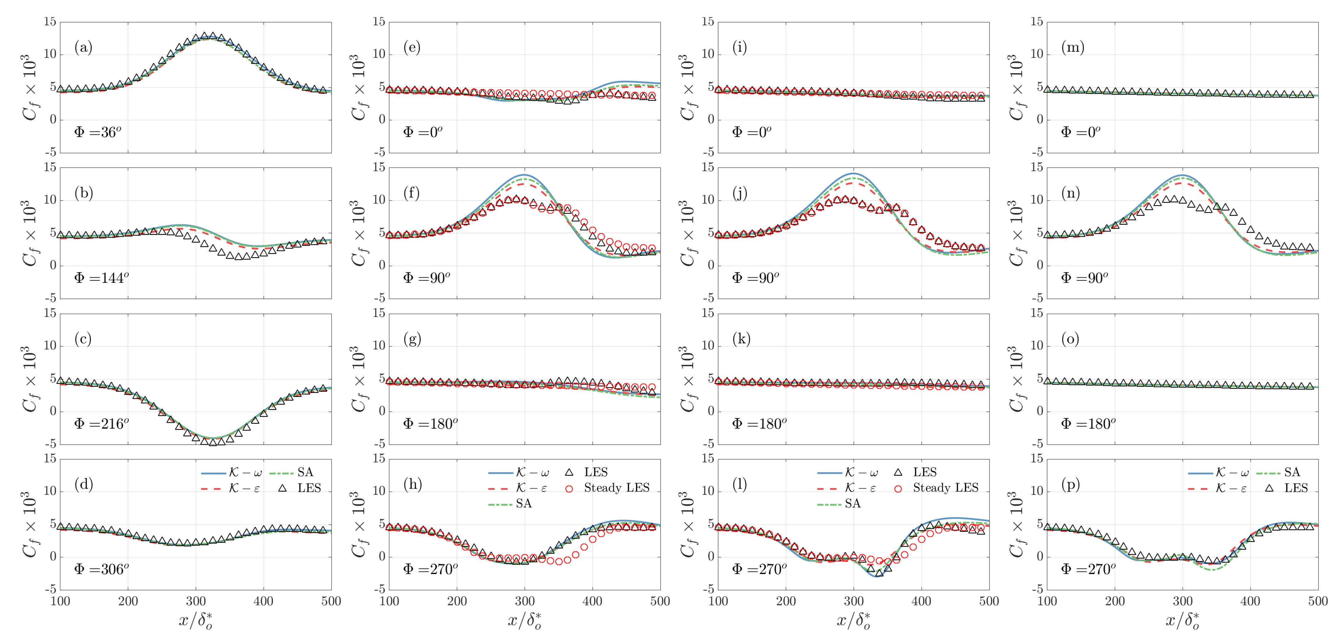
Figure 8.
Time evolution of (a–c) and (d–f) at the center of the recirculation region (). (a,d) ; (b,e) ; (c,f) .
Figure 8.
Time evolution of (a–c) and (d–f) at the center of the recirculation region (). (a,d) ; (b,e) ; (c,f) .

Figure 9.
Recirculation zone dimensions during the cycle. (a) ; (b) ; (c) .
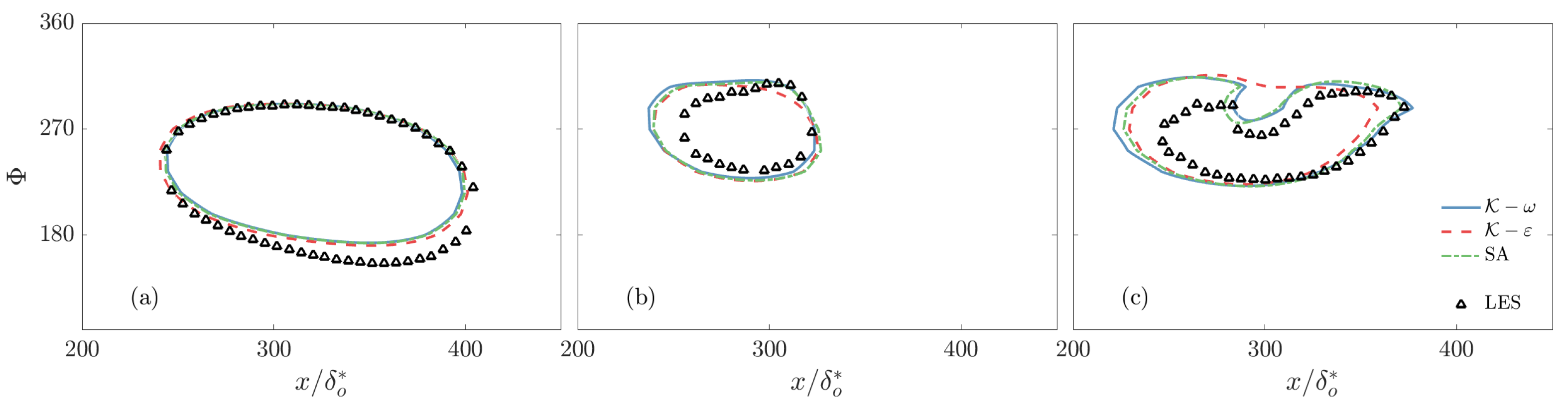
Figure 10.
Reynolds shear stress profiles () at three streamwise locations (, 300, and 400) and four phases, , and . (a–d) ; (e–h) ; (i–l) .
Figure 10.
Reynolds shear stress profiles () at three streamwise locations (, 300, and 400) and four phases, , and . (a–d) ; (e–h) ; (i–l) .
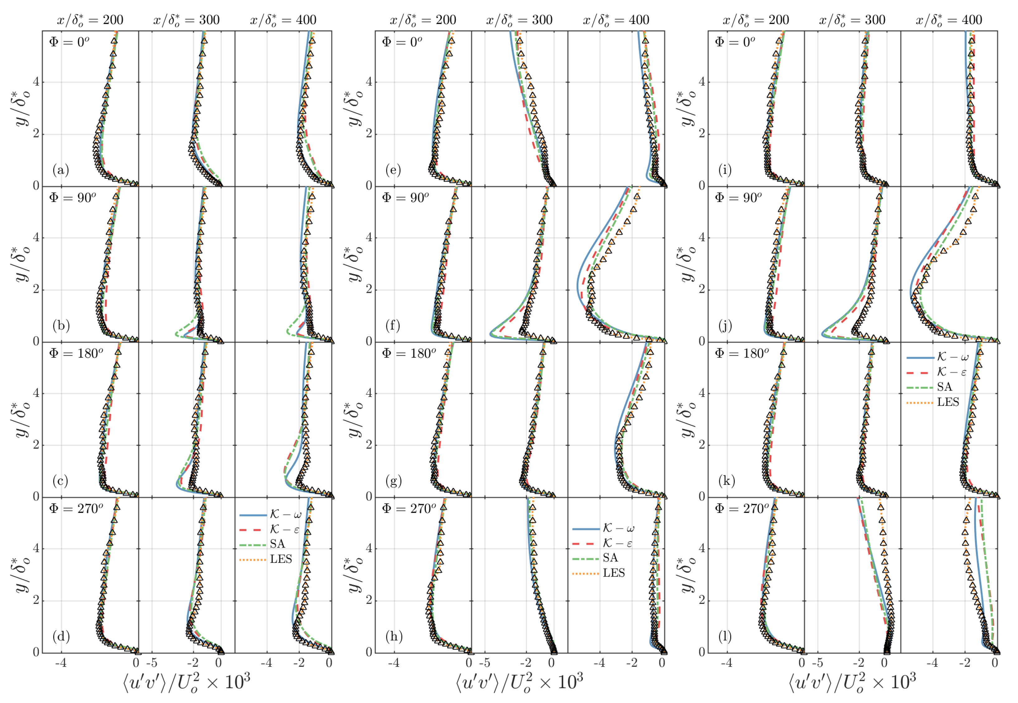
Figure 11.
(a–c) Normalized drag and (d–f) Integrated error. (a,d) ; (b,e) ; (c,f) .

Figure 12.
Case B. Contours of the phase-averaged streamwise velocity at (a–d) ; (e–h) . (a,e) – model; (b,f) – model; (c,g) SA model; (d,h) LES. The Supplementary Material contains an animation showing the entire cycle (Supplementary File S2).
Figure 12.
Case B. Contours of the phase-averaged streamwise velocity at (a–d) ; (e–h) . (a,e) – model; (b,f) – model; (c,g) SA model; (d,h) LES. The Supplementary Material contains an animation showing the entire cycle (Supplementary File S2).

Figure 13.
Case C. Contours of the phase-averaged streamwise velocity at (a–d) ; (e–h) . (a,e) – model; (b,f) – model; (c,g) SA model; (d,h) LES. The Supplementary Material contains an animation showing the entire cycle (Supplementary File S3).
Figure 13.
Case C. Contours of the phase-averaged streamwise velocity at (a–d) ; (e–h) . (a,e) – model; (b,f) – model; (c,g) SA model; (d,h) LES. The Supplementary Material contains an animation showing the entire cycle (Supplementary File S3).
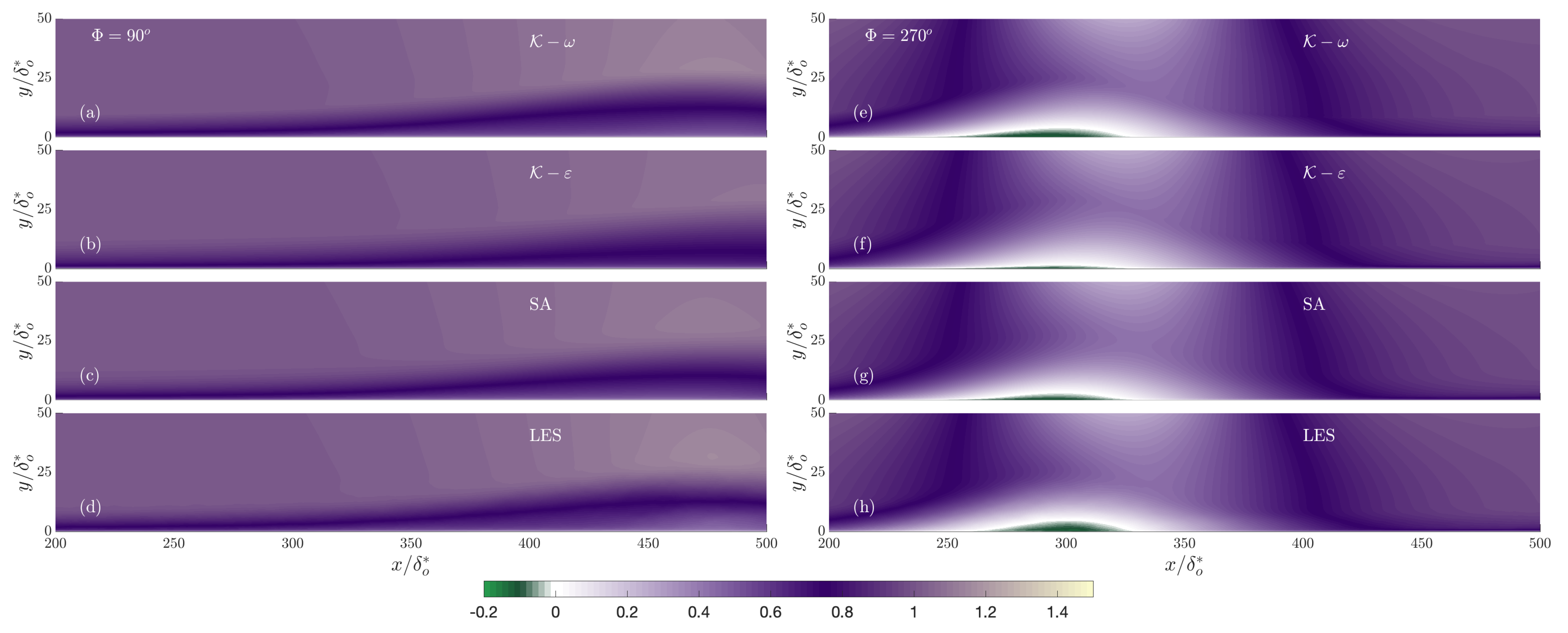
Figure 14.
Recirculation zone dimensions during the cycle. (a) Case A; (b) Case B; (c) Case C.

Figure 15.
Skin-friction coefficient at four phases in the cycle. (a–d) Case A; (e–h) Case B; (i–l) Case C.
Figure 15.
Skin-friction coefficient at four phases in the cycle. (a–d) Case A; (e–h) Case B; (i–l) Case C.

Figure 16.
Reynolds shear stress profiles at three streamwise locations (, 300, and 400) and four phases in the cycle. (a–d) Case A; (e–h) Case B; (i–l) Case C.
Figure 16.
Reynolds shear stress profiles at three streamwise locations (, 300, and 400) and four phases in the cycle. (a–d) Case A; (e–h) Case B; (i–l) Case C.
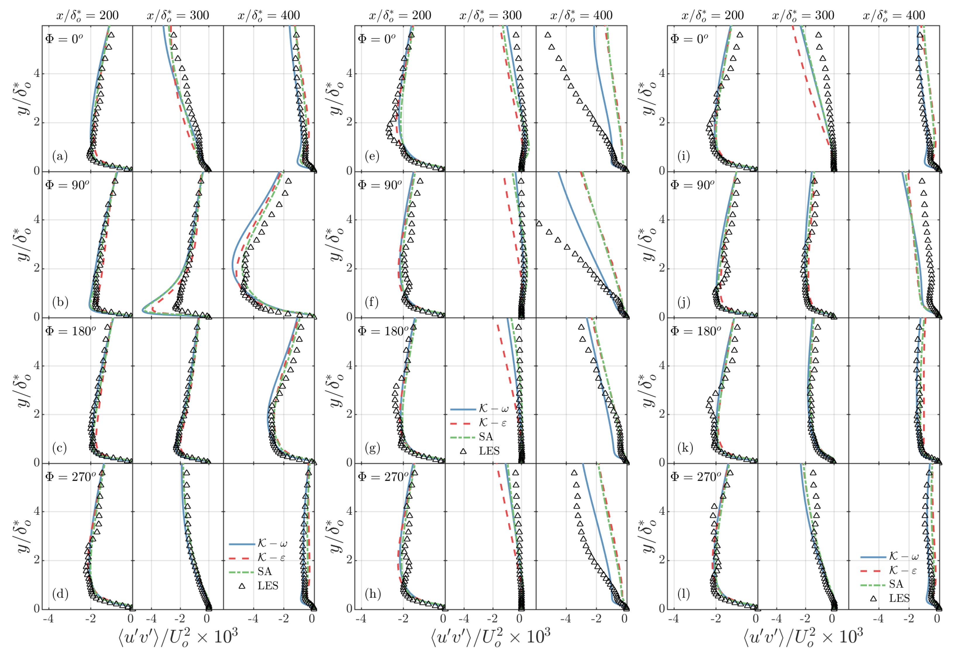
Figure 17.
Comparison of the skin-friction coefficient with the results of Park et al. [32]. (a) DNS, present LES and – model; (b) DNS, present LES and SA model.
Figure 17.
Comparison of the skin-friction coefficient with the results of Park et al. [32]. (a) DNS, present LES and – model; (b) DNS, present LES and SA model.
Disclaimer/Publisher’s Note: The statements, opinions and data contained in all publications are solely those of the individual author(s) and contributor(s) and not of MDPI and/or the editor(s). MDPI and/or the editor(s) disclaim responsibility for any injury to people or property resulting from any ideas, methods, instructions or products referred to in the content. |
© 2023 by the authors. Licensee MDPI, Basel, Switzerland. This article is an open access article distributed under the terms and conditions of the Creative Commons Attribution (CC BY) license (https://creativecommons.org/licenses/by/4.0/).
Share and Cite
MDPI and ACS Style
MacDougall, C.Y.; Piomelli, U.; Ambrogi, F. Evaluation of Turbulence Models in Unsteady Separation. Fluids 2023, 8, 273. https://doi.org/10.3390/fluids8100273
AMA Style
MacDougall CY, Piomelli U, Ambrogi F. Evaluation of Turbulence Models in Unsteady Separation. Fluids. 2023; 8(10):273. https://doi.org/10.3390/fluids8100273
Chicago/Turabian StyleMacDougall, Claire Yeo, Ugo Piomelli, and Francesco Ambrogi. 2023. "Evaluation of Turbulence Models in Unsteady Separation" Fluids 8, no. 10: 273. https://doi.org/10.3390/fluids8100273