Numerical Approach Based on Solving 3D Navier–Stokes Equations for Simulation of the Marine Propeller Flow Problems

Abstract

The report presents the approach implemented in the Russian LOGOS software package for the numerical simulation of the marine propeller flow problems using unstructured computational meshes automatically generated by the mesh generator. This approach includes a computational model based on the Navier–Stokes equation system and written with respect to the physical process: the turbulent nature of flow with transient points is accounted using the Reynolds Averaged Navier–Stokes method and the k–ω SST model of turbulence by Menter along with the γ–Re_θ (Gamma Re Theta) laminar-turbulent transition model; the Volume of Fluid method supplemented with the Schnerr–Sauer cavitation model is used to simulate the cavitation processes; a rotating propeller is simulated by a moving computational mesh and the GGI method to provide conformity of the solutions on adjacent boundaries of arbitrarily-shaped unstructured meshes of the two domains. The specific features of the numerical algorithms in use are described. The method validation results are given; they were obtained because of the problems of finding the performance curves of model-scale propellers in open water, namely the problems of finding the performance of propellers KP505 and IB without consideration of cavitation and the performance of propellers VP1304 and C5 under cavitation conditions. The paper demonstrates that the numerical simulation method presented allows for obtaining sufficiently accurate results to predict the main hydrodynamic characteristics for most modes of operation of the propellers.

1. Introduction

For many typical problems in shipbuilding, there is a need to simulate ship propulsors; one option is a marine propeller. Its performance is characterized by such quantities as thrust and torque. The dependences of these dimensionless parameters and the propeller efficiency on the advance ratio form the propeller performance curves. It is important to find these hydrodynamic parameters for the further integrated simulation of the self-propulsion tests.

One of the advanced approaches used to predict the propeller performance is a 3D numerical simulation with a description of the propeller geometry and that account for the specific physical processes: rotation of a body, the turbulent nature of flow with transient points, cavitation processes, the effect of closeness to the water surface, and waves. The basis of such an approach is a computational model based on the Navier–Stokes equation system written with respect to the abovementioned factors [1]. For example, to take into account the behavior of a turbulent flow, one can use the RANS (Reynolds Averaged Navier–Stokes) method [2,3,4] or the space filtering methods (the eddy-resolving approaches, such as the LES (Large Eddy Simulation) method, and hybrid methods) [5,6,7]. The RANS method is widely used for the numerical simulation of propellers and allows for achieving an acceptable accuracy of the solution [8,9,10,11,12]. The quality of RANS simulation results may depend on the chosen types of computational mesh and turbulence models (see [10,11]). It is shown in paper [12] that the use of the laminar-turbulent transition model in numerical simulations allows for improving the prediction accuracy for the hydrodynamic characteristics of propellers at the model scale. For details on the use of the eddy-resolving approaches to simulate the propeller flow problems, see [13,14,15,16,17]. They allow for improving the accuracy and reproducing a complex flow structure; however, with the use of such an approach, one faces difficulties in accounting for the laminar-turbulent transition.

The operation of a propeller may be accompanied by the cavitation processes, which often lead to the deterioration of the functional performance, the wear of the propeller component parts, and a lower efficiency [18]. The most popular way of taking into account cavitating flows is to use the VOF (Volume of Fluid) method [19,20] to describe the dynamics of phases and models of cavitation [21,22,23,24], which are the relation between the mass transfer velocity of the liquid and vapor phases and the flow parameters. Such an approach is used in [25,26,27,28,29,30] and provides a sufficiently accurate description of the shape of cavities and their dynamics.

The propeller flow problems are closely associated with the aspect of the numerical simulation of rotation. There are two approaches to consider a rotating body: implicit rotation, which is simulated by a moving frame of a reference algorithm [9,31], and explicit rotation, which is simulated using a computational mesh moving together with the propeller boundaries [10,25]. The advantage of the implicit rotation method is that it does not require consideration of the motion of the body boundaries in each time step; however, the method cannot be used for a steady structure (for example, the hull of a ship). For the simulation of a propeller and a hull, the explicit rotation method is used as a universal method.

The paper describes the propeller flow simulation method using unstructured computational meshes generated by the automatic mesh generator. Special consideration is given to the features of the implementation of numerical algorithms, the algorithm for taking into account rotation and determination the flow caused by the motion of the mesh in particular. The method is based on solving the system of Navier–Stokes equations averaged according to Reynolds, which is closed with the Menter’s k–ω SST model of turbulence [32] jointly with the γ–Re_θ (Gamma Re Theta) laminar-turbulent transition model [33]. The cavitation processes are accounted for using the VOF method supplemented with the SS (Schnerr–Sauer) model of cavitation [21]. A rotating propeller is simulated by moving nodes of the computational mesh with the interpolation of fluxes across a non-conformal mesh interface. The method is implemented in the LOGOS CAE system [27,34] for the simulation of coupled 3D problems of heat and mass transport with convection, aerodynamics, hydrodynamics, and strength analysis on computers with massive parallelism. Verification results are given for the problems of finding the performance curves of model-scale propellers operating in open water, with the cavitation process being taken or not taken into account.

2. Description of the Method for Numerical Simulation of the Propeller Flow Problems

2.1. Governing Equations and Turbulence Modeling

The flow around a propeller is a turbulent flow. Currently, the simulation of turbulent flows was performed using the RANS [35], LES [36], and hybrid methods [37,38]. In the RANS approach, the Navier–Stokes equations averaged according to Reynolds (averaging symbols were omitted) [39] were used to describe the turbulent motion of a viscous liquid/gas:

$$\{\begin{array}{l}\frac{\partial \rho }{\partial t}+\frac{\partial }{\partial x_i}\left(\rho u_i\right)=0,\\ \frac{\partial \rho u_i}{\partial t}+\frac{\partial }{\partial x_j}\left(\rho u_i{u}_j\right)=-\frac{\partial p}{\partial x_i}+\frac{\partial }{\partial x_j}\left({\tau }_{ij}+{\tau }^t{}_{ij}\right)+\rho g_i,\end{array}$$

(1)

where t was time; i, j were subscripts indicating the vector components in Cartesian coordinates, i, j = {x, y, z}; u_i was the velocity vector component; x_i was the Cartesian coordinate vector component; τ_ij was the viscous stress tensor; ${\tau }_{ij}^t$ was the Reynolds stress tensor; g_i was the gravitational acceleration vector component; p was pressure; ρ was density of liquid.

The rheological Newton law defines the viscous stress tensor components [35]:

$${\tau }_{ij}=\mu \left(\frac{\partial u_i}{\partial x_j}+\frac{\partial u_j}{\partial x_i}-\frac{2}{3}\frac{\partial u_k}{\partial x_k}{\delta }_{ij}\right),$$

(2)

where μ is dynamic viscosity and δ_ij is Kronecker symbol.

Linear differential models of turbulence use empirical relations to calculate the turbulent viscosity coefficient μ_t and the Boussinesq hypothesis for the Reynolds stress tensor calculation:

$${\tau }^t{}_{ij}=2{\mu }_t\left(S_{ij}-\frac{1}{3}\frac{\partial u_k}{\partial x_k}{\delta }_{ij}\right)+\frac{2}{3}k{\delta }_{ij}, S_{ij}=\frac{1}{2}\left(\frac{\partial u_i}{\partial x_j}+\frac{\partial u_j}{\partial x_i}\right),$$

(3)

where k is kinetic energy of turbulence.

The turbulence model closes the system of Equation (1). In the present paper, the k–ω SST model by Menter [32] and the γ–Re_θ laminar-turbulent transition model [33] were used.

2.2. Cavitating Flow Modeling

In case of a cavitating flow, a mathematical model is required, which takes into account the phase transition and the vapor medium motion. The VOF method [19], which can be easily generalized to the case of unstructured meshes and an arbitrary number of phases, is commonly used to simulate a multiphase medium. To describe the mass transfer processes (evaporation and condensation), the SS model of cavitation [21] was used; it is based on solving the Rayleigh–Plesset equation describing the dynamics of a single vapor bubble. With such an approach, Equation (1) was supplemented with the equation for the volume fraction transport of one of the phases, for example, vapor:

$$\{\begin{array}{l}\frac{\partial \rho }{\partial t}+\frac{\partial }{\partial x_i}\left(\rho u_i\right)=0,\\ \frac{\partial \rho u_i}{\partial t}+\frac{\partial }{\partial x_j}\left(\rho u_i{u}_j\right)=-\frac{\partial p}{\partial x_i}+\frac{\partial }{\partial x_j}\left({\tau }_{ij}+{\tau }^t{}_{ij}\right)+\rho g_i,\\ \frac{\partial {\rho }_v{\alpha }_v}{\partial t}+\frac{\partial }{\partial x_i}\left({\rho }_v{\alpha }_v{u}_i\right)=R_e-R_c,\end{array}$$

(4)

where ρ was the resultant density in the given case, which was the averaged density of the two phases: ρ = ρ_lα_l + ρ_vα_v, α was a volume fraction (subscript v was used for vapor, subscript l was used for liquid); R_e, R_c were the mass sources describing the generation and collapse of vapor bubbles.

To find the evaporation and condensation parameters—R_e and R_c—the SS model uses the ratio between the volume fraction of vapor and the number of bubbles per unit volume:

$${\alpha }_v=\frac{n\frac{4}{3}\pi r_B^3}{1+n\frac{4}{3}\pi r_B^3},$$

(5)

where n is the number of bubbles per unit volume and r_B is radius of a bubble.

It was assumed that the volume fraction of vapor varied in time only due to variations in the bubble radii, and hence, we calculated the following:

$$\frac{d{\alpha }_v}{dt}=-\frac{d}{dt}(1-{\alpha }_v)=\frac{n4\pi r_B^2}{{\left(1+n\frac{4}{3}\pi r_B^3\right)}^2}\frac{d{r}_B}{dt}=\frac{3}{r_B}{\alpha }_v(1-{\alpha }_v)\frac{d{r}_B}{dt}.$$

(6)

If pressure p in the liquid surrounding a given bubble was higher than pressure p_B of saturated vapors, the evaporation process took place with an increasing radius of bubbles r_B; otherwise, the condensation process with a decreasing radius of bubbles was observed. According to the Rayleigh–Plesset equation, the r_B growth rate could be written as follows:

$$\frac{d{r}_B}{dt}=\{\begin{array}{l}\sqrt{\frac{2}{3}(\frac{p_B-p}{{\rho }_l}}), p\le p_B\\ -\sqrt{\frac{2}{3}(\frac{p-p_B}{{\rho }_l}}),\hspace{0.17em}\hspace{0.17em}p>p_B\end{array}.$$

(7)

With regard to (6) and (7), we could write the transport equation for the volume fraction of vapor:

$$\frac{\partial {\alpha }_v}{\partial t}+u_i\frac{\partial {\alpha }_v}{\partial x_i}=\frac{\rho }{{\rho }_l{\rho }_v}(R_e-R_c).$$

(8)

Here, the following expressions were used for R_e and R_c:

$$R_e=\frac{{\rho }_v{\rho }_l}{\rho }{\alpha }_v(1-{\alpha }_v)\frac{3}{r_B}\sqrt{\frac{2}{3}(\frac{p_B-p}{{\rho }_l})}\hspace{0.17em},\hspace{0.17em}p<p_B,$$

(9)

$$R_c=\frac{{\rho }_v{\rho }_l}{\rho }{\alpha }_v(1-{\alpha }_v)\frac{3}{r_B}\sqrt{\frac{2}{3}(\frac{p-p_B}{{\rho }_l})}\hspace{0.17em},\hspace{0.17em}p>p_B,$$

(10)

where ρ_v and ρ_l were the vapor and liquid phase densities, respectively; they were taken as a constant.

For the discretization purposes, the transport Equation (8) in its non-divergent form was used for the vapor volume fraction, and this allowed for improving the solution stability and accuracy [20,40]. In so doing, the continuity equation of system (4) was written with respect to velocity divergence:

$$\frac{\partial u_i}{\partial x_i}=-\frac{1}{\rho }\frac{d\rho }{dt}=-\frac{{\rho }_v-{\rho }_l}{\rho }\frac{d\alpha }{dt}=-\frac{{\rho }_v-{\rho }_l}{\rho }\frac{\rho }{{\rho }_l{\rho }_v}(R_e-R_c)=\left(\frac{1}{{\rho }_v}-\frac{1}{{\rho }_l}\right)(R_e-R_c).$$

(11)

This allowed us to get rid of the derivative $\frac{d\rho }{dt}$, which took large values in areas of free surface, and thereby improved stability of the iterative procedure of finding the solution [41].

For discretization of the convective term in the volume fraction transport equation, “compressive” schemes have proven themselves to be effective, which allow one to avoid front blurring. One of the known “compressive” schemes is the High Resolution Interface Capturing (HRIC) scheme [42], which was used in this paper.

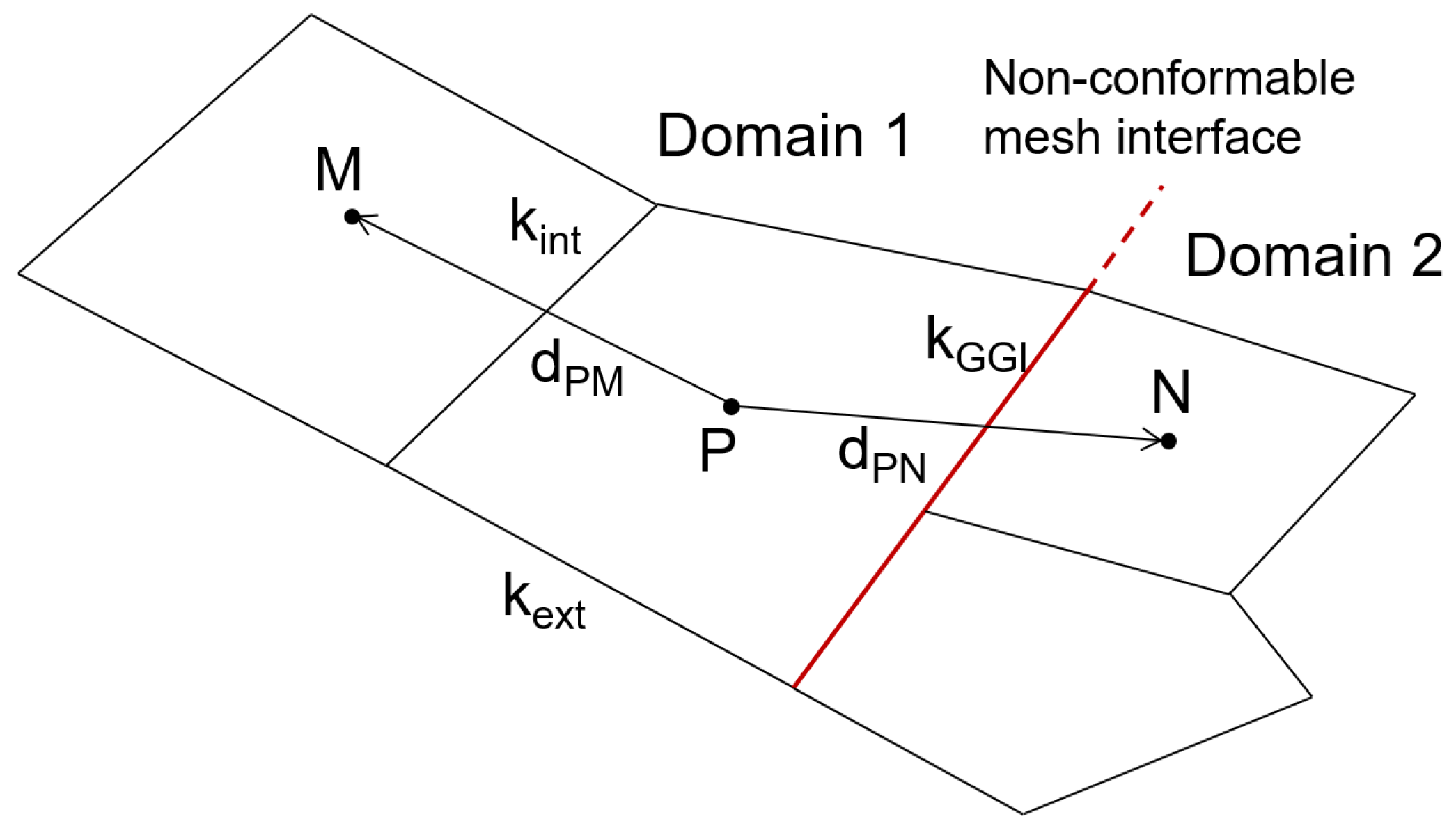
2.3. Rotation Modeling

A rotating body was simulated with the explicit method using a computational mesh moving together with the propeller boundaries. With such an approach, a domain near the propeller, in which the rotation took place, was selected, while the rest domain remained motionless (Figure 1).

In the rotation domain, the relation from [43] was used to take into account the mesh motion:

$$\frac{d^{*}\phi }{dt}=\frac{\mathrm{\partial }\phi }{\mathrm{\partial }t}+v_i\frac{\mathrm{\partial }\phi }{\mathrm{\partial }{x}_i},$$

(12)

where $\frac{d^{*}\phi }{dt}$ was substantial derivative of transferable scalar φ relative to a moving system of coordinates; v_i was the displacement velocity vector of the computational mesh. Consider an example of using the volume fraction transport Equation (8). By using Equation (12), we could rewrite Equation (8) in the following way (subscript v was omitted for volume fraction):

$$\frac{d^{*}\alpha }{dt}+\frac{\partial }{\partial x_i}\left(\alpha \left(u_i-v_i\right)\right)-\alpha \frac{\partial }{\partial x_i}\left(u_i-v_i\right)-Q=0,$$

(13)

where Q = $\frac{\rho }{{\rho }_l{\rho }_v}(R_e-R_c)$.

The GGI (General Grid Interface) method [44] was used to conform solutions on adjacent boundaries of arbitrary unstructured meshes of the two domains and based on conservative interpolation of fluxes across non-conformable mesh interface. This algorithm takes into account connections of cells on adjacent boundaries of regions without modifications to the original mesh using a generated set of virtual faces and creating additional terms in the system of linear algebraic equations (SLAE) in each computation step. Figure 2 shows an example of merging two domains.

Cell P had a set of faces k, including internal faces k_int, external faces k_ext, and adjacent faces k_GGI of the two domains, which formed a non-conformable mesh interface. Cell M and cell P belonged to one and the same domain (Domain 1), while cell N belonged to the neighboring domain (Domain 2); the distances from the center of cell P to the centers of cells M and N were d_PM and d_PN, respectively. Consider the equation discretization by the example of Equation (13); it was based on the method of finite volumes with respect to the unstructured nature of the computational mesh. The time discretization of Equation (13) was performed using one of the known schemes; here, we used the implicit Euler scheme [45]:

$$\frac{{\alpha }_P^j-{\alpha }_P^{j-1}}{\mathrm{\Delta }t}+{\left[\frac{\mathrm{\partial }}{\mathrm{\partial }{x}_i}\left(\alpha \left(u_i-v_i\right)\right)?\alpha \frac{\mathrm{\partial }}{\mathrm{\partial }{x}_i}\left(u_i-v_i\right)-Q\right]}^j=0,$$

(14)

where ${\alpha }_P^j$ was the volume fraction at the center of cell P in the current time step; ${\alpha }_P^{j-1}$ was the volume fraction at the center of cell P in the previous time step.

For the space discretization of Equation (13), we integrated this equation over volume V_P of cell P. For the convective term, according to Ostrogradsky–Gauss theorem, we went to the integral over surface S_P (time indexes were omitted if they were evident):

$${\displaystyle \underset{V_P}{\int }\frac{{\alpha }_P^j-{\alpha }_P^{j-1}}{\Delta t}d{V}_P}+{\displaystyle \underset{S_P}{\int }\hspace{0.17em}\alpha \left(u_i-v_i\right)}d{S}_P-{\alpha }_P{\displaystyle \underset{S_P}{\int }\left(u_i-v_i\right)d{S}_P}-{\displaystyle \underset{V_P}{\int }Qd{V}_P}=0.$$

(15)

For approximation on a finite-volume mesh, we wrote the convective term of the form:

$$\begin{array}{c}{\displaystyle \underset{S_P}{\int }\alpha \left(u_i-v_i\right)} d{S}_P-{\alpha }_P{\displaystyle \underset{S_P}{\int }\left(u_i-v_i\right)d{S}_P}\approx {\displaystyle {\displaystyle \sum }_k}{\alpha }_k\left(u_{i,k}-v_{i,k}\right)S_{i,k}-{\alpha }_P{\displaystyle {\displaystyle \sum }_k}\left(u_{i,k}-v_{i,k}\right)S_{i,k}\approx \\ \approx {\displaystyle {\displaystyle \sum }_k}{\alpha }_k\left(F_k-F_k^v\right)-{\alpha }_P{\displaystyle {\displaystyle \sum }_k}\left(F_k-F_k^v\right),\end{array}$$

(16)

where k was the number of face; S_i,k was the area vector of face k; α_k was the volume fraction on face k; F_k was the volume flux across face k, which could be found by solving the continuity and momentum conservation equations; $F_k^v$ was the volume flux associated with the mesh motion; summation over all faces of cell P was performed. The quantity value on face α_k was determined by the discretization scheme [46].

To find the flux $F_k^v$, one can use the instant translational velocity of flux at the face center:

$${\overrightarrow{v}}_k=\overrightarrow{\omega }\times \overrightarrow{r},$$

(17)

where $\overrightarrow{\omega }$ is the angular velocity vector; $\overrightarrow{r}$ is radius-vector to a given point from the coordinate origin located on the body axis of revolution. However, with an increasing $\overrightarrow{r}$ the calculation error increases, and this leads to disbalance of fluxes $F_k^v$ and, as a result, to the perturbed numerical solution.

Alternatively, the flux $F_k^v$ can be found exactly in the calculation of the volume created by sweeping with a rotating face. Figure 3 shows the face k with vertices 1-2-3-4 and the volume V_k created by rotating this face about axis ω.

The flux $F_k^v$ can be found by sequentially summarizing the volumes of the bodies bounded by the surfaces of revolution of the face edges:

$$F_k^v=\frac{\omega }{2\pi }{\displaystyle \sum _{n=1}^N{V}_{n\to n+1}},$$

(18)

where n is a serial number of a vertex; N is the total number of edges.

For this purpose, we found the cylindrical coordinates of the vertices of each edge. The z coordinate of vertex 1 was as follows:

$$z_1={\overrightarrow{d}}_1·{\overrightarrow{n}}_{\omega },$$

(19)

where ${\overrightarrow{d}}_1$ was radius-vector from the center of revolution to vertex 1; ${\overrightarrow{n}}_{\omega }$ was a unit vector of the ω axis of revolution.

The r coordinate of vertex 1 was as follows:

$$r_1=\left|{\overrightarrow{r}}_1\right|=\left|{\overrightarrow{d}}_1-z_1·{\overrightarrow{n}}_{\omega }\right|,$$

(20)

where ${\overrightarrow{r}}_1$ was a vector normal to z axis.

Similarly, one can find the z₂ and r₂ coordinates of vertex 2. The volume formed by rotating the edge 1–2 can be calculated via the following integral:

$$V_{1-2}={\displaystyle \underset{z_1}{\overset{z_2}{\int }}\pi r^2}(z)dz,$$

(21)

where $r(z)=r_1+\frac{r_2-r_1}{z_2-z_1}(z-z_1)$.

One can integrate (21) and take $\frac{r_2-r_1}{z_2-z_1}=b$ to obtain the following:

$$V_{1-2}=\pi (z_2-z_1)\left(r_1^2+r_{1}b(z_2-z_1)+\frac{1}{3}{b}^2{(z_2-z_1)}^2\right).$$

(22)

One can use expression (22) to find the volume created by sweeping for each edge of the face k and then find $F_k^v$ from (18).

2.4. Solution Algorithm

For the numerical solution of the system of Equation (4), SLAEs were generated according to the SIMPLE algorithm [1,35,47,48], in which the velocity and pressure fields could be found using the predictor–corrector scheme.

To formulate the SIMPLE algorithm, we wrote the equation of conservation of the momentum of the system (4) with time discretization from the Euler scheme (for brevity, we omitted the expansion of the stress tensor and the gravitational term):

$$\frac{{\rho }^n{u}_i^{n+1}-{\rho }^j{u}_i^j}{\Delta t}+\frac{\partial }{\partial x_j}\left({\rho }^n{u}_i^{n+1}{u}_j^n\right)=-\frac{\partial p^{n+1}}{\partial x_i}+\frac{\partial }{\partial x_j}\left({\tau }_{ij}^{n+1}\right).$$

(23)

Here, n was the solution at the previous iteration, and j was the solution at the previous time step. To solve this equation, the pressure and the velocity were presented in the following form:

$$\begin{array}{l}{u}_i^{n+1}=u_i^n+u_i^{*},\\ \\ p^{n+1}=p^n+{\alpha }_p(p^{n+1}-p^n)=p^n+{\alpha }_p\delta p^{n+1},\end{array}$$

(24)

where $0\le {\alpha }_p\le 1$ was a relaxation parameter. Substitution of the above expression into (23) yielded the following:

$$\frac{{\rho }^n{u}_i^{n+1}-{\rho }^j{u}_i^j}{\Delta t}+\frac{\partial }{\partial x_j}\left({\rho }^n{u}_i^{n+1}{u}_j^n\right)=-\frac{\partial p^n}{\partial x_i}-\frac{\partial \left(\delta p^{n+1}\right)}{\partial x_i}+\frac{\partial }{\partial x_j}\left({\tau }_{ij}^{n+1}\right).$$

(25)

Substitution of the first expression in (24) into (23) allowed for obtaining a preliminary estimate of the velocity at the next step from the equation:

$$\frac{{\rho }^n{u}_i^{*}}{\Delta t}+\frac{\partial }{\partial x_j}\left({\rho }^n{u}_i^{*}{u}_j^n\right)-\frac{\partial }{\partial x_j}\left({\tau }_{ij}^{*}\right)=\frac{{\rho }^j{u}_i^j}{\Delta t}-\frac{\partial p^n}{\partial x_i}.$$

(26)

The molecular and turbulent components of the shear stress tensor in (26) were calculated using $u_i^{*}$ as well. At the second stage, the total speed was calculated at iteration n + 1 using a pressure correction:

$$u_i^{n+1}=u_i^{*}-\Delta t\frac{\partial \left(\delta p^{n+1}\right)}{\partial x_i}.$$

(27)

The pressure correction itself was found from Equation (27) if the continuity condition for $u_i^{n+1}$ was satisfied. Thus, taking the derivative of both sides of the above equality, we obtained the following Poisson equation for the pressure:

$$\frac{\partial }{\partial x_i}\left(\frac{\partial \left(\delta p^{n+1}\right)}{\partial x_i}\right)=\frac{1}{\Delta t}\frac{\partial u_i^{*}}{\partial x_i}.$$

(28)

This iterative procedure allowed for obtaining velocity and pressure fields that satisfy the system of Equation (4). To ensure the stability of the calculation, the right side of the continuity Equation (11) was linearized with respect to the pressure increment.

To take into account the force of gravity, we used the algorithm based on the correction of volume forces [20,49], which provided no oscillations induced by disposition of unknown quantities at the centers of cells. The multigrid method [50] allowed for accelerating computations on high-performance supercomputers.

The numerical simulation method described above was implemented in the LOGOS software package [27,34].

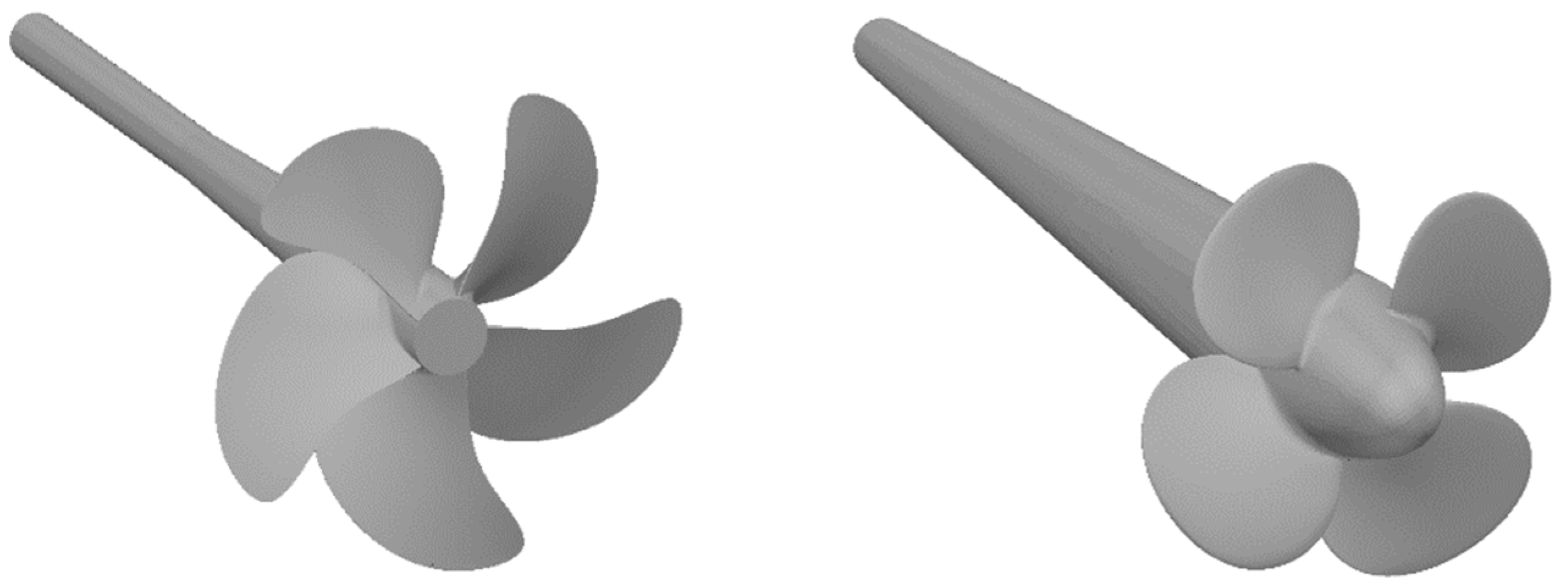
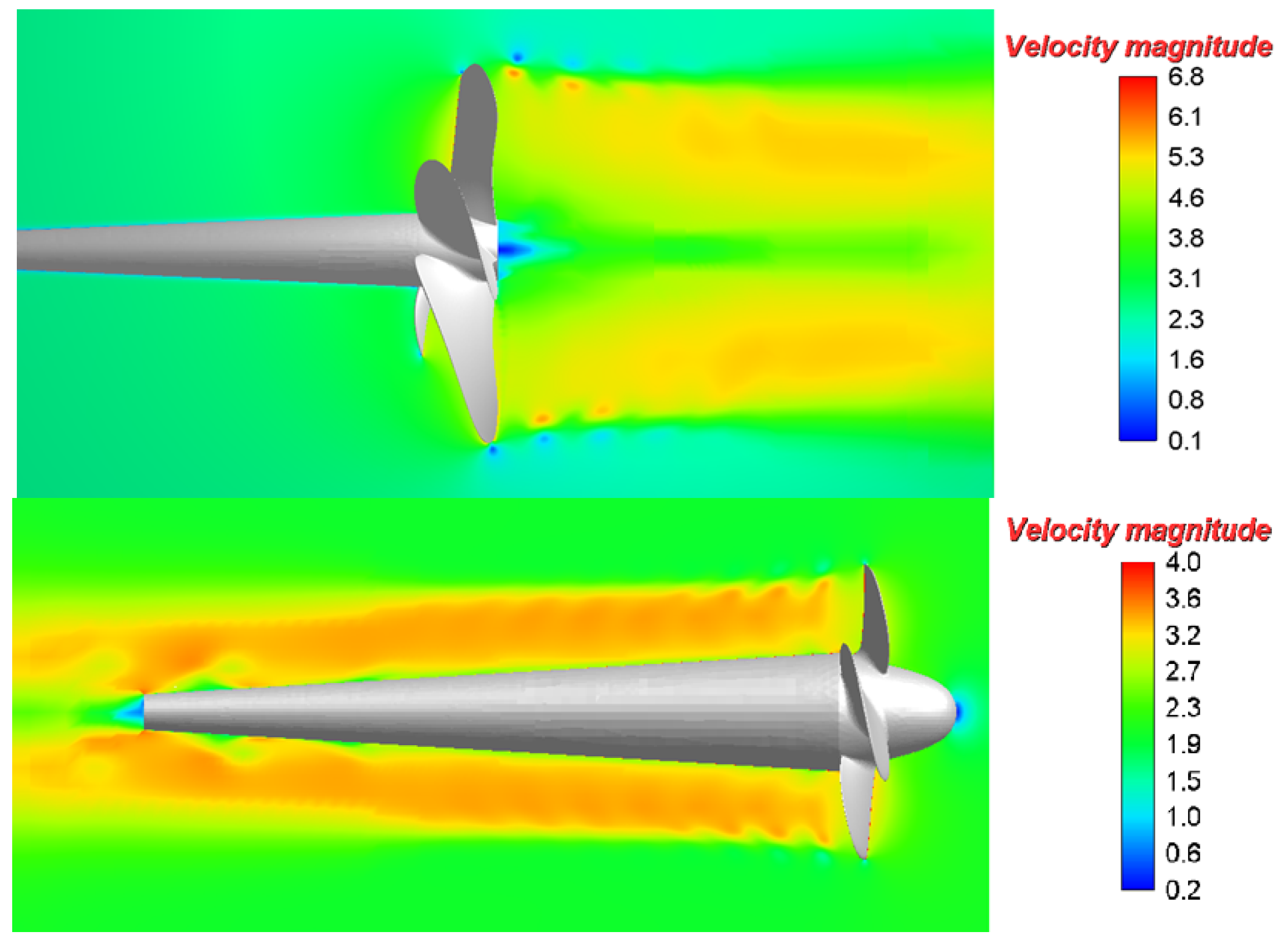
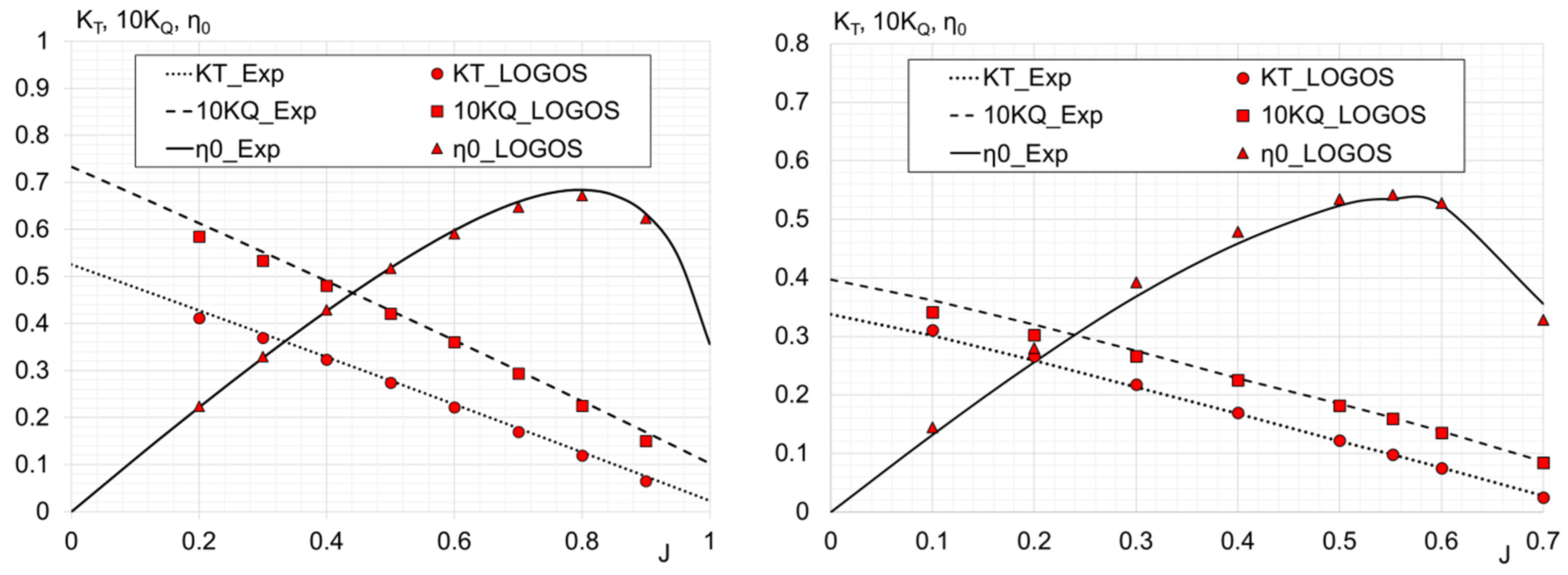
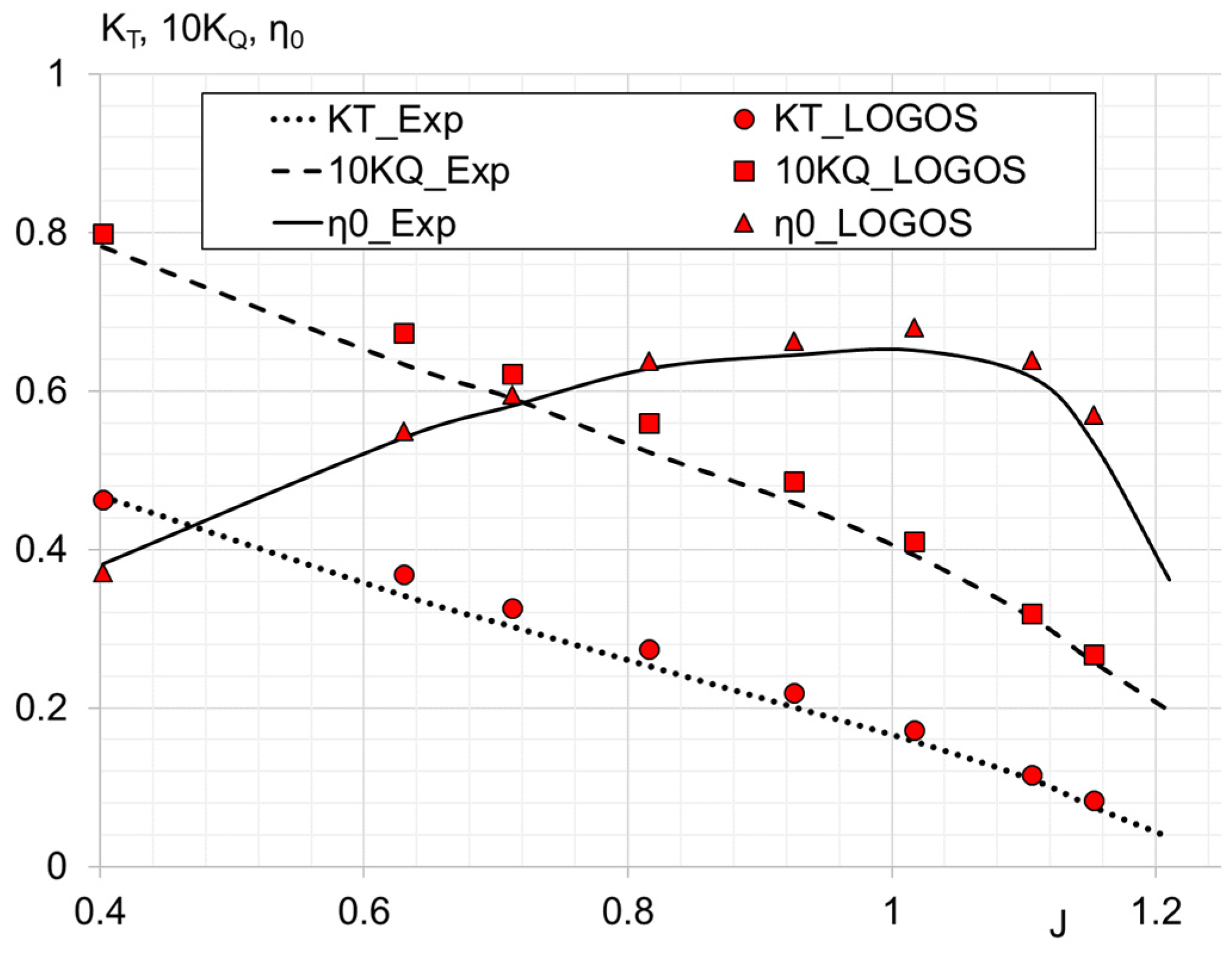
3. Numerical Calculation of the Propeller Performance in Open Water

First, the method is verified on the problems of a homogeneous liquid flow around propellers KP505 and IB without consideration of cavitation. The propellers are fixed at the shaft end, the KP505 model diameter is 0.25 m, and the IB model diameter is 0.2 m. Figure 4 shows the geometry of these propellers.

The performance curves of these propellers are calculated in a series of computations with the speed of rotation n = 20 rps. The advance ratio J in these computations varies in the range 0.1 ÷ 0.9 with increment 0.1; the incoming flow velocity is calculated with the following formula:

V = J · n · D,

(29)

where D is the propeller diameter. The range of values of the incoming flow velocity is 1 ÷ 4.5 m/s for propeller KP505 and 0.4 ÷ 2.8 m/s for propeller IB.

The computational meshes in Figure 5 were generated with a higher concentration of cells near blades, in the swirling flow motion direction, and in the boundary layer. The KP505 model mesh contains 15 mln cells, and the IB model mesh contains 5.8 mln cells. The computational meshes consist of two regions: the rotating internal region and the stationary external one. Both regions are cylinders; the propeller fixed at the shaft end is inside the rotating region.

The incoming flow velocity is set on the inlet boundary, pressure is set on the outlet boundary, the propeller boundaries are non-slip walls, and the lateral boundary of the computational domain is a slip wall.

The following physical properties of water were taken for computations: dynamic viscosity µ_l = 0.00114 Pa∙s and density ρ_l = 1000 kg/m³.

Figure 6 illustrates the instantaneous velocity field at time t = 1 s (J = 0.4 for KP505, J = 0.5 for IB).

One can see from Figure 6 the swirling flow and the velocity magnitude distribution near the propeller.

A quantitative comparison between the numerical simulation results is made for the propeller characteristics, such as the thrust coefficient K_T, the torque coefficient K_Q, and the efficiency η₀, which are calculated using the following formulas:

$$K_T=\frac{T}{\rho ·n^2·D^5}, K_Q=\frac{Q}{\rho ·n^2·D^5}, {\eta }_0=\frac{J}{2\pi }·\frac{K_T}{K_Q},$$

(30)

where T is thrust and Q is torque.

Figure 7 shows the action curves for KP505 and IB propellers obtained using the LOGOS software package in comparison with experimental data [51,52].

As one can see from Figure 7, the numerical simulation results are in good agreement with the experimental data. Errors in the predicted torque coefficient and thrust coefficient values achieve their maximum for the advance ratios close to 1 because of the small values of the above quantities in such modes of the propeller behavior. As a result, the efficiency calculation error also increases. Discrepancies in the resultant values of the propeller characteristic are below 5% for the advance ratio J below 0.5. A maximum discrepancy in the efficiency calculation results for propeller IB is observed for J = 0.7 (near the point of zero thrust) and equals 7.9%. A maximum deviation in the efficiency value for propeller KP505 is observed for J = 0.8 and equals 1.8%.

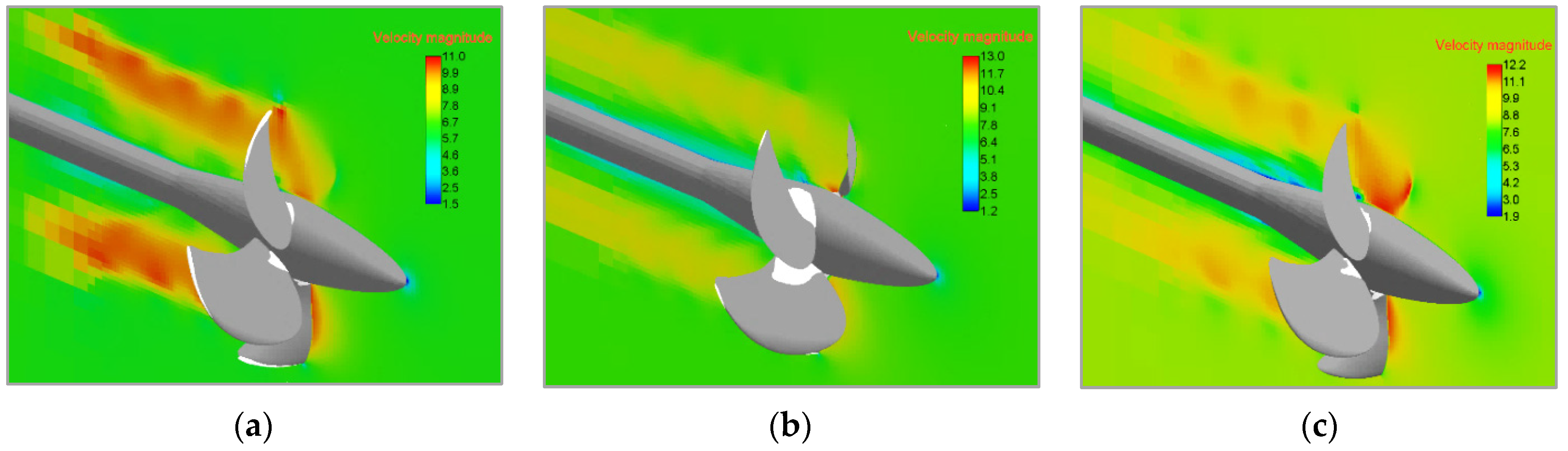
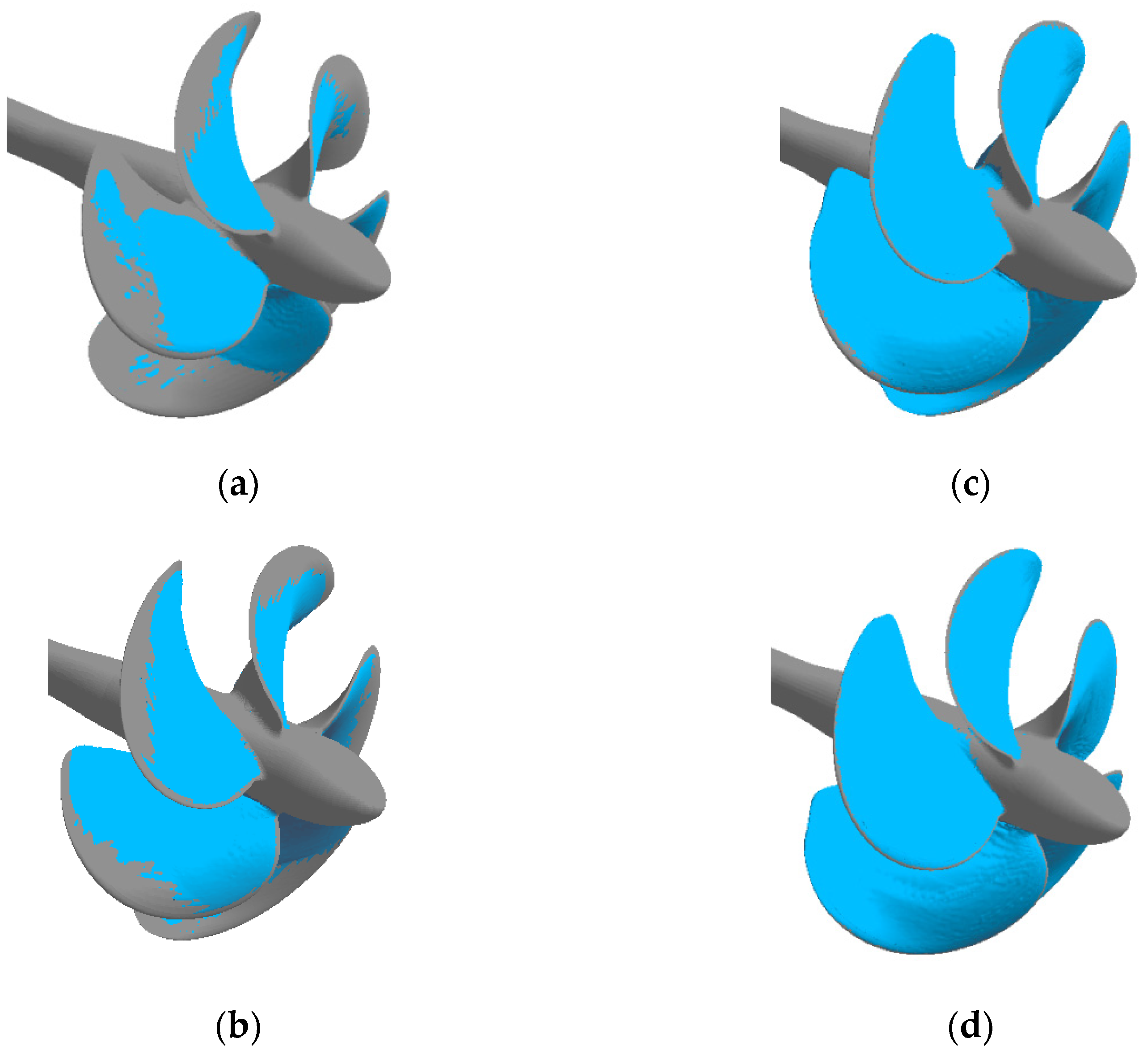
4. Numerical Calculation of the Propeller Performance under Cavitation Conditions

The validation of the methods used to simulate the performance of propellers with cavitation considered is performed on the problem of a liquid flow around a model of a rotating five-blade VP1304 propeller.

For flows with cavitation effects, the governing parameter is the cavitation number, σ. In the problems of a flow around a propeller, the cavitation number is as follows:

$$\sigma =\frac{(P-P_{sat})}{\rho n^2{D}^2/2}$$

(31)

where P is pressure and P_sat is saturation pressure.

Table 1. Computation modes.

Mode	1	2	3
Pressure in tube, Pa	43,071	31,353	42,603
Advance ratio	1.09	1.269	1.408
Cavitation number	2.024	1.424	2.0

gives experimental parameters for cavitating flows around the VP1304 propeller. The saturated vapor pressure calculated using the water temperature is P_sat = 3540 Pa.

In the experiments, the propeller thrust and torque were measured and used to calculate dimensionless hydrodynamic parameters using Formula (30).

The VP1304 propeller model, which geometry is shown in Figure 8, is fixed at the shaft end; the propeller diameter equals 0.25 m.

The computational mesh was built using the cutoff method with the mesh refinement near blades, in the swirling flow motion direction, and in the boundary layer. Figure 9 shows the VP1304 propeller model near its blade. The total number of the computational mesh cells is 2.8 mln.

The incoming flow velocity is set on the inlet boundary, the boundary condition with a fixed hydrostatic pressure distribution is set on the outlet boundary, the lateral boundary is a slip wall, and the propeller boundaries are non-slip walls.

To calculate the performance curves of the propeller, a series of computations was carried out with the speed of rotation n = 25 rps. The advance ratio J varied within the range of 1.09 ÷ 2.0; the advance ratios were used to calculate the incoming flow velocity with Formula (29).

The following physical parameters were taken for computations: dynamic viscosity µ_l = 0.00114 Pa∙s and density ρ_l = 1000 kg/m³ for water and dynamic viscosity µ_v = 1.26765∙10⁻⁵ Pa∙s and density ρ_v = 0.59531 kg/m³ for vapor.

Figure 10 shows the fields of velocity magnitude in the cross-section for the three flow conditions.

Figure 11 illustrates the shapes of cavitating regions for each calculated flow condition in comparison with experimental sketches.

One can see from these figures that in all cases, the shapes of cavitation clouds agree with experimental sketches. Similarly to the experiment, for the first two types of conditions (modes 1 and 2), the computation predicts the generation of two cavitating regions: one near the blade base and another along the front edge of the blade. For the second type of conditions (mode 2), where the cavitation number is smaller, the cavitation cloud is pronounced, both in the experiment and in the numerical simulation results. For the third type of conditions (mode 3), the comparison with the experimental sketch of cavitation vapor on the pressure side of the blade shows that the calculated fields are slightly different, and there is no detached flow at the end of the blade.

Figure 12 shows, in comparison, the performance curves of VP1304 propeller obtained using LOGOS and experimental data [53].

For mode 1, the difference in the values of coefficients K_T and K_Q does not exceed 1.8%. For mode 2, the maximum deviation is observed for the torque coefficient and equals 5.6%. For mode 3, the maximum deviation is 5.2% for K_Q and 4.4% for K_T. The calculated thrust coefficients for the advance ratios close to 1 are almost the same as in the experiments, while for higher advance ratios, they take values less than the experimental ones. The maximum deviation in the efficiency value is observed for mode 2 and equals 1.2%.

The next considered is the problem of a flow around a rotating model of five-blade C5 propeller. The model is fixed at the shaft end; the propeller diameter is 0.2 m. Figure 13 shows the model geometry.

To calculate the performance curves of the propeller, a series of computations was carried out for the cavitation numbers σ = 0.9 and σ = 1.2. The propeller rotation speed n varies within the range of 30 ÷ 36 rps, the incoming flow velocity is 5.5 m/s for σ = 0.9 and 5.2 m/s for σ = 1.2, and the advance ratio J is calculated with Formula (29).

The computational mesh in Figure 14 is built with the refinement of cells near blades, in the swirling flow motion direction, and in the boundary layer. The mesh model contains 10.2 mln cells.

The incoming flow velocity is set on the inlet boundary, the boundary condition with a fixed hydrostatic pressure distribution is set on the outlet boundary, the lateral boundary is a slip wall, and the propeller boundaries are non-slip walls.

The physical properties of water and vapor are the same as in the previous problem; the saturated vapor pressure is P_sat = 2325 Pa.

First, non-cavitating flows around the propeller are calculated. Figure 15 shows the performance curves of the C5 propeller model calculated using LOGOS in comparison with the experiment [54].

An error in the thrust coefficient prediction takes its maximum values with high advance ratios, and as a result, the efficiency calculation error increases. The maximum discrepancy in the calculated efficiency is 4.5% for the advance ratio J = 1.017.

Then, computations are carried out for the cavitation flow conditions. Figure 16 shows the velocity magnitude distribution in the central section of the computational domain for different rotation speeds of the propeller and different cavitation numbers.

Figure 17 shows the isosurface position of the volume fraction of the cavitation vapor obtained using LOGOS for different propeller rotation speeds and different cavitation numbers.

One can see the distribution of velocity magnitudes near the propeller and the cavitation cloud distribution.

Figure 18 shows the performance curves for the C5 propeller under cavitation conditions calculated using LOGOS in comparison with experimental data [47] for the cavitation numbers σ = 0.9 and σ = 1.2 (black solid lines—experimental performance curves for C5 propeller without consideration of cavitation).

The numerical simulation results obtained with LOGOS are in a good agreement with the reference data. Maximum deviations are observed for σ = 1.2 at the highest rotation speed of the propeller: 8.8% for the thrust coefficient, 10.7% for the torque coefficient, and 4.1% for the efficiency. Under the rest conditions, deviations in the calculated characteristics do not exceed 5% and equal 2.5% on average.

5. Conclusions

The paper presents the methods implemented in the Russian LOGOS software package for the numerical simulation of marine propellers on the base of solving the system of Navier–Stokes equations averaged according to Reynolds and closed by the k–ω SST model of turbulence along with the γ–Re_θ laminar-turbulent transition model. The VOF method and the SS cavitation model are used to take into account the cavitation processes. The rotation of propellers is simulated by moving computational mesh nodes and the GGI method used to provide conformable solutions on adjacent boundaries of arbitrary unstructured meshes of two domains. The basic equations and approaches used in the LOGOS software package to solve these equations are described.

The method validation results are given for the problems of finding the performance curves of models of IB and KP505 propellers with cavitation not taken into account and for models of VP1304 and C5 propellers under cavitation conditions. The numerical simulation results demonstrate that these methods provide sufficiently accurate results (with deviations not exceeding 5%) in predicting the main hydrodynamic characteristics of propellers under most operating conditions.

References

1. Ferziger, J.H.; Peric, M. Computational Method for Fluid Dynamics; Springer: New York, NY, USA, 2002. [Google Scholar]
2. Spalart, P.R. Strategies for turbulence modelling and simulations. Int. J. Heat Fluid Flow. 2000, 21, 252–263. [Google Scholar] [CrossRef]
3. Corson, D.; Jaiman, R.; Shakib, F. Industrial application of RANS modelling: Capabilities and needs. Int. J. Comput. Fluid Dyn. 2009, 23, 337–347. [Google Scholar] [CrossRef]
4. Yusof, S.; Asako, Y.; Sidik, N.; Mohamed, S.; Japar, W. A Short Review on RANS Turbulence Models. CFD Lett. 2020, 11, 83–96. [Google Scholar]
5. Launder, B.E.; Spalding, D.B. Lectures in Mathematical Models of Turbulence; Academic Press: London, UK, 1972. [Google Scholar]
6. Sagaut, P. Large Eddy Simulation for Incompressible Flows: An Introduction; Springer: Berlin/Heidelberg, Germany, 2006. [Google Scholar]
7. Zhiyin, Y. Large-eddy simulation: Past, present and the future. Chin. J. Aeronaut. 2015, 28, 11–24. [Google Scholar] [CrossRef]
8. Da-Qing, L. Validation of RANS predictions of open water performance of a highly skewed propeller with experiments. J. Hydrodyn. 2006, 18, 520–528. [Google Scholar]
9. Guo, C.Y.; Zhao, D.G.; Sun, Y. Numerical simulation and experimental research on hydrodynamic performance of propeller with varying shaft depths. China Ocean Eng. 2014, 28, 271–282. [Google Scholar] [CrossRef]
10. Morgut, M.; Nobile, E. Influence of grid type and turbulence model on the numerical prediction of the flow around marine propellers working in uniform inflow. Ocean Eng. 2012, 42, 26–34. [Google Scholar] [CrossRef]
11. Bennaya, M.; Gong, J.; Hegaze, M.; Zhang, W. Numerical simulation of marine propeller hydrodynamic performance in uniform inflow with different turbulence models. Appl. Mech. Mater. 2013, 389, 1019–1025. [Google Scholar] [CrossRef]
12. Baltazar, J.; Rijpkema, D.; de Campos, J.F. On the use of the Γ−ReΘt transition model for the prediction of the propellerperformance at model-scale. Ocean Eng. 2018, 170, 6–19. [Google Scholar] [CrossRef]
13. Ahmed, S.; Croaker, P.; Doolan, C. Instability identification within ship propeller wakes. In Proceedings of the Sixth International Symposium on Marine Propulsors—SMP’19, Rome, Italy, 26–30 May 2019. [Google Scholar]
14. Asnaghi, A.; Feymark, A.; Bensow, R.E. Computational Analysis of Cavitating Marine Propeller Performance using OpenFOAM. In Proceedings of the Fourth International Symposium on Marine Propulsors—SMP’15, Austin, TX, USA, 4 June 2015. [Google Scholar]
15. Martin, V.; Krishnan, M. Large eddy simulation of crashback in marine propellers. In Proceedings of the 44th AIAA Aerospace Sciences Meeting and Exhibit, Reno, NV, USA, 9–12 January 2006. [Google Scholar]
16. Kumar, P.; Mahesh, K. Large eddy simulation of propeller wake instabilities. J. Fluid Mech. 2017, 814, 361–396. [Google Scholar] [CrossRef]
17. Posa, A.; Broglia, R.; Felli, M.; Cianferra, M.; Armenio, V. Hydroacoustic analysis of a marine propeller using large-eddy simulation and acoustic analogy. J. Fluid Mech. 2022, 947, A46. [Google Scholar] [CrossRef]
18. Franc, J.P.; Michel, J.M. Fundamentals of Cavitation. In Fluid Mechanics and Its Applications; Springer: Berlin/Heidelberg, Germany, 2004. [Google Scholar]
19. Hirt, C.W.; Nichols, B.D. Volume of fluid (VOF) method for the dynamics of free boundaries. J. Comput. Phys. 1981, 39, 201–225. [Google Scholar] [CrossRef]
20. Efremov, V.R.; Kozelkov, A.S.; Kornev, A.V.; Kurkin, A.A.; Kurulin, V.V.; Strelets, D.Y.; Tarasova, N.V. Method for taking into account gravity in free-surface flow simulation. Comput. Math. Math. Phys. 2017, 57, 1720–1733. [Google Scholar] [CrossRef]
21. Schnerr, G.H.; Sauer, J. Physical and numerical modeling of unsteady cavitation dynamics. In Proceedings of the Fourth International Conference on Multiphase Flow, New Orleans, LA, USA, 27 May–1 June 2001. [Google Scholar]
22. Zwart, P.J.; Gerber, A.G.; Belamri, T. A Two-phase flow model for predicting cavitation dynamics. In Proceedings of the Fifth International Conference on Multiphase Flow, Yokohama, Japan, 30 May–3 June 2004. [Google Scholar]
23. Kunz, R.F.; Boger, D.A.; Stinebring, D.R. A preconditioned Navier-Stokes method for two-phase flows with application to cavitation prediction. Comput. Fluids 2000, 29, 849–875. [Google Scholar] [CrossRef]
24. Singhal, K.; Athavale, M.M.; Li, H.; Jiang, Y. Mathematical Basis and Validation of the Full Cavitation Model. J. Fluids Eng. 2002, 124, 617–624. [Google Scholar] [CrossRef]
25. Ji, B.; Luo, X.; Peng, X.; Wu, Y.; Xu, H. Numerical analysis of cavitation evolution and excited pressure fluctuation around a propeller in non-uniform wake. Int. J. Multiph. Flow 2012, 43, 13–21. [Google Scholar] [CrossRef]
26. Paik, K.J.; Park, H.; Seo, J. URANS Simulations of Cavitation and Hull Pressure Fluctuation for Marine Propeller with Hull Interaction. In Proceedings of the Third International Symposium on Marine Propulsors—SMP’13, Launceston, Australia, 5–8 May 2013. [Google Scholar]
27. Kozelkov, A.; Kurkin, A.; Kurulin, V.; Plygunova, K.; Krutyakova, O. Validation of the LOGOS Software Package Methods for the Numerical Simulation of Cavitational Flows. Fluids 2023, 8, 104. [Google Scholar] [CrossRef]
28. Roohi, E.; Zahiri, A.P.; Passandideh-Fard, M. Numerical simulation of cavitation around a two-dimensional hydrofoil using VOF method and LES turbulence model. J. Appl. Math. Model. 2013, 37, 6469–6488. [Google Scholar] [CrossRef]
29. Wang, Z.; Li, L.; Cheng, H.; Ji, B. Numerical investigation of unsteady cloud cavitating flow around the Clark-Y hydrofoil with adaptive mesh refinement using OpenFOAM. J. Ocean Eng. 2020, 206, 107349. [Google Scholar] [CrossRef]
30. Zheng, C.; Liu, D.; Huang, H. The Numerical Prediction and Analysis of Propeller Cavitation Benchmark Tests of YUPENG Ship Model. J. Mar. Sci. Eng. 2019, 7, 387. [Google Scholar] [CrossRef]
31. Li, L.; Sherwin, S.J.; Bearman, P.W. A moving frame of reference algorithm for fluid/structure interaction of rotating and translating bodies. Int. J. Numer. Meth. Fluids 2002, 38, 187–206. [Google Scholar] [CrossRef]
32. Menter, F.R.; Kuntz, M.; Langtry, R. Ten Years of Industrial Experience with the SST Turbulence Model. Turbul. Heat Mass Transf. 2003, 4, 625–632. [Google Scholar]
33. Menter, F.R.; Langtry, R.B.; Likki, S.R.; Suzen, Y.B.; Huang, P.G.; Völker, S.A. Correlation-based Transition Model using Local Variables. Part 1: Model Formulation. J. Turbomach. 2006, 128, 413–422. [Google Scholar] [CrossRef]
34. Tyatyushkina, E.S.; Kozelkov, A.S.; Kurkin, A.A.; Pelinovsky, E.N.; Kurulin, V.V.; Plygunova, K.S.; Utkin, D.A. Verification of the LOGOS Software Package for Tsunami Simulations. Geosciences 2020, 10, 385. [Google Scholar] [CrossRef]
35. Fletcher, C. Computational Techniques for Fluid Dynamics in Two Books; Mir: Moscow, Russia, 1991. [Google Scholar]
36. Volkov, K.N.; Emelyanov, V.N. Large Eddy Simulations in Calculations of Turbulent Flows; Fizmatlit: Moscow, Russia, 2008. [Google Scholar]
37. Spalart, P.R.; Deck, S.; Shur, M.L.; Squires, K.D.; Strelets, M.K.; Travin, A. A new version of detached-eddy simulation, resistant to ambiguous grid densities. Theor. Comput. Fluid Dyn. 2006, 20, 181–195. [Google Scholar] [CrossRef]
38. Hasse, C.; Sohm, V.; Wetzel, M.; Durst, B. Hybrid URANS/LES Turbulence Simulation of Vortex Shedding Behind a Triangular Flameholder. Flow Turbul. Combust. 2009, 83, 1–20. [Google Scholar] [CrossRef]
39. Landau, L.D.; Lifshitz, E.M. Fluid Mechanics; Elsevier: Amsterdam, The Netherlands, 2013; Volume 6. [Google Scholar]
40. Khrabry, A.I.; Smirnov, E.M.; Zaytsev, D.K. Solving the Convective Transport Equation with Several High-Resolution Finite Volume Schemes: Test Computations. In Computational Fluid Dynamics 2010; Kuzmin, A., Ed.; Springer: Berlin/Heidelberg, Germany, 2011; pp. 535–540. [Google Scholar]
41. Efremov, V.; Kozelkov, A.; Dmitriev, S.; Kurkin, A.; Kurulin, V.; Utkin, D. Technology of 3D Simulation of High-Speed Damping Processes in the Hydraulic Brake Device. In Modeling and Simulation in Engineering; Volkov, K., Ed.; Kingston University: London, UK, 2018. [Google Scholar]
42. Muzaferija, S.; Peric, M.; Sames, P.; Schelin, T. A two-fluid Navier-Stokes solver to simulate water entry. In Proceedings of the 22nd Symposium of Naval Hydrodynamics, Washington, DC, USA, 9–14 August 1998. [Google Scholar]
43. Loytsyanskiy, L.G. Fluid and Gas Mechanics; State Publishing House of Technical and Theoretical Literature: Moscow, Russia, 1950. [Google Scholar]
44. Beaudoin, M.; Jasak, H. Development of a generalized grid interface for turbomachinery simulations with OpenFOAM. In Proceedings of the Open Source CFD International Conference, Berlin, Germany, 4–5 December 2008. [Google Scholar]
45. Roache, P. Computational Fluid Dynamics; Mir: Moscow, Russia, 1980. [Google Scholar]
46. Kozelkov, A.; Strelets, D.; Efremov, V.; Nechepurenko, Y.; Kurulin, V.; Tyatyushkina, E.; Kornev, A. Investigation of the properties of discretization schemes for the volume fraction transfer equation in the calculation of multiphase flows by the VOF method. Proc. Mosc. Inst. Phys. Technol. 2017, 9, 71–89. [Google Scholar]
47. Jasak, H. Error Analysis and Estimation for the Finite Volume Method with Applications to Fluid Flow; Department of Mechanical Engineering, Imperial College of Science: London, UK, 1996. [Google Scholar]
48. Patankar, S.V. Numerical Heat Transfer and Fluid Flow; Series in Computational Methods in Mechanics and Thermal Sciences; Taylor & Francis: Abingdon, UK, 1980. [Google Scholar]
49. Mencinger, J. An alternative finite volume discretization of body force field on collocated grid. In Finite Volume Method—Powerful Means of Engineering Design; IntechOpen: London, UK, 2012. [Google Scholar]
50. Kozelkov, A.S.; Kurulin, V.V.; Lashkin, S.V.; Shagaliev, R.M.; Yalozo, A.V. Investigation of Supercomputer Capabilities for the Scalable Numerical Simulation of Computational Fluid Dynamics Problems in Industrial Applications. Comput. Math. Math. Phys. 2016, 56, 1506–1516. [Google Scholar] [CrossRef]
51. Taranov, A. Mesh convergence in calculations of flow around ice breaker propeller model. Trans. Krylov State Res. Cent. 2015, 90, 55–62. [Google Scholar]
52. Paik, K.J. Numerical study on the hydrodynamic characteristics of a propeller operating beneath a free surface. Int. J. Nav. Archit. Ocean Eng. 2017, 9, 655–667. [Google Scholar] [CrossRef]
53. Heinke, H.-J. Potsdam Propeller Test Case (PPTC) Cavitation Tests with the Model Propeller VP1304; SVA-Report 3753; Schiffbau-Versuchsanstalt Potsdam: Potsdam, Germany, 2011. [Google Scholar]
54. Bagaev, D.; Yegorov, S.; Lobachev, M.; Rudnichenko, A.; Taranov, A. Validation of numerical simulation technology for cavitating flows. Trans. Krylov State Res. Cent. 2017, 4, 46–56. [Google Scholar] [CrossRef]
Figure 1. Layout view of domains for explicit rotation of propeller.
Fluids 08 00293 g001
Figure 2. Merging of two computational domains using an interface.
Fluids 08 00293 g002
Figure 3. The volume Vk created by rotating face k with vertices 1-2-3-4.
Fluids 08 00293 g003
Figure 4. Models of KP505 (left) and IB (right) propellers.
Fluids 08 00293 g004
Figure 5. Computational meshes for the KP505 (left) and IB (right) propeller models.
Fluids 08 00293 g005
Figure 6. The instantaneous velocity field for KP505 (top) and IB (bottom) propellers.
Fluids 08 00293 g006
Figure 7. Action curves for KP505 (left) and IB (right) propellers.
Fluids 08 00293 g007
Figure 8. Model of VP1304 propeller.
Fluids 08 00293 g008
Figure 9. The mesh model of VP1304 propeller.
Fluids 08 00293 g009
Figure 10. The fields of velocity magnitude in cross-section: (a) Mode 1; (b) Mode 2; (c) Mode 3.
Fluids 08 00293 g010
Figure 11. Volume fractions of cavitation vapor are indicated by blue color: (a) Mode 1; (b) Mode 2; (c) Mode 3.
Fluids 08 00293 g011aFluids 08 00293 g011b
Figure 12. The action curves for VP1304 propeller under cavitation conditions.
Fluids 08 00293 g012
Figure 13. Geometry of C5 propeller.
Fluids 08 00293 g013
Figure 14. The central section of the mesh model of C5 propeller.
Fluids 08 00293 g014
Figure 15. The action curves for C5 propeller without consideration of cavitation.
Fluids 08 00293 g015
Figure 16. Distribution of the velocity magnitude field: (a) n = 30 rps, σ = 0.9; (b) n = 30 rps, σ = 1.2; (c) n = 36 rps, σ = 0.9; (d) n = 36 rps, σ = 1.2.
Fluids 08 00293 g016
Figure 17. Isosurface of the volume fraction of the cavitation vapor is indicated by blue color: (a) n = 30 rps, σ = 0.9; (b) n = 30 rps, σ = 1.2; (c) n = 36 rps, σ = 0.9; (d) n = 36 rps, σ = 1.2.
Fluids 08 00293 g017
Figure 18. The action curves for C5 propeller: for σ = 0.9 (left) and σ = 1.2 (right).
Fluids 08 00293 g018