
Fluid Flow in Helically Coiled Pipes


1
Departamento de Ciencias Básicas, Universidad Autónoma Metropolitana-Azcapotzalco (UAM-A), Av. San Pablo 420, Colonia Nueva el Rosario, Alcaldía Azcapotzalco, Ciudad de México 02128, Mexico
2
Dirección de Cátedras Consejo Nacional de Humanidades, Ciencias y Tecnologías (CONAHCYT), Av. Insurgentes Sur 1582, Crédito Constructor, Benito Juárez, Ciudad de México 03940, Mexico
3
Departamento de Ingeniería Química, División de Ciencias Naturales y Exactas (DCNyE), Universidad de Guanajuato, Noria Alta S/N, Guanajuato 36000, Mexico
*
Author to whom correspondence should be addressed.
Fluids 2023, 8(12), 308; https://doi.org/10.3390/fluids8120308
Submission received: 20 October 2023
/
Revised: 22 November 2023
/
Accepted: 23 November 2023
/
Published: 27 November 2023
(This article belongs to the Special Issue Pipe Flow: Research and Applications)
Abstract
:Helically coiled pipes are widely used in many industrial and engineering applications because of their compactness, larger heat transfer area per unit volume and higher efficiency in heat and mass transfer compared to other pipe geometries. They are commonly encountered in heat exchangers, steam generators in power plants and chemical reactors. The most notable feature of flow in helical pipes is the secondary flow (i.e., the cross-sectional circulatory motion) caused by centrifugal forces due to the curvature. Other important features are the stabilization effects of turbulent flow and the higher Reynolds number at which the transition from a laminar to a turbulent state occurs compared to straight pipes. A survey of the open literature on helical pipe flows shows that a good deal of experimental and theoretical work has been conducted to derive appropriate correlations to predict frictional pressure losses under laminar and turbulent conditions as well as to study the dependence of the flow characteristics and heat transfer capabilities on the Reynolds number, the Nusselt number and the geometrical parameters of the helical pipe. Despite the progress made so far in understanding the flow and heat transfer characteristics of helical pipe flow, there is still much work to be completed to address the more complex problem of multiphase flows and the impact of pipe deformation and corrugation on single- and multiphase flow. The aim of this paper is to provide a review on the state-of-the-art experimental and theoretical research concerning the flow in helically coiled pipes.
1. Introduction
Although pipes and ducts have been used to transport water since the construction of the first aqueducts by the Romans during the fourth century BC, the first scientific studies began much later, from the year 1839, when Hagen [1] and then Poiseuille [2] carried out the first experiments on water flow in straight tubes of various sizes to determine pressure losses. Later on, Darcy [3] studied the effects of pipe roughness on pressure drop, and Reynolds [4] observed that the transition from laminar to turbulent flow in straight pipes occurs at a critical dimensionless parameter, known as the critical Reynolds number. In particular, the Reynolds number, defined as , where v is the mean flow velocity, D is the pipe diameter and is the kinematic viscosity, is commonly used to measure the relationship between inertial and viscous forces in the fluid and serves to indicate whether the flow is laminar or turbulent.
In many engineering applications and industrial processes, the transportation of liquids and gases through pipeline systems may require redirection of the flow by means of bends of various angles and sharpnesses. Studies of flow through curved tubes with different cross-sections date back to Boussinesq [5], who showed that, for laminar flow in a channel with a rectangular cross-section, secondary flow develops across a bend in the form of two symmetrical vortices. An explanation of this behavior was provided by Thomson in 1876 [6,7], who claimed that the curvature balance between pressure and centrifugal forces in a river bend induces an imbalance in fluid motion near the bottom, leading to an inward secondary flow there. However, it was not until the beginning of the twentieth century when the experiments of Williams et al. [8] showed that, across a curved pipe section, the maximum flow velocity always occurs towards the outer wall at the outlet of the bend, while, a bit later, Eustice [9,10] and White [11] demonstrated experimentally that the pressure drop is greater in curved pipes than in straight ones and that the curvature stabilizes the flow because the transitional Re number increases substantially compared to straight pipes. As suggested by Kalpakli Vester et al. [12], in their comprehensive review on turbulent flow in curved pipes, the most notable and well-known figure in curved-pipe-flow research is William R. Dean, who studied by analytical means the laminar flow in curved pipes with circular cross-sections and small curvature ratios, [13,14], where R is the pipe radius and is the curvature radius. In particular, he found that an important parameter was the square of the Dean number, , and that, when projected on the cross-stream plane, the cross-flow velocity-field pattern can be identified as two counter-rotating vortex cells, which are today called Dean vortices in honor of his work (Dean vortices refer to small-amplitude laminar flow patterns. However, similar vortices are also encountered in turbulent flows, which are also called Dean vortices).
A type of curved pipes that have caught the attention of many researchers due to their particular geometry and its countless applications in many industrial situations are the helically coiled pipes. Due to their compact size, ease of manufacturing and high efficiency in heat and mass transfer, these pipes are widely used as heat exchangers and steam generators in nuclear power plants [15,16,17,18]. Helical pipes are also used in refrigeration systems [19], anaerobic digesters [20], fouling and clogging reduction in filtration membranes [21], mass transfer enhancement in catalytic reactors [22], mixing efficiency and homogenization [23] as well as in many other devices and applications. Motivated by their various industrial applications and the complex cross-sectional motion that takes place due to their curvature and centrifugal forces induced on the flow, experimental and theoretical research on helical coil pipes has flourished in the last few decades. A survey of work on helical tubes in the open literature shows that there are several experimental and theoretical publications on flow and heat transfer characteristics under laminar and turbulent flow conditions. With the exception of a few existing reviews examining heat transfer in helically coiled tubes [24,25], most overviews on helical pipe research have been included in reviews devoted to flow in curved pipes in general [12,26,27,28,29]. It is frequently mentioned that, while the literature on laminar and heat transfer in curved pipes, and, in particular, in helically coiled pipes, is quite extensive, studies of turbulent flow in such streamline curvatures are much less abundant. However, Kalpakli Vester et al. [12] mentioned that there is a great deal of work on turbulence in curve ducts that is not being covered by the available literature.
The experimental literature on helical pipe flow is quite varied. The transition from laminar to turbulent flow was first studied experimentally by White [11], who observed that the transition to turbulent flow occurs at much higher critical Reynolds numbers compared to flow in straight tubes, while stabilization effects of turbulent flow in helically coiled pipes was first recognized by Taylor [30] and then later on by several other authors [31,32,33]. In particular, one of the most important experimental studies on flow stabilization through helical pipes was reported by Sreenivasan and Strykowski [33], who found that the turbulent flow that conveys from a straight pipe and becomes laminar when passing through the coiled section can persist in a straight pipe for long when leaving the coiled section. Other later experimental works have dealt with studies regarding the geometrical coil effects on pressure drop and heat transfer [34,35,36]. More recently, the effects of coil geometry on incompressible laminar flow were studied by De Amicis et al. [37], while investigations on the turbulent forced convection flow and the laminar flow friction factor in helical pipes were reported by Rakhsha et al. [38] and Abushammala et al. [39], respectively.
In comparison to experimental research, numerical papers on helically coiled flow appear to be much more numerous. Most of this work has been oriented to study the prediction of laminar flow and heat transfer [40,41,42,43,44], turbulent flow [17,45,46], entropy generation [47], pulsating flow [48] and flow characteristics [49,50,51]. Investigations on multiphase flow in helical pipes are by far much more scarce (see, for instance, Colombo et al. [52] and references therein). On the other hand, analytical and semi-analytical works based on perturbation methods [53,54], asymptotic analysis [55], entropy generation analysis [56] as well as physical bounds on the flow rate and friction factor in pressure-driven flows through helical pipes using a background method formulation [57] have also been reported in the open literature.
In this paper, we perform an overview of the experimental, semi-analytical and numerical work on flow and heat transfer through helically coiled pipes. The review is organized as follows. The basic parameters and definitions that characterize helical pipes are briefly described in Section 2. Section 3 deals with an overview of experimental results on helical pipe flows in general, and Section 4 contains a review of theoretically derived results, which has been divided into analytical and semi-analytical studies and numerical simulations of laminar flow, turbulent flow and heat transfer. The section ends with an overview of flow and heat transfer in corrugated and twisted helical pipes. Section 5 deals with results regarding visualization and entropy generation analysis of helical pipe flows, while Section 6 provides a brief account on two-phase flows in helically coiled pipes. The review ends with a brief survey about helical coils in magnetohydrodynamics in Section 7 and the concluding remarks in Section 8.
2. Geometrical Parameters of a Helically Coiled Pipe
A schematic view of a typical helical pipe is shown in Figure 1. The main parameters characterizing the geometry of helical pipes are the inner radius R, the coil radius (also known as the pitch circle radius) , measured between the center of the pipe and the axis of the coil, the coil pitch h, defined as the distance between two adjacent turns, the helix angle , which is the angle between a coil turn, and the plane perpendicular to the axis of the coil. While these parameters are often used to define the geometry of typical helical pipes, in many other places, the curvature ratio is defined as the ratio of pipe radius to coil radius, , and the ratio of pitch to developed length of one turn, , which is customarily called the dimensionless pitch; these are often used to characterize the geometry of helical coils.
Similar to other types of curved pipes and ducts, the most important dimensionless number that is used to characterize the flow in helical pipes is the Dean number [13,14] provided by
which is based on the curvature ratio and the Reynolds number
where v is the mean flow (or bulk) velocity, is the inner pipe diameter and is the kinematic viscosity. A further relevant dimensionless parameter is the so-called Fanning friction factor F, defined as
where is the fluid density and is the applied pressure gradient along the pipe. In relation (3), the bulk velocity is often defined as
where is the long-time average of the dimensional volumetric flow rate and is a dimensionless volumetric flow rate [57], provided by
It is well-known that, when a fluid flows through a pipe, the interaction of the fluid with the pipe wall causes friction, which slows down the fluid motion and decreases the pressure along the pipe. This way, the Fanning friction factor is used to quantify the pressure losses in a pipe, and its dependence on the Reynolds number has been used as an indicator of whether the flow is laminar, transitional or turbulent [12]. Another quantity of interest is the Darcy–Weisbach factor, defined as , i.e., four times the Fanning friction factor. Similar to the Fanning factor, the Darcy–Weisbach friction factor is also used to describe friction losses in pipe flow as well as in open-channel flows.
3. Overview of Experimental Work
3.1. Earlier Observations
The earliest experimental work documented on curved pipes dates back to 1855 [58]. This work, authored by the German mathematician and engineer J. L. Weisbach, provides the first experimental determinations of pressure losses through a sharp-bent pipe. Later on, in 1876, Thomson [6,7] was the first to report experimental observations of the onset of secondary flow in a channel bend using a small laboratory model to mimic the windings of rivers. He observed the formation of vortices near the bottom of the bend and explained such inward motion as the result of the curvature balance between the pressure and centrifugal forces acting on the bulk flow. However, the onset of secondary flows in curved pipes occurs in a different manner, as described by Thomson from his laboratory experiments in a channel, where the fluid flows under the presence of an upper free surface. In fact, it was not until Williams et al.’s [8] experimental work of water flow in bends in 1902 that it was recognized that the maximum mean velocity in a pipe bend of circular cross-section always occurs towards the outer pipe wall close to the bend exit. Further experiments on water flow in curved streamlines were performed by Eustice [9,10], who found that the pressure losses are greater than in straight pipes and that, compared with the latter, the pipe curvature plays a role in flow stabilization against the transition to turbulence. This was confirmed almost twenty years later by White’s experiments [11], who showed that the critical Reynolds number at which transition to turbulence occurs is much higher in curved than in straight pipes and ducts.
Contemporarily to White [11], Taylor [30] performed one of the first experiments on flow through a helical glass tube. In particular, he studied the criterion for turbulence by introducing a colored fluid through a small hole in the glass helix. By varying the mean flow velocity through the pipe, he confirmed White’s findings that turbulence in curved pipes can be maintained with a higher flow velocity compared to straight pipes. For a helical pipe of coil diameter 18 times that of the pipe, Taylor observed that laminar motion was maintained up to , even in those cases when the flow was highly turbulent at the entrance of the helix. This transitional Reynolds number was reported by Taylor to be about 2.8 times that required in a straight pipe of the same circular cross-sectional diameter. Further earlier experimental measurements of mean velocity and pressure by Adler [59] and Wattendorf [60] were inspired by Dean’s two seminal papers [13,14] on laminar flow through curved conduits of small curvature. For laminar and turbulent water flow in curved pipes of small curvature ratios (), Adler [59] investigated the structure of the cross-flow pattern, which was found to consist of two symmetric counter-rotating vortices similar to the vortex cells described analytically by Dean [14]. On the other hand, Wattendorf [60] performed experiments on fully developed turbulent flow through a curved channel of constant curvature and cross-section. He found that instability and increased mixing occur towards the outer walls of the curved channel, while a more stable flow and decreased mixing were both observed at the inner wall. Although most of these earlier experiments have actually dealt with flow through curved streamlines in pipe bends and elbows, many of the flow features observed and discoveries made from these previous measurements also apply to helically coiled pipes.
3.2. Flow Stabilization in Helical Pipes
After Taylor’s [30] work, experimental studies on flow in helically coiled pipes were resumed with the works of Viswanath et al. [31] and Narasimha and Sreenivasan [32] in the late 1970s. An interesting and spectacular phenomenon that occurs in helically coiled pipes is the laminarization of turbulent flow. As was outlined by Viswanath et al. [31], the reversion from turbulent to a laminar state was many times greeted with incredulity since this would imply moving from a state of disorder to one of order, contradicting the principles of thermodynamics. However, Viswanath et al. [31] argued that such disbeliefs were of course not valid because the turbulent flows claimed to be reverting into laminar were by no means closed systems. Therefore, laminarization of the turbulent flow across the helical coil does not violate the second law of thermodynamics. After conveying a turbulent flow from an initial straight section of about 20 cm long into a helical pipe curled around a cylinder of 11 cm diameter, they observed laminarization of the flow when the fluid was passing across the fourth coil. The laminar state was maintained further downstream until the flow left the helical tube and entered a straight section, where it became turbulent again.
Further experiments on turbulent flow through a helically coiled pipe by Narasimha and Sreenivasan [32] confirmed the observations of Viswanath et al. [31]. They argued that turbulent fluctuations of negligible effect can still survive in the laminar flow as inherited from its previous history, thereby suggesting that such flow might be better called quasi-laminar. Despite these detailed experimental observations, little was known until then about the phenomenon. It was not until the pioneering work reported by Sreenivasan and Strykowski [33] that some light was shed on the mechanisms responsible for flow laminarization. They faced the problem by asking the following questions, which we copy literally here: (a) For a given turbulent pipe, can one always set up a suitable helical coil which inevitably leads to laminarization? (b) Alternatively, for a given helical coil, what is the maximum flow Reynolds number for which laminarization is possible? (c) What is exactly the role of the tightness of the coil, the number of turns in the coil, etc.? and (d) How precisely does the laminarized flow returns to a turbulent state when downstream of the coil the flow is allowed to develop in another long straight section?
To try to answer the above questions, Sreenivasan and Strykowski [33] performed a similar experiment to Narasimha and Sreenivasan [32] in which the set-up consisted of an upstream straight long pipe of standard inlet, followed by a helically coiled section connected to a downstream straight long pipe, as shown schematically in Figure 2. They considered two set-ups differing in the coil radius ( cm their set-up I, their set-up II), the number of turns (3 their set-up I, their set-up II), the inner pipe diameter ( cm, their set-up I, cm, their set-up II) and the lengths of the upstream ) and downstream ) straight pipe sections ( and , their set-up I; and , their set-up II). In the upstream straight section, they inferred maximum values of Re for which the flow remains laminar to be 2050 for set-up I and 2400 for set-up II, and the lowest values of Re for which the flow becomes fully turbulent to be 2800 for set-up I and 3300 for set-up II. In both cases, they observed the reversion process from turbulent to laminar in the coil section to be much more complex, with clear differences between transition near the inner and outer walls of the coil being evident until about 3 turns. The authors also observed that all critical Reynolds numbers increase as the flow moves through the first 3 turns. This behavior is shown in the left frame of Figure 3, where the upper critical value of Re near the outer wall, the so-called liberal estimate of the lower critical Reynolds number, corresponding to the first appearance of turbulence everywhere at the specified cross-section, and a conservative estimate of the lower critical Reynolds number, corresponding to the first burst near the outer wall, are depicted as functions of the number of turns for the set-up II experiment. The conservative lower critical Reynolds number corresponds to the maximum value of Re for which complete laminarization in the coil is possible. The right frame of Figure 3 shows the dependence of the asymptotic critical Reynolds numbers, as measured at the end of the twentieth coil for the set-up II experiment, on the radius ratio (i.e., the ratio of the inner pipe radius ( cm) to the coil radius, ). Both lower critical Re curves grow for small radius ratios, reach a maximum value and then decay for larger radius ratios, while the upper critical Re curve increases monotonically. Therefore, complete laminarization is possible for lower Re values of ≈5200, corresponding to a radius ratio of about 0.04. Downstream of the coil, all critical Reynolds numbers were found to drop within a distance from the coil exit of about 100 pipe diameters, reaching asymptotically critical Re values of ≈5200 at larger distances much greater than those appropriate to the straight section upstream of the helical coil.
Similar results about the laminarization of turbulent flow in curved and helical pipes were also obtained experimentally by Kurokawa et al. [61] for low-Reynolds turbulent flow using smoke visualization and velocity measurements by means of hot-film anemometry. They also confirmed that the laminar flow in the downstream straight section is at a higher Re value compared to that in the upstream section. Further experiments on flow in helical pipes were carried out by Webster and Humphrey [62,63], who found that periodic low-frequency instabilities appeared at for a helical coil with a curvature ratio of 0.054. In Ref. [63], these authors report flow visualizations for Re values between 3800 and 8650 (corresponding to Dean numbers in the interval ). By means of computer simulations of the experimental set-up at (), a rather complex interaction was found between the centrifugal force due to the curvature and the cross-stream velocity, thereby explaining the mechanism of the traveling wave instability observed in their experiments.
3.3. Pressure Drop
A characteristic feature that is always present in helical tubes is the effect of centrifugal forces on the flow, as was first noticed by Thomson [6]. Almost 60 years later, using a boundary layer approximation, Adler [59] found that the pressure drop in a curved pipe is proportional to the square root of the Dean number. This relation was further verified numerically by Dennis and Ng [64]. For a helical pipe with a radius ratio , the experimental measurements of the product between the Fanning friction factor and the Reynolds number, , as a function of the Dean number performed by Ramshankar and Sreenivasan [65], resulted in a variation between and , while their data for confirmed the square root relation. Most studies reported in the literature on pressure losses in helical pipes usually refer to flow in the limiting case of a zero pitch () corresponding to toroidal pipes. However, such studies will not be reviewed here since only helical pipes of finite pitch are of actual practical industrial and technological significance (however, most experimental work of flow through helically coiled pipes focused on helical coils having a small pitch).
Pressure losses of incompressible laminar flow in helically coiled pipes of finite pitch were studied theoretically by many authors (see, for instance, Refs. [53,66,67,68,69,70,71]). In particular, Liu and Masliyah [71] demonstrated numerically that the flow in helical pipes is governed by three parameters: the generalized curvature ratio, defined as
the Dean number, , and the Germano number, , where is the torsion of the helix provided by
Note that, for a toroidal pipe with , and the torsion vanishes (i.e., ). At high values of De, the flow parameter
was derived for the transition from two- to one-vortex flow [71]. Therefore, helical flow is governed by , and , and it is precisely through Gn that the torsion effects come into play. For , the important parameters will be only De and Gn, and, when (i.e., ), the only relevant parameter will be De. It is important to mention that, for low Dean flows (i.e., ), the parameter governing the flow pattern transition from two- to one-vortex flow is [71]
There is fairly good agreement that the transition to turbulence in helical pipes occurs at high values of Re. As was observed by White [11] and then confirmed by Taylor [30], the sudden increase in , defined as [36]
where is a length section along which is measured, when plotted against De, establishes a criterion for the onset of turbulence in helically coiled pipes. According to Taylor [30], the flow becomes unsteady when De is only about 20% of the critical value, , required for the flow to become fully turbulent. The transition from laminar to turbulent flow corresponds to the point where suddenly increases. Several correlations for predicting the critical Re value in helical pipes have been reported in the literature. The best-known correlations are those provided by Kubair and Varrier [72],
valid for , Ito [73],
valid for , Srinivasan et al. [74],
valid for and Ward-Smith [75],
valid for . Among them, the most widely used are Ito’s and Srinivasan et al.’s correlations. While Ito’s correlation fails in the limit when , Srinivasan et al.’s correlation states that an increase in the flow velocity for which the flow remains laminar is proportional to the strength of the secondary flow [36].
On the other hand, correlations for the pressure loss in terms of De were also reported in the literature for helical pipes with small pitch. In particular, Dean [13,14] provided a solution for fully developed laminar flow along a torus (for ) by perturbing the solution for Poiseuille flow in a straight pipe, which in terms of the friction factor ratio can be written as
However, the first of these correlations for laminar flow was developed experimentally by White [11], which reads as follows
This correlation is valid for and . Later on, White [76] developed a further correlation for turbulent flow in helical pipes of the form
which is valid for Reynolds numbers between 15,000 and 100,000. However, none of these correlations incorporate the torsional effects so that . For large De values, Adler [59] provided the relation (in this and in some other correlations that follow below, the friction factor F is normalized with the calibrated friction factor for laminar flow in smooth straight pipes [77]), namely . In comparison, for turbulent flow in straight pipes, the following definition is used:
for the interval .),
while Prandtl [78] ended up with the correlation
for laminar flows with . Later on, Hasson [79], based on White’s correlation (15), reported the form
for and , while Topakoǧlu [80] extended the validity of Equation (15) to finite values of the curvature ratio, obtaining the relation
On the other hand, Ito [73] improved Adler’s [59] correlation provided by Equation (19) to obtain
For low De numbers, Van Dyke [81] developed the further correlation
which is valid only for the interval . Other correlations that have often been used in comparison with experimental measurements have been proposed by Barua [82],
for large De, and by Mori and Nakayama [83],
which was experimentally verified for .
A more accurate correlation valid for that works equally well for small and finite pitch (i.e., for ) and incorporates the effects of torsion with was derived by Liu [84] and Liu and Masliyah [71] by means of numerical solutions of the Navier–Stokes equations to be
This equation was found to agree with Hasson’s correlation (19) for small pitch and torsion.
The pressure drop of fully developed incompressible laminar water flow in helical pipes of both small and large pitch was investigated experimentally by Liu et al. [36]. The left frame of Figure 4 shows the normalized pressure drop measurements for coiled pipes with negligible torsion (), small pitch () and (up-pointing triangles), (down-pointing triangles) and (squares) as compared with Liu and Masliyah’s [71] (Equation (27)) correlation for (dotted line), (solid line) and (dashed line). The curves (a) and (b) correspond to Hasson’s [79] (Equation (21)) and Van Dyke’s [81] (Equation (24)) correlations, respectively. The measured values indicating the onset of turbulence were found to agree fairly well with Ito’s [73] (Equation (12)) and Srinivasan et al.’s [74] (Equation (13)) correlations for prediction of the critical Re values. It is clear from the left plot of Figure 4 that, with the exception of Van Dyke’s correlation (24), the pressure drop predictions based on correlations (21) and (27) are in very good agreement with Liu et al.’s [36] experimental data for small helical pitch. Moreover, the right frame of Figure 4 shows the experimental measurements for various helical pipes of finite pitch and , i.e., , , (squares); , , (diamonds); , , (up-pointing triangles) and , , (down-pointing triangles), as compared with Liu and Masliyah’s [71] correlation: solid line for square data, double-dotted dashed for diamond data, dashed line for up-pointing triangle data and dotted-dashed for down-pointing triangle data. The curves (a) and (b) correspond to Hasson’s [79] and Van Dyke’s [81] correlations, respectively. The scatter of experimental data from the mainstream are indicative of the onset of turbulence.
A complete and exhaustive list of pressure-drop correlations can be found in Ali [85] and Gupta et al. [86]. In particular, the former author derived by means of experimental measurements generalized pressure-drop correlations of the form
where is the Euler number provided by
where is the pressure drop, is the fluid density, v is the average velocity, is the equivalent coil diameter defined as
and is the length of the coil portion of the pipe. In Equation (28), and are constants that depend on whether the flow regime is low laminar, laminar, mixed or turbulent. For instance, Ali [85] obtained values of and from straight-line fits to his experimental data provided by (, ) =(38, 1) for the low-laminar regime, (5.25, ) for the laminar regime, (0.31, ) for the mixed regime and (0.045, ) for the turbulent state (see his Figure 5). He also showed that Equation (28) fits the experimental data very well for a different set of (, ) values for the Re intervals: (low laminar), (laminar), (mixed) and (fully turbulent). In a more recent work, Gupta et al. [86] reported experimental observations on pressure drop measurements for fully developed laminar flow in helical pipes of varying coil pitch () and coil radius (). Their parametric study demonstrated that the coil friction factor, F, depends on these geometrical parameters and that it can be predicted by the following correlation in terms of the Germano number
which performs better under laminar flow conditions than other correlations in terms of the Dean number and predicts the friction factor data on coils available in the open literature to within %.
Most experimental work on pressure losses in helical pipes is based on smooth pipe flows. However, it is well-known that pipe roughness has important effects on the flow behavior under turbulent conditions. Experiments on water flow in rough pipes were performed by Das [35], who developed by means of multivariable linear regression analysis the following correlation
where refers to Mishra and Gupta’s [88] correlation for turbulent flow in smooth pipes and e is the roughness height. When plotted against the experimental data, Equation (31) complies with a coefficient correlation of 0.9715 (see Das’ [35] Figure 3). On the other hand, when helical coils are constructed by means of a rolling process, they may result in geometrical irregularities and imperfections, such as wrinkles and ovality. The effects of these flaws on the flow hydrodynamics were recently studied by Periasamy et al. [87]. The presence of wrinkles in the helical coil has the effect of increasing the equivalent surface roughness. In fact, in their experiments, the effects of wrinkles were assessed by measuring the friction factor and comparing it for coils without wrinkles. The pressure drop as a function of Re based on their experimental data is shown in the left frame of Figure 5, while the right plot depicts the friction factor for coils with and without wrinkles. In particular, at higher Re values, the wrinkles contribute significantly to the pressure drop across the coil, and therefore the presence of wrinkles increases the friction factor compared to the case of smooth coils.
3.4. Heat Transfer
Helically coiled pipes are also used in a wide variety of industrial and technological applications because of their very good heat transfer performance. In fact, many industries, including the nuclear, chemical and food industries, use helical heat exchanger tubes for heating of evaporating flows and refrigeration of condensing flows [34,37,89]. In particular, Austen and Soliman [34] experimentally studied the influence of pitch on pressure drop and heat transfer characteristics for a uniform input heat flux. They compared their experimentally fully developed friction factor for isothermal flow with Mishra and Gupta’s [88] correlation, finding a 90% agreement. For variations in the tube-wall temperature, they also observed a rapid development of the temperature field within a short distance from the coil inlet, followed by oscillations of decreasing amplitude until the temperature field becomes fully developed. The amplitude of the oscillations was observed to increase in flows with increasing Re values and was attributed to the strength of the secondary flow arising from the action of centrifugal forces. They also concluded that, owing to free convection, pitch effects are more important at low Re values and that they gradually disappear as long as Re increases. By calculating the local average Nusselt number, provided by
at each temperature-measuring station along the coil, where q is the heat flux at the inner tube surface, k is the thermal conductivity of distilled water, which was used as the working fluid, is the inner wall temperature and is the bulk temperature; they observed a significant enhancement in due to increasing pitch up to a certain Re value, beyond which the pitch has no effect. For fully developed Nu, their experimental measurements were found to fit, within % error, the correlation of Nu versus De proposed by Manlapaz and Churchill [90], namely
Other earlier known Nusselt-number correlations for laminar convection in helically coiled pipes are those developed by Seban and McLaughlin [91], provided by the expression
which is valid for , and ; Dravid et al. [92], provided by
which is valid for , and and Xin and Ebadian [93], which reads as
valid for , and .
More recent experimental measurements of the friction factor for laminar flow in helical pipes were reported by De Amicis et al. [37], who also compared their experimental data with numerical simulations using different CFD tools. The experimental measurements correspond to a test facility built at the SIET laboratories in Piacenza, Italy, which reproduces the helically coiled Steam Generator of the IRIS nuclear reactor [16]. The left frame of Figure 6 shows their measured Darcy friction factors for varying Re in the laminar regime, i.e., for , where they are compared with Ito’s [73] correlation. The predicted value of marks a first discontinuity and initiates a regime with lower friction factor up to . This trend agrees very well with the predictions by Cioncolini and Santini [94] for medium-curvature coils in the range . A second discontinuity occurs at about , which marks the onset of turbulence. The right plot of Figure 6 shows the dependence of the Darcy friction factor on Re in the range for the SIET duct as compared with several correlations and numerical results from different CFD tools. The errors between the numerical predictions and the experimental data were all reported to be within 5%.
The pressure drop and convective heat transfer of a CuO nanofluid flow in a helical pipe at constant wall temperature was further investigated by Rakhsha et al. [38]. In particular, they obtained by experimental means the friction factor and the Nusselt number for both water and the CuO nanofluid flow. Based on their experimental results, the following correlations were proposed:
and
where is the concentration of nanofluid. These correlations were found to be accurate enough for any single-phase flow and the CuO nanofluid for , , and . Experimental observations of the uneven circumferential heat transfer induced by the secondary flow as well as pressure drop and heat transfer characteristics of helical pipes were very recently reported by Zheng et al. [95]. Their results indicate that the coil diameter is responsible for the pressure drop and nonuniform circumferential heat transfer, while the lift angle plays a minor role. Based on the experimental pressure data, Zheng et al. [95] proposed the following correlation for single-phase flow:
where , is the coil radius and is the lift angle. As shown in their Figure 11, the empirical correlations proposed by Ito [96] and Srinivasan et al. [74] were found to underestimate the experimental data for , with maximum errors of about 80%. However, a better agreement was found when comparing the experimental pressure drops for two-phase flow with the values predicated on the empirical correlations proposed by Ju et al. [97], Hardik and Prabhu [98] and Xiao et al. [99] (see Zheng et al.’s [95] Figure 12).
It is well-known that helically coiled tubes have received much attention because of their application in refrigeration, air-conditioning systems, heat recovery processes and, in particular, as efficient heat exchangers. They are used as passive heat transfer augmentation techniques in a wide range of industrial applications [24]. Experimental investigations of helical heat exchangers have mainly focused on forced convection flows under turbulent conditions [100,101,102,103]. In particular, Ghorbani et al. [102] experimentally investigated the mixed convection in helical coiled heat exchangers for various Reynolds numbers, Rayleigh numbers, tube-to-coil diameter ratios and coil pitches for both laminar and turbulent flow. Their results demonstrated that, for mass flow rates of tube side to shell side greater than unity, quadratic temperature profiles were obtained from bottom to top of the heat exchanger. Pawar and Sunnapwar [103] investigated steady state convection in vertical helical tubes for laminar flow. They developed an innovative approach to correlate the Nu number with the dimensionless M number for Newtonian fluids and proposed the following correlation for laminar convection:
which is valid for , and . Other correlations for laminar convection in helical tubes were developed experimentally by Pimenta and Campos [104] and more recently by Hardik et al. [105] to be
valid for , and and
valid for , and , respectively. A more complete list of Nusselt correlations for laminar convective flows in helical coils can be found in Refs. [106,107,108]. In particular, Zhao et al. [107] obtained by regression analysis of experimental data in the literature the correlation
for , and . Figure 7 compares this expression with Austen and Soliman’s [34], Manlapaz and Churchill’s [90] (Equation (33)), Dravid et al.’s [92] (Equation (35)), Xin and Ebadian’s [93] (Equation (36)), Hardik et al.’s [105] (Equation (42)) and Aly et al.’s [109] correlations for varied values and curvature ratios. The predictions from Equation (36) are closer to those from Equation (43) than all other correlations.
An experimental analysis of heat transfer enhancement in shell and coiled heat exchangers of 10 turns and equipped with copper tubes was performed by Jamshidi et al. [110], while Hashemi and Behabadi [111] performed experimental observations of the pressure drop and heat transfer characteristics of CuO-based oil nanofluid flow for –150 in a horizontal helical copper tube. Recently, Ayuob et al. [108] developed further Nusselt-number correlations for helical-coil-based energy storage integrated with solar water heating systems. They developed a number of Nu correlations in terms of Re, De and M from 54 simulations, which were conducted for a 50% water/glycol mixture flow in helical coils of varying inner pipe diameter, coil diameter and coil pitch. Using the MatLAB 2018 curve fitting tool, they derived the following correlations:
for , and ;
for , and and
for and . However, as was claimed by Ayuob et al. [108], these correlations produce good results when the flow rate is variable for a constant value of the curvature ratio. In order to allow for constant and variable flow rates and for constant and variable values of the coil curvature, they introduced a dependence on the curvature ratio, ending up with the correlation
which is valid for the same intervals of M and Pr as for Equation (46) and . Further experimental investigations on helically coiled heat exchangers were performed by Xin and Ebadian [93], Pawar and Sunnapwar [112], Kumbhare et al. [113] and Pimenta and Campos [104], among others. In particular, the latter authors derived a global correlation for the Nu number in terms of Péclet, Dean and Weissenberg numbers, which works well for both Newtonian and non-Newtonian fluids.
Nusselt-number correlations for turbulent convection in helically coiled pipes have also been reported in the literature. Under turbulent conditions, the use of constant wall temperature or constant heat flux in the experiments produces similar heat transfer coefficients. Most of these experiments were conducted using either air or water as the working fluid and varied Re-, Pr- and values. One of the first experimentally developed correlations, if not the first, for turbulent convective flows in helical coils was reported in 1925 by Jeschke [114]. This correlation has the form
and is valid for , and Pr of air. The exponent of the Prandtl number in most modern correlations for turbulent convection in helical tubes is 0.4, which is also appropriate for straight pipes. In contrast to many correlations for laminar convection, as is the case in Equations (38), (40), (42) and (44) to (47), some correlations for turbulent convection do not include the curvature ratio. An exception to this rule are the correlations developed by Rogers and Mayhew [115] provided by
valid for , and Pr for water; those derived by Mori and Nakayama [116] provided by the expressions
valid for and and
for and ; the one by Gnielinski [117] provided by
for and , where the friction factor is defined by the expression
and the correlation by Xin and Ebadian [93], which obeys the form
and is valid for , and .
Nusselt correlations for turbulent convection in helical coils that do not include the curvature ratio are the one developed by Bai et al. [118] provided by
valid for , Pr of water and , and that derived by Mandal and Nigam [101], which has the form
valid for , and . Using regression analysis of the conventional correlations provided by Equations (48)–(56), Zhao et al. [107] derived the further correlation
where F is replaced by Ito’s [96] friction factor for turbulent flow. Equation (57) works well in the intervals , and . Figure 8 compares Zhao et al.’s [107] correlation provided by Equation (57) with Rogers and Mayhew’s [115] (Equation (49)), Schmidt’s [119], Gnielinski’s [117] (Equation (52)), Xin and Ebadian’s [93] (Equation (54)), Aly et al.’s [109] and Hardik et al.’s [105] correlations. The curvature ratios are set as 0.012 and 0.177, which are the minimum and maximum of the experimental data. Equation (57) predicts the experimental data satisfactorily well with a wide range of curvature ratios.
3.5. Non-Newtonian Fluid Flow
Although most of the fluid flows encountered in processing applications are actually non-Newtonian, there are relatively fewer experimental studies of non-Newtonian fluid flows through curved and helically coiled pipes compared to the Newtonian case. (Non-Newtonian fluids are distinguished from Newtonian ones in that the former do not obey Newton’s law of viscosity. Under shear effects, the viscosity of a non-Newtonian fluid can either increase or decrease depending on the fluid properties. Those fluids for which the viscosity increases under shear are called dilatant. Typical examples are quicksand and silly putty. In contrast, if the viscosity decreases under shear, the fluid behaves as a pseudoplastic. This is the case of the well-known ketchup. When the viscosity increases under shear in a time-dependent fashion, the fluid is called rheopectic, as is the case of many creams. Finally, if under shear the viscosity decreases in a time-dependent fashion, the fluid is called thixotropic. Examples of these fluids are paints, glues and asphalt.). Typical examples of non-Newtonian fluids encountered in the industry are elastoviscous liquids, plastics, polymeric melts, pharmaceuticals and multiphase mixtures in general, such as emulsions, foams and other compositional fluids. Earlier attempts to investigate such flows in curved pipes and helical coils can be found in Refs. [120,121,122,123]. In particular, Mashelkar and Devarajan [122] studied the effects of the curvature ratio on pressure drop and proposed the following correlation for laminar flow:
where is the generalized Dean number (the generalized Reynolds number, , was introduced by Madlener et al. [124] to describe the flow of non-Newtonian fluids in ducts and pipes. It is defined as
where D is the duct diameter, n is the global exponential factor (or consistency index) and K is the prefactor of power-law (or the behavior index) of the fluid. The generalized Dean number, , is defined in terms of as ). Correlation (58) is valid for . In more recent times, Krishna [125] experimentally studied the pressure drop in single-phase non-Newtonian fluids in helical coils with five different helix angles using carboxy methyl cellulose (CMC) as the working fluid. It was found that the effects of helix angle on pressure drop are not significant in low-generalized-Dean-number flows and in flows under turbulent conditions. However, the helix angle was found to become significant under laminar flow conditions for moderate and high generalized Dean numbers. Also, the same author proposed the following correlation for laminar flow with helix angle
and for turbulent flow with no helix angle as
These predicted values were found to be in fairly good agreement with the experimental measurements with root-mean-square errors of ∼24% for laminar flow and ∼16% for turbulent flow.
Recent experimental pressure drop investigations of yield power law (YPL) fluids were reported by Gul et al. [126]. In particular, they tested a total number of 20 polymer-based fluids across two helical pipe sections differing in their size (see their Table 1). Figure 9 shows the experimentally obtained friction factor, , as a function of the Dean number for small and large helical pipe data and YPL fluids as compared with literature correlations for non-Newtonian fluids and Gul et al.’s [126] correlation, provided by
with and . This correlation has the same mathematical form of that derived by Hart et al. [127] for Newtonian fluids, where and . It is clear from the above figure that existing literature correlations for non-Newtonian fluids are overestimating the experimental predictions for YPL fluids, while Equation (62) performs much better in reproducing the experimental measurements. Therefore, previous correlations derived for non-Newtonian fluids cannot be used to predict the friction factor of YPL fluids.
4. Overview of Theoretical Work
The theoretical work on flow through helically coiled pipes can be divided into two main groups, namely the group dealing with analytical and semi-analytical methods for solving the Navier–Stokes equations under certain assumptions and simplifications, and the group of numerical simulations, where the Navier–Stokes equations are solved with the aid of numerical methods for prescribed initial and boundary conditions.
4.1. Analytical and Semi-Analytical Approaches
The first theoretical analysis describing the fully developed laminar flow of an incompressible Newtonian flow in a helical pipe was reported by Murata et al. [53]. They wrote the steady-state Navier–Stokes equations in curvilinear coordinates appropriate for a circular helix and considered the limiting case when . Under this assumption, the equations of motion and continuity were reduced to a simpler form by neglecting terms of higher order in . These equations were finally solved by means of two distinct methods: a perturbation analysis applied to the case when the characteristic number
where is the kinematic viscosity, is the fluid density and is the helix angle, and which plays the role of the Dean number in a toroidally curved pipe, is assumed to vanish (i.e., ). In the second place, the equations were solved numerically for the case when remains finite. When is sufficiently large, the fluid in the coil is subjected to two forces, a Coriolis force due to torsion of the centerline and a centrifugal force due to the coil curvature. Under these conditions, their solution was able to predict the structure of the secondary flow and the distribution of the cross-sectional velocity component for and . Figure 10 displays a schematic drawing of cross-sectional streamlines showing the secondary flow pattern that arises in curved pipes. The pattern consists of two counter-rotating vortex cells whose nature depends on the Dean number. McConalogue and Srivastava [129] numerically solved the governing differential flow equations by means of a Fourier-series expansion with respect to the polar angle in the cross-sectional plane of a tube for fully developed flow of an incompressible fluid along a curved tube and Dean numbers between 16.97 and 106.07. They found that the secondary flow becomes evident at .
A few more studies on perturbation methods applied to helical circular pipes with finite pitch can be found in the literature. For example, Wang [66] provided first-order solutions for the flow using helical coordinates and found that torsion has a first-order effect on the flow. Germano [67] investigated the effects of torsion on the flow and, using an orthogonal system, obtained first-order solutions for the secondary flow and, in contrast to Wang [66], predicted that torsion indeed has a second-order effect on the flow. The effect of torsion was further studied by Kao [68] and Chen and Jan [130], both finding that torsion induces a rotation of the secondary vortices and the maximum axial velocity. In an attempt to provide more accurate solutions, Xie [131] solved the Navier–Stokes equations without simplifications in a helical system and obtained second-order flow solutions. He predicted a turning of the secondary flow as an effect of torsion. Later on, Bolinder [132] employed a series expansion method to determine the first-order terms in curvature and torsion for laminar flow in helical conduits of square and rectangular cross-sectional area. He concluded that flow in a helical pipe with finite pitch or torsion to the first order can be obtained as a superposition of flow in a toroidal tube and a straight twisted duct. He also found that, for small Re, the secondary flow in helical ducts of square and rectangular sections is dominated by torsional effects, while, for higher Re, it is dominated by the effects of coil curvature. A third perturbation solution for flow in helical circular pipes was obtained by Jinsuo and Banzhao [54]. They discussed in detail the first-, second- and third-order effects of curvature and torsion on the secondary flow and axial velocity, finding that the first-order effect of curvature is to induce a secondary flow in the form of two counter-rotating vortices and to drive the maximum axial velocity towards the outer wall of the bend, while a second-order effect of curvature is to push the two vortices to the outer bend. Moreover, they found that the combined second- and third-order effects of curvature and torsion were those of enlarging the lower vortex cell at the expense of the upper one.
Marušić-Paloka and Pažanin [55] developed an asymptotic expansion of the solution of the Navier–Stokes equations in terms of the pipe thickness for the case when the curvature is of order one and the helix torsion is of the same order of the pipe thickness. In contrast, previous analyses by Wang [66] and Germano [67] have considered the case when the torsion and curvature are small and of the same order. A rigorous treatment of flow in helical pipes when both the curvature and torsion are of order one has been previously provided by Marušić-Paloka [133]. The asymptotic analysis was shown to provide convergence results and the error estimate for the approximation was proved as the pipe thickness tends to zero. On the other hand, it has long been argued that a crucial point in the study of turbulent flows through curved pipes is to determine as accurately as possible the dependence of the flow rate and friction factor on the pressure difference between the ends of the pipe and on the geometrical parameters, such as helix torsion and coil curvature. For instance, Tuttle [70] demonstrated that a small torsion produces a second-order decrease in the flow rate. However, for finite curvature or torsion, no analytical solution to this question exists for steady flow in helical pipes. In fact, the dependence of flow rate and friction factor on model parameters for flow in helical pipes appears to be a very hard task. A step forward in clearing up this problem was recently provided by Kumar [57], who derived a rigorous lower bound on the volume flow rate in a helical pipe as driven by a pressure difference in the limit of using the background method. He also derived an upper bound for the friction factor. In particular, using Kumar’s notation and , the dimensionless curvature, , and helix torsion, , are defined according to
so that for , the lower bound for the flow rate, Q, is provided by
while the upper bound on the friction factor obeys the form
As was stated by Kumar [57] himself, the above bounds are also valid for toroidal and straight pipes as limiting cases.
4.2. Numerical Simulations: Laminar Flow
Numerical simulations based on solutions of the Navier–Stokes equations to predict the flow in helical pipes began to appear in the early 1970s. One of the first efforts to predict the velocity and temperature fields in helical pipes was reported in 1974 by Patankar et al. [40]. They solved the Navier–Stokes equations in cylindrical coordinates using finite-difference methods. Their numerical results for the axial velocity profiles effectively reproduced the experimental data from Adler [59] (for , ) and Mori and Nakayama [83] (for and 632.4, ). Figure 11 shows the axial velocity profiles for various values as compared with a straight pipe in the (left plot) and planes (right plot). The numerically obtained friction factor for fully developed flow was also found to match Ito’s [73] experimental measurements reasonably well. However, their numerical temperature profile along the plane did not reproduce the experimental profile that was reported by Mori and Nakayama [83] in the inside region (see their Figure 11).
In 1980, Manlapaz and Churchill [41] reported for the first time simulations of steady, fully developed laminar flow in helical coils of finite pitch. They solved the hydrodymanic equations for flow through a helical pipe of circular cross-section by expressing them in terms of the stream function and vorticity and using a finite-difference discretization. They simulated upward flow motion along the coil and found that a finite pitch has the effect of increasing the fluid movement in the upper half of the tube at the expense of fluid motion in the lower half. They also found that the mainstream (axial) and cross-sectional (secondary) flow velocity increases, with the upper vortex cell occupying more than half of the pipe cross-sectional area. However, these results were inferred to change only slightly for varying ratios of the pitch to coil radius, , even when . By trial and error, these authors developed a new correlation for the friction factor, namely
where, in general, the experimental data are fairly well represented for , while better representations of the experimental data for are obtained with , for with and for with . If the effects of large curvature ratios are added, Manlapaz and Churchill [41] suggested the following modified form
from fitting to the experimental data of Schmidt [119] and the calculated correlations of Austin and Seader [134] and Tarbell and Samuels [135]. The generalization of the above correlations for finite pitch can be obtained from Equation (68) by replacing the Dean number with the helical number, defined as
after fitting to the experimental data of Mishra and Gupta [88]. Further numerical simulations of time-dependent laminar flow in helical pipes of rectangular cross-section were performed by Wang and Andrews [42] by solving the Navier–Stokes equations written in the helical coordinate system described by Huang and Gu [136], which, apart from being slightly non-orthogonal, are more appropriate for helical ducts. In particular, Wang and Andrews [42] investigated the dependence of the fully developed laminar flow on pressure gradient and the dimensionless curvature, , and torsion, , where is the hydraulic diameter and b and c are the half-width and half-height of the rectangular cross-section. They found that the relative friction factor increases with the pitch ratio and the pressure gradient. When , the secondary flow causes the transition from a two-vortex system to a single vortex. However, the pressure gradient appears to have a greater influence on both the secondary flow pattern and the flow resistance. For example, as displayed in Figure 12, four vortices formed in the cross-sectional plane when the pressure gradient, defined as (where p is pressure, is density and the coordinate of the helix), was set to 2300. Other authors, such as, for instance, Choi and Park [137], performed numerical calculations of the steady laminar flow in a helical pipe to explore the evolution of the secondary flow and the dependence of the flow characteristics with the radius ratio, finding that the complex interactions between the viscous and centrifugal forces may impede the full development of the laminar flow at the entrance of the coil when the radius ratio is larger than a certain value.
More recent numerical simulations of laminar flow in helical pipes were reported by De Amicis et al. [37] and Ahmadloo et al. [44]. The former authors employed different fuid-dynamic codes based on commercial software, such as FLUENT, OpenFOAM and COMSOL Multiphysics, to predict the numerically obtained Darcy friction factor with experimental measurements and existing correlations in the literature (see Figure 6). Variations in the coil geometry were found to affect the friction factor as well as the emergence of the secondary flow and the deformation of the axial flow. On the other hand, Ahmadloo et al. [44] simulated the flow of water through a hollow helical duct for Reynolds numbers between 703.2 and 1687.7, using the SIMPLEC algorithm for solving the Navier–Stokes equations. A major finding from this study was that the friction factor decreases as the tendency to turbulence increases. CFD simulations with the aid of ANSYS FLUENT 16.0 were further reported by Abushammala et al. [39] to evaluate the laminar flow friction factor in highly curved helical pipes, i.e., in helical pipes of low pitches and relatively low helical radii. As these authors mentioned in their paper, the difficulty to manufacture highly curved helical pipes has led to a complete lack of data on the friction factor in such geometries. Almost all correlation studies for predicting the friction factor of fully developed laminar flows in helical pipes have relied on the use of the Dean number as provided by Equation (1) to account for both flow and geometry effects, except perhaps the solution provided by Mishra and Gupta [88], defined as
where the Dean number, , is provided by the alternative form
which, unlike Equation (1), now accounts for the effects of the helix pitch through the parameter . In the limit of straight pipe flows, the Dean number provided by Equation (71) vanishes identically since in such flows there are no Dean vortices and centrifugal forces. Moreover, it tends to infinity as , which is consistent with the idealization of Dean vortices of infinite intensity. Therefore, as and h become increasingly small, the flow in such helical pipes will be characterized by more intense Dean vortices and higher pressure drops. Abushammala et al. [39] performed more than 150 simulations for , and to develop an accurate prediction of the local friction factor for highly curved helical pipes. Using a regression model for , they obtained the following expression as the best fit of the CFD data
where
The quantities , with and 7 are regression parameters, which are determined using an optimization procedure that minimizes the deviations of the correlation outputs from the CFD data. Optimized values are listed in Table 3 of Abushammala et al. [39] along with the Re values ranges for which they are valid. Figure 13 shows a parity diagram that compares the correlation predictions against the CFD and experimental data. The graph shows that Equations (72) and (73) fit the data within an error margin of 10%.
4.3. Numerical Simulations: Turbulent Flow and Heat Transfer
One main feature of flow in helically coiled pipes is that the transition from a laminar to a turbulent state occurs at critical Reynolds numbers higher than in straight pipes. The dependence of the critical Reynolds number on the curvature ratio, , can be estimated using the correlations for turbulent flows provided by Ito [96], Schmidt [119], Srinivasan et al. [138] and Janssen and Hoogendoorn [139]. These correlations are plotted in Figure 14 for . Although all these correlations approximately converge for , only the correlations developed by Ito and Schmidt predict approximately the same value of . The other two correlations predict values of that are higher at comparable values of .
Heat transfer in turbulent flows along helical coils has been studied numerically by a number of authors since the late 1960s. For instance, Mori and Nakayama [140] performed calculations of forced convective heat transfer in helical turbulent flows under constant wall heat flux boundary conditions. In a separate paper, they theoretically investigated heat transfer under uniform temperature wall boundary conditions [116]. However, true numerical simulations of turbulent flow and convective heat transfer in helical pipes began to appear in the open literature in the late 1990s. Turbulent forced convection in a helical pipe of circular cross-section with finite coil pitch was simulated by Yang and Ebadian [141]. They solved the time-averaged momentum and energy equations using a control-volume finite element method coupled to the standard two-equation turbulence model with the aid of the FLUENT/UNS code. They found that, as the coil pitch increases, the cross-sectional temperature distribution becomes asymmetric and the torsional effects on heat transfer are reduced for increased Prandtl numbers. Using the same numerical model, Lin and Ebadian [142] studied three-dimensional turbulent developing convective heat transfer in helical pipes for , coil pitches in the interval between 0 and 0.6 and curvature ratios of 0.025–0.050. They examined the development of the thermal conductivity, temperature fields as well as the local and average Nusselt numbers, finding that these parameters exert rather complex effects on the developing thermal fields and heat transfer in helical pipes. Using the same numerical strategy of Lin and Ebadian [142], this time coupled with the renormalization group turbulence model, Li et al. [143] investigated the three-dimensional turbulent flow and heat transfer at the entrance of a curved pipe. They found that, at high Grashof numbers, up to three vortices formed the structure of the developing secondary flow.
On the other hand, chaotic heat transfer in heat exchanger designs at Reynolds numbers from 30 to 30,000 and varied Prandtl numbers was studied by Chagny et al. [144], while simulations of turbulent flow and heat transfer to study pressure drop in tube-in-tube heat exchangers were performed by Kumar et al. [145] using the FLUENT 6.0 code. CFD simulations were also employed by Jayakumar et al. [146] to perform estimations of heat transfer in helically coiled heat exchangers. A CFD analysis of the detailed characteristics of fluid flow and heat transfer in helical tubes was reported by Jayakumar et al. [43]. They carried out simulations for vertically oriented helical pipes with varied geometrical parameters. Among the most relevant results, these authors found that (a) fluctuations in the heat transfer rates are caused by flow oscillations inside the tube, (b) the use of either a constant wall temperature or a constant wall heat flux does not affect the velocity profiles, while different temperature profiles will result and (c) the effects of torsion induced by a finite pitch cause oscillations in the Nusselt number, while the average Nusselt number is not affected. Figure 15 shows velocity, turbulent kinetic energy and turbulent intensity contours at various cross-sectional planes along the helical pipe for one of their model simulations using constant wall temperature boundary conditions. A correlation based on their CFD data was also derived for estimation of the Nusselt number, namely
valid for , , and . As shown in Figure 16, this correlation closely follows the predictions of Mori and Nakayama [116] and Rogers and Mayhew [115] for a uniform wall temperature boundary condition. A similar plot was also obtained for a constant wall heat flux boundary condition (see Jayakumar et al.’s [43] Figure 21).
Further predictions of turbulent flow and heat transfer in helical pipes were reported by Di Piazza and Ciofalo [17]. They solved the governing equations using the general purpose code ANSYS CFX 11 coupled with three different turbulence models, namely the , the Shear Stress Transport (SST) and the Reynolds Stress (RSM ) models. Simulation results with these models were compared with Direct Numerical Simulations (DNS) and experimental pressure loss and heat transfer data. In particular, they found that the turbulence model provided unsatisfactory results, while results from the RSM model were in good agreement with Ito’s [96] and the experimental data of Cioncolini and Santini [94] for pressure losses in fully developed turbulent flows (with 14,000) and pipes of different curvature ratios . Di Piazza and Ciofalo [17] compared the experimental and computational results for the Darcy–Weisbach friction factor versus Re for the case when and 0.143 (their Figure 7 and Figure 8), finding that Ito’s correlations are in excellent agreement with the experimental data in the laminar and turbulent regime. With the aid of the CFD package FLUENT, Colombo et al. [45] performed further simulations to assess the capability of different turbulence models to predict available experimental data on pressure drop and wall shear stress for fully developed turbulent flow in helical pipes. They tested five different turbulence models and used two different meshes depending on whether the wall function approach or the enhanced wall treatment was implemented. Grid sizes provided by and elements were employed with the wall function approach, while meshes consisting of and were used with the wall-enhanced treatment in order to obtain grid-independent solutions. They concluded that the Realizable model provided the lowest deviations from the experimental measurements.
The effects of curvature and torsion on turbulent flow and heat transfer in helically coiled pipes were studied next by Ciofalo et al. [147] by means of DNS using highly resolved finite-volume methods. The computational grid was hexahedral and multi-block-structured, with 7.86 million nodes covering the entire pipe for and 23.6 million nodes for . Geometric refinement was introduced close to the pipe wall to increase the convergence rate, with a consecutive cell-size ratio of ∼1.025 in the radial direction. For 23.6 million nodes, the overall CPU time required was close to core-seconds. They introduced a Reynolds number, defined in terms of the friction velocity and based on the time- and circumferentially averaged wall shear stress as . For , and 0.3 and torsion ratios and 0.3, they found that the effects of curvature on the flow cannot be neglected; i.e., as is increased from 0.1 to 0.3, both the friction coefficient and the Nusselt number increase, causing the secondary flow to become more intense. Also, with increasing curvature, the fluctuations in the axial velocity decrease and increases. In contrast, torsional effects were found to have only a minor effect, at least when is increased from 0 (torus) to 0.3. Turbulent flow characteristics through helical pipes were also studied by Tang et al. [49] for different turbulence models using the FLUENT code. They generated the computational grid using the ICEM CFD tool and obtained mesh-independent solutions for the mainstream axial velocity using ≈0.992 million nodes by setting the convergence criterion to . It was found that the maximum velocity along the coil increases gradually and causes unsteady flow behavior because of large cross-sectional gradient fields. As the pressure decreases along the coil, the large pressure differences generated squeeze the flow and give rise to centrifugal forces.
Numerical investigations of turbulent forced convective flow of a CuO nanofluid in helical tubes were performed by Rakhsha et al. [38] using the OpenFOAM software with uniform wall temperature boundary conditions. Their simulations predicted a 6–7% increase in the convective heat transfer and a 9–10% increase in the pressure drop compared to the experimental results of a 16–17% increase in the coefficient of heat transfer and a 14–16% increase in the pressure losses for different pipe geometries and Re values. The top two rows of Figure 17 depict flow velocity intensity plots at different cross-sectional planes along the helix, while the bottom two rows show temperature intensity plots at the same pipe stations. It is clear from these plots that fully developed hydrodynamical and thermal conditions are achieved by the flow at the outlet of the coil after two turns. In a more recent study, Faraj et al. [46] simulated, using the ANSYS FLUENT solver, the effects of varying the coil pitch in the turbulent flow regime. They obtained grid-independent solutions with minimum computer resources using a five-domain O-H grid method “butterfly topology” with 313,823 and 597,600 cells. In particular, these authors considered helical pipes of the same inner diameter ( m) and coil diameter ( m) and varying coil pitches (i.e., , 0.05 and 0.25 m). When the pitch size is increased, the turbulent fluctuations are damped out and the emergence of the secondary flow is delayed. However, based on their CFD simulations, they concluded that more accurate results are obtained when using the STD () turbulence model than when using the STD () model and that reduction in the coil friction factor is largely due to the effects of the Dean number and, to a much minor extent, to the increment of the pitch size. In passing, it is worth mentioning the work by Demagh et al. [50], who performed a comparative numerical study on pressure drop in helically coiled and longitudinally C-shaped pipes. However, the latter pipes have been much less studied mainly due to their limited use in the industry.
4.4. Flow and Heat Transfer in Corrugated and Twisted Helical Pipes
Enhancement regarding heat transfer rates in helically coiled pipes is of great interest in the industry and in many engineering applications. As was commented by Li et al. [148], there are two different methods to enhance the rate of heat transfer in helical coils, namely the active and the passive methods. While the active method requires the application of external forces, the passive concept relies on the addition of fluid additives or particular surface geometries, as may be the case regarding corrugations in the pipe surface. However, helical pipes with surface wall corrugations have received comparatively less attention compared to smooth helical pipes owing to the relatively high cost and difficulty in fabrication. In relation to corrugated pipes, Yildiz et al. [149] studied the heat transfer characteristics in a helical pipe constructed with spring-shaped wires of varying pitch inside the pipe. On the other hand, Zachár [150] performed numerical simulations of flow through a helical pipe with a spiral corrugation on the outer wall, which produced a helical rib on the inner wall. This gives rise to a swirling motion of the fluid. Zachár found that, due to this additional swirling motion, the heat transfer rate in the inner wall of the pipe exhibited an 80–100% increase compared to smooth heat exchangers, while the pressure drop was from 10 to 600% larger.
Li et al. [148] performed further numerical simulations to investigate the turbulent flow and heat transfer in helical pipes, this time with spiral corrugations in the inner wall, as a further heat transfer enhancement method. Figure 18 shows the spirally corrugated helical pipe model employed in Li et al.’s [148] simulations. They considered three pipe models, all with mm, inner diameter mm, coil pitch mm, differing only in the pitch of the spiral corrugation, which was mm (their Tube I), 7.59 mm (their Tube II) and 5.41 mm (their Tube III). Figure 19 shows axial velocity intensity plots (left) and secondary flow patterns (right) generated for the three corrugated models as compared with a smooth helical pipe for turbulent flow at . The saddle-shaped axial velocity formed in the smooth pipe is destroyed by the spiral corrugation, while the two counter-rotating vortices are present in all models. However, their centers change with different position of corrugation on the cross-sectional plane.
In a more recent work, Wang et al. [51] studied by means of numerical simulations the flow and heat transfer characteristics of a twisted helical pipe of elliptical cross-section for . The physical details of their twisted helical pipe are provided in Figure 20. They considered the flow of water and oil through twisted helical pipes of helix diameter mm, screw pitch mm, twist pitches in the interval mm and lengths of the semi-major axis between 4.4 and 5.6 mm. Lower values of and were found to favor higher fluid mixing accompanied by larger temperature gradients near the pipe wall, with the consequent effect of inducing large friction resistance and enhanced heat transfer. However, compared to a reference model consisting of a smooth helical pipe of circular cross-section, they reported improvements in the heat transfer performance, which varied from factors of 1.04 to 1.21 when changing the semi-major axis, while the thermal performance improved by factors of 1.02–1.25 for different twist pitch lengths when and by factors of 1.16–1.29 when .
Figure 21 is illustrative of a comparison of the streamlines, velocity vectors and temperature distributions between the smooth and the twisted pipes. In particular, this figure corresponds to mm, mm and . The streamlines in the corrugated pipe appear highly disordered compared to the smooth pipe, while the secondary flow pattern generated consists of two enhanced vortices, which increases the mixing within the pipe with a consequent increase in the thermal performance. Figure 22 provides details of the temperature field along the smooth and twisted pipes for . As was outlined by Wang et al. [51], the overall temperature of the twisted pipe is higher than that of the smooth pipe for a comparable cross-sectional perimeter. These authors derived by means of multiple linear regression analysis correlations for the Nusselt number and the friction factor as functions of the Reynolds number, which obey the expressions
where is the semi-minor axis of the elliptical cross-section and d is the diameter of a circle having the same perimeter of the elliptical cross-section. In their Figure 16, they compare the Nusselt number and the friction factor as obtained from the simulated data with literature correlations for the Nusselt number developed by Xin and Ebadian [93] and Salimpour [151] and for the friction factor developed by Ito [96] and Yanase et al. [152], finding deviations between the predicted and calculated values within 10%.
The research regarding cost-effective, reliable and efficient novel devices to manage the heat flux problem is growing exponentially. The wider range of applications of such management systems imposes a strong demand that is attracting many scientists and engineers. In this line, the recent work by Adhikari and Maharjan [48] represents one such effort towards the improvement in design and capabilities of heat pipes. In particular, they performed CFD simulations of helically coiled closed-loop pulsating heat pipes on the basis of the experiments conducted by Pachghare and Mahalle [153]. They found that thermal resistance in such systems is less than in more conventional helical exchangers. However, since this area of research is relatively new, more work has to be developed before the implementation of this technology in heat exchangers and thermal management systems. Also, CFD analyses of helically coiled tube-in-tube heat exchangers have recently been carried out by Vijaya Kumar Reddy et al. [154].
5. Other Investigation Aspects of Helical Coiled Flows
5.1. Visualization of Helical Pipe Flow
The structure of internal fluid flows in curved pipes with a secondary flow induced by centrifugal, buoyancy and Coriolis forces forms a class of technological problems of relevance to many industrial and engineering applications. In spite of this, relatively little experimental work exists in the literature on the visualization of such flows. In fact, currently, most visualization work on secondary flow in helical tubes and ducts relies on the analysis of CFD data with the aid of specialized graphing software. Recently, “virtual reality” is being used as a power tool for the visualization of CFD flow simulations [155].
Visualization of secondary flow structure in helical pipes was investigated by Liou et al. [156] using a narrow laser light sheet for smoke illumination and laser Doppler velocimetry (LDV) techniques for measurement of the velocity field. Their flow visualization results showed good agreement with the CFD simulations of Wang [66] and Chen and Fan [157] for varying Re values between 35 and 330 and torsion-to-curvature ratios from 0.06 to 5.55. The flow visualization photographs allowed for detailed documentation of the secondary flow structure and revealed that the deformation of the symmetric two-vortex structure into a single circulating vortex increases as the torsion-to-curvature ratio also increases. Further visualization studies of the relaminarization phenomena in bends and helically coiled pipes were carried out by Kurokawa et al. [61] using a hot-film anemometer. They measured the stabilization effect in helical coils for fully developed air turbulent flow at the entrance of the coil and the re-transition of the flow from a laminar to a turbulent state in the downstream straight section after the exit from the coil. Photographs of the time-mean streamwise velocity and axial turbulence intensity field were taken for flow through helical pipes of 1, 2 and 5 turns, inner pipe diameter of 37.5 mm, curvature ratio and downstream straight pipe length equal to 30 times the inner pipe diameter. The relaminarization phenomenon was interpreted in terms of the turbulence intensity together with the behavior of the velocity fluctuations, suggesting that the redistribution of the turbulence level in the downstream straight section is caused by transport processes of the turbulent kinetic energy.
An analysis of the fluid particle trajectories and experimental visualization of the secondary flow in helical pipes was reported by Yamamoto et al. [158]. Calculation of the trajectory of fluid particles was performed by expressing the position vector of particles in a cross-sectional plane using Germano’s [67] coordinate system and by transforming the velocity components to Cartesian coordinates (e.g., see their Equations (13) to (21)). Successive repetition of the method yields the fluid particle trajectories. Their visualization results confirmed those previously found by Liou [156] that a two-vortex pattern formed at low torsional effects becomes a single-vortex pattern at high torsional effects. Figure 23 shows a sequence of photographs of the secondary flow at increasing Reynolds number when the torsion parameter , where
and is the torsion to curvature ratio. Here, and are provided by relations (64). At , the secondary flow consists of a single circulatory vortex with an approximate center in the centerline of the helical pipe. As increases to 142, the centrifugal force due to the helicoidal curvature also increases, leading to the formation of a second vortex near the right-hand corner. At even higher values, the two-vortex pattern becomes clear, appearing to rotate in the clockwise direction relative to the pipe centerline. The last two pictures in the right-hand column depict the fluid particle trajectories in the cross-sectional plane at comparable values of the photographs at and 861, respectively. As is increased to 1.60 (see their Figure 11), only a single vortex is visible at all Reynolds numbers between 400 and 1468, confirming that, at increased torsion, the secondary flow pattern undergoes a transition from two vortices to one vortex.
5.2. Entropy Generation of Helical Pipe Flow
Irreversible processes associated with fluid flow in pipes are mainly due to fluid friction and heat transfer. For example, the temperature differences between the flowing fluid and the pipe wall are sources of thermal irreversibilities, while the viscous friction between fluid elements causes, on the other hand, friction losses. A study of entropy generation in straight pipe flows under uniform wall temperature conditions was first reported by Şahin [159]. Further studies on curved pipes and injunctions were reported by Ko [160] and Sanchez et al. [161], respectively. Entropy generation in helical pipe flows has instead been analyzed by Shokouhmand and Salimpour [162], Satapathy [163], Bahiraei et al. [164], Ahadi and Abbassi [165], Dizaji et al. [166], Kurnia et al. [47], Huminic and Huminic [167] and more recently by Pendyala et al. [168] and Prattipati et al. [56]. Evidently, in the last 10 or more years, there has been an ever-increasing interest to evaluate the thermal performance of helically coiled pipes (and other systems) using the second law of thermodynamics [169]. For example, Ahadi and Abbasi [165] estimated the entropy generation of laminar flow of water with temperature-dependent properties in helical pipes by analytical means, finding that the rates of entropy generation depend on the combined effects of length and heat flux of the coil. On the other hand, the dependence of exergy losses on the flow, thermodynamic and geometrical characteristics of helical coils was studied experimentally by Dizaji et al. [166], concluding that the Reynolds number and the temperature are likely to affect the exergy losses.
In particular, Kurnia et al. [47] evaluated the thermal performance and the entropy generation for laminar air flow in helical pipes of circular, elliptical and square cross-sections. For the sake of comparison, they also considered straight pipes with the same cross-sections as helical tubes. In general, the rate of entropy generation per unit volume, , is the sum of the contributions of viscous dissipation, heat transfer, mass transfer and chemical reactions. However, in studies of pipe flow, only the viscous dissipation and heat transfer contributions, and , respectively, are of relevance in most cases. Hence,
where is the entropy flux and
Here, T is the temperature, is the viscous stress tensor, k is the thermal conductivity, is the fluid velocity vector and the symbol “:” means double dot product.
Equation (78) is the formulation of the second law of thermodynamics within the framework of continuum theory and complies with the entropy balance in an open system, as is indeed required to evaluate the entropy generation in a tube. Kurnia et al. [47] studied the thermal performance of helical tubes in terms of a mixed mean temperature along the tube, , the Nusselt number, defined as
where is the wall heat flux, is the wall temperature and the figure of merit (FoM) provided by
where is the total heat transferred from the pipe wall to the working fluid and is the pumping power. The interested reader is referred to Kurnia et al.’s [47] study for more details about the expressions used for and . The entropy generation rate per unit volume, , is then calculated as the integral of over the entire fluid volume. Figure 24 and Figure 25 compare the axial velocity and temperature contours between helical coiled and straight pipes of different cross-sections. Secondary flow near the outer wall is always present in all helical pipes due to curvature effects compared to the straight pipes, where, in all cases, the peak velocity is shifted below the middle of the pipe due to gravitational effects. Because of its elongated shape, the helical coil of an elliptical cross-section favors the formation of a two-vortex structure compared to the other two cases where only a single vortex is formed. Figure 26 shows the contours of total entropy generation for the same models of Figure 24 and Figure 25. Compared to the straight pipes, heat transfer is more efficient in the helical tubes, as is reflected by their lower entropy generation. An important result form these calculations is that entropy generation from heat transfer is about two orders of magnitude higher than from viscous dissipation.
In a more recent work, Prattipati et al. [56] analytically investigated the entropy generation for fully developed laminar flow of a highly viscous fluid in a helically coiled pipe under uniform wall-temperature boundary conditions. They found that, for glycerol as the working fluid, frictional effects produce large irreversibilities compared to lighter fluids, as is the case in water. Also, for highly viscous fluids, the exponential temperature dependence of the viscosity, namely
where is a reference temperature and A and B are fluid-dependent constant parameters, provides a more accurate model. In fact, the thermodynamic potential of improvement analysis reveals that, for heating, up to 35% of total exergy destruction can be avoided based on Equation (83) against 20–25% based on the constant viscosity model. The amount of avoidable exergy destruction is an important parameter together with the avoidable investment cost analysis for the design of cost-effective energy systems.
6. Two-Phase Flow in Helically Coiled Pipes
One of the first experimental studies of two-phase flow in helical pipes dates back to 1965 [170]. In general, the liquid–gas flow in helical pipes is characterized by the increase in pressure drop when the liquid is introduced into the gas flow and the volume fraction occupied by the liquid in the pipe. In particular, Rippel et al. [170] experimentally studied the pressure drop, the liquid holdup and the axial liquid mixing in a coiled tube. They found that the pressure drop in a downward helical tube can be predicted by Lockhart and Martinelli’s [171] correlation, as was derived from horizontal flow data. They also obtained two-phase frictional pressure-drop correlations for annular, bubble, slug and stratified flow patterns. Over the years, two-phase flows in helically coiled pipes have been studied experimentally by a number of authors [172,173,174,175,176,177,178,179,180].
In spite of the more or less extensive experimental investigations of two-phase flows in helically coiled pipes, only a limited number of CFD simulation studies are indeed available in the open literature. In particular, the description of multiphase flows is generally a complex subject because the flow pattern as well as the volume fractions occupied by the phases are continuously changing during the flow. The numerical treatment requires to track the interfaces in a stable manner and describe the exchanges of mass, momentum and energy between adjacent phases. In addition, different phases may flow with different velocities and not be in thermal equilibrium. Numerical simulations of gas–liquid flows in helically coiled pipes were conducted by Colombo et al. [52] and more recently by Zhou et al. [181] and Sun et al. [182]. The former authors carried out CFD simulations of air–water flow in a helical pipe with the aid of the finite-volume ANSYS FLUENT 14.0 code. Centrifugal forces were observed to push the water, which is the heavier phase, towards the outer pipe wall, while air, which is the lighter phase, concentrated towards the inner wall and flowed faster than water. Therefore, the mainstream peak velocity of the air–water flow was shifted near the inner pipe wall. On the other hand, cross-sectional recirculation flow in the form of vortices is also observed much in the same way as in single-phase flows. The results for the frictional pressure drop and void fraction were found to reproduce the experimental data provided by Akagawa et al. [173], with mean absolute percentage errors of 4.5% and 12.3%, respectively. As these authors argued, part of the discrepancy with the experimental data can be attributed to limitations in the CFD model. For instance, a drawback of many numerical simulations with commercial codes is the difficulty in correctly describing the phase separation and stratification of multiphase flows in helically coiled pipes due to the simultaneous effects of gravitational and centrifugal forces.
More recently, Zhou et al. [181] performed CFD simulations of two-phase flows in a helical gas–liquid separator of a square cross-section. They investigated the effects of mass flux, curvature and helix angle on pressure drop at different inlet velocities. They found that varying the helix angle has only very little effect on the pressure drop (see their Figure 5), while the effect of curvature appears to be more prominent. As depicted in their Figure 6, for values of the curvature ratio in the interval , the pressure losses were always observed to increase with increasing mass flux and curvature ratio (see their Figure 6). As a consequence of increasing the curvature, the separation of the liquid phase from the gas phase is accelerated due to the stronger centrifugal forces.
Further numerical simulations of air–water flow in coiled tubing were recently reported by Sun et al. [182] using the commercial CFD Fluent 19.0 tool coupled to a standard - turbulence model. They studied the dependence of frictional pressure loss on the void fraction, curvature ratio and fluid inlet velocity for an air–water mixture flowing along a coiled tube wound on a spool, as shown schematically in Figure 27 for curvature ratios in the range , coil diameters between 0.5 and 82 in and pitches of 0.435, 0.810 and 1.532 in. The simulations were validated for flows with Reynolds numbers between 5000 and 230,000 against Srinivasan et al.’s [138] friction factor correlation for turbulent flow. The maximum average error and standard deviation between simulation and experiments were 2.14% and 0.006, respectively. They found that the functional dependence of the frictional pressure gradient on the void fraction defines a parabolic curve, with the highest pressure losses occurring for the case when in and in. Independently of the coil geometry, the friction factor peaks at a void fraction of 0.8. This value is, however, slightly larger than those predicted by the empirical correlations for steam–water flow developed by Hardik and Prabhu [98] and Guo et al. [183] and that calculated by Zhao et al. [184] for turbulent flow in a rough helical pipe. On the other hand, the pressure losses were found to increase with the curvature and void fraction, a result that is consistent with previous simulations [52,181].
Sun et al. [182] also studied the influence of secondary flow intensity on the friction factor using the Dean number for two-phase flow defined as
where is the Reynolds number for two-phase flow defined by
In the above expression, , , and are, respectively, the liquid viscosity, the gas viscosity, the liquid density and the gas density. As for single-phase flow, the frictional pressure gradient increases with increasing Dean number, . These authors were also able to develop a frictional pressure-drop correlation for gas–liquid two-phase flow, which reads as follows
where
with
being the frictional pressure drop of single-phase flow (gas or liquid), L the pipe length, the mean axial velocity of single-phase flow,
the friction factor of single-phase fluid flowing in a spiral pipe and , the Reynolds number of single-phase flow. In Equation (87), v is the inlet velocity and is the gas void fraction. The parity plot in Figure 28 shows the simulated pressure gradient as a function of the calculated pressure gradient, , provided by Equation (86). The simulated data follow the trend of the calculated data within a margin of error of 20%. Sun et al. [182] suggested that a possible cause for the observed error is that there are no models available to accurately predict two-phase flow parameters.
7. Helical Flows in Magnetohydrodynamics (MHD)
As was pointed out by Pouquet and Yokoi [185] in their recent review on helical fluid and MHD turbulence, the first discussions about helical structures in turbulent flows occurred in the context of magnetic fields, which are ubiquitous in the universe. Helicity is a topological property of the flows and fields, through links, knots, twists and writhes and their entanglement [186,187]. Early studies on helical flows in MHD have mainly focused on the issue of stability. For instance, the stability of the steady non-dissipative helical flow of an electrically conducting fluid in the presence of an axial magnetic field and current was studied by Howard and Gupta [188]. They found that such a flow, consisting of an azimuthal and an axial velocity component, would be stable against axisymmetric perturbations if the Richardson number, Ri, based on the azimuthal velocity, the circular magnetic field and the shear in the axial flow was greater than 1/4 everywhere in the flow. Later on, Agrawal [189] derived a sufficient condition for the stability of this type of flow. On the other hand, the hydromagnetic stability of a steady non-dissipative MHD helical flow of a fluid permeated by a helical magnetic field against non-axisymmetric disturbances was further studied by Ganguly and Gupta [190]. The stability of MHD helical flows with respect to non-axisymmetric perturbations is important in problems of controlled thermonuclear reactions. Moreover, equilibrium helical flows also have an impact on the stability properties of low-shear tokamak plasmas [191].
It is well-known that, like vorticity, magnetic induction is an axial vector, and, therefore, it is not surprising that kinetic helicity could be responsible for the growth in large-scale magnetic fields. This problem has been studied in terms of the so-called -dynamos [192,193]. In particular, dynamo theory deals with the generation of magnetic fields by electrically conducting fluid flows. On the other hand, the Riga dynamo experiment is a laboratory experiment designed to study the self-excitation of the magnetic field in a single helical flow [194]. Therefore, the trend was to tune the flows to have a well-marked helicity to enforce the generation of magnetic fields. In fact, an exponentially growing eigenmode was observed for the first time by the end of 1999 [195]. Since then, there have been many experimental campaigns, which have provided a plethora of data on the kinematic and saturated regime. A comprehensive overview regarding these experimental campaigns and the main results of the Riga dynamo experiments have recently been reported by Gailitis et al. [196]. Important results related to magnetic instabilities have been the experimental demonstration of the helical [197] and the current-driven Taylor instability [198]. However, a two-scale analysis performed by Gilbert et al. [199] showed that helicity is not necessary for the associated dynamo instability, and the lack of parity-invariance in the velocity field is sufficient for the dynamo action. In compliance with this point, Andrievsky et al. [200] recently provided numerical evidence that vanishing velocity helicity does not prevent steady flows from generating small-scale magnetic fields and that large-scale magnetic fields can be generated by the -effect or the negative diffusivity mechanisms. Therefore, the kinematic generation of magnetic fields does not necessarily require the production of helical flows. However, these findings do not preclude the fact that helicity also plays a role in magnetic field generation, as has been demonstrated by the Riga experiments [196].
8. Concluding Remarks
In this paper, we have reviewed past and recent experimental and theoretical work dealing with flow through helically coiled pipes. Over the years, there has been growing interest in this type of systems due to their wide range of applications in the industry. Unlike other pipe geometries, helically coiled pipes can accommodate a larger heat transfer area per unit volume, exhibit higher efficiency in heat and mass transfer and provide small residence time distributions. In addition, due to their compactness, they are mostly used as heat exchangers and steam generators in power plants.
The most relevant feature of helical pipe flows is the secondary flow field, i.e., the cross-sectional circulatory flow that overlaps the main helical flow, caused by the centrifugal forces that originate from the pipe curvature. As the flow rate increases, the intensity of the circulatory flow in the form of either a couple of counter-rotating vortices or a single vortex also increases. The secondary flow has the effect of stabilizing the flow so that laminar flow can persist longer compared to other conventional pipe geometries. This has the immediate implication that the critical Reynolds number at which the flow experiences a transition from a laminar to a turbulent state occurs at much higher values than, for example, in straight tubes.
A survey of the open literature on experimental and theoretical investigations of the flow and heat transfer characteristics in helical pipes shows the existence of a large number of papers. Most work on laminar flow has mainly focused on studying pressure losses for different flow rates and helical pipe geometries and deriving predictive correlations of the friction factor coefficient as a function of the Reynolds and/or Dean number under laminar and turbulent flow conditions. In the present review, the discussion has been divided into three main parts. The first part deals with an overview of the more relevant results from the experimental research, while the second part is devoted to a brief discussion on analytically and semi-analytically derived results. The third part overviews the results for laminar and turbulent flows from computational fluid dynamics (CFD) simulations. A short review on the investigation of heat transfer enhancement in corrugated and twisted helical pipes has also been added to the CFD part. Other aspects of the research regarding flow in helical pipes, such as flow visualization and entropy generation due to viscous dissipation and heat transfer, were discussed in a separate section. Although significant progress has been achieved in understanding the complex flow interactions that occur in a helical pipe, there still remains much work to be completed to address the effects of pipe corrugations and deformations on the flow, particularly for the case of randomly spaced corrugations and surface ribs. On the side of multiphase flows, nearly all the research has focused on two-phase flows in helical pipes. Moreover, these studies are mostly on air–water flows, which are different from the helical pipe flows that operate in the environment of the oil and gas industry. Also, the geometrical parameters of the coil pipes employed in most experimental and numerical studies differ from the actual operating conditions in heat transfer areas. In general, several important issues concerning complex thermal hydraulic mechanisms in nuclear reactors and other industrial devices still remain to be solved. However, some of these issues are closer than ever to be at least partially solved owing to the more and more powerful computational resources that are becoming available today.
Author Contributions
L.D.G.S. was responsible for writing—original draft preparation and for writing—review and editing, project administration and funding acquisition. C.E.A.-R. was responsible for writing—review and editing and for organizing the figures and permissions. O.R. organized the reviewed literature. All authors have read and agreed to the published version of the manuscript.
Funding
This research was funded by the European Union’s Horizon 2020 Programme under the ENERXICO Project grant number 828947 and by the Mexican CONAHCYT-SENER-Hidrocarburos under grant number B-S-69926 and by CONAHCYT under project number 368.
Institutional Review Board Statement
Not applicable.
Informed Consent Statement
Not applicable.
Data Availability Statement
This study did not report any data.
Acknowledgments
One of us (C.E.A.-R.) thanks CONAHCYT for financial support from Project No. 368. C.E.A.-R. is a research fellow commissioned to the University of Guanajuato (under Project No. 368).
Conflicts of Interest
The authors declare no conflict of interest. The funders had no role in the design of the study; in the collection, analyses or interpretation of data; in the writing of the manuscript or in the decision to publish the results.
Nomenclature
| a | Constant factor |
| Semi-major axis of elliptical cross-section (m) | |
| b | Constant factor |
| Semi-minor axis of elliptical cross-section (m) | |
| Characteristic number (dimensionless) | |
| d | Diameter of circular cross-section (m) |
| D | Pipe inner diameter (m) |
| Coil diameter (m) | |
| De | Dean number (dimensionless) |
| Generalized Dean number (dimensionless) | |
| Equivalent coil diameter (m) | |
| e | Roughness height (mm) |
| Eu | Euler number (dimensionless) |
| Entropy flux vector (W m K) | |
| F | Fanning friction factor (dimensionless) |
| Darcy–Weisbach friction factor (dimensionless) | |
| FoM | Figure of merit |
| Friction factor for laminar flow (dimensionless) | |
| Gn | Germano number (dimensionless) |
| h | Coil pitch (m) |
| Pitch of spiral corrugation (mm) | |
| K | Behavior index |
| k | Thermal conductivity (W m K) |
| L | Straight pipe section (m) |
| Length of coil portion (m) | |
| n | Consistency index |
| Nu | Nusselt number (dimensionless) |
| p | Pressure (Pa) |
| Twist pitch (mm) | |
| Regression parameters | |
| Pumping power (W) | |
| Pr | Prandtl number (dimensionless) |
| q | Heat flux (W m) |
| Q | Volumetric flow rate (m s) |
| Total heat transfer rate (W) | |
| R | Pipe inner radius (m) |
| Helical coil radius (m) | |
| Re | Reynolds number (dimensionless) |
| Generalized Reynolds number (dimensionless) | |
| Critical Reynolds number (dimensionless) | |
| Frictional Reynolds number (dimensionless) | |
| S | Entropy generation rate per unit volume (W m K) |
| Viscous stress tensor (N m) | |
| Bulk temperature (K) | |
| Mean temperature (K) | |
| Inner wall temperature (K) | |
| v | Mean flow velocity (m s) |
| Velocity vector (m s) | |
| Friction velocity (m s) | |
| Differential pressure (Pa) | |
| Section length (m) | |
| Averaged wall shear stress (kg m s) | |
| Ratio of torsion to curvature ratio (dimensionless) | |
| Torsion parameter (dimensionless) | |
| ∇ | Nabla operator (m) |
| Greek letters | |
| Kinematic viscosity (m s) | |
| Curvature ratio (dimensionless) | |
| Helix angle, lift angle | |
| Ratio of pitch to length of one helical turn (dimensionless) | |
| Density (kg m) | |
| Generalized curvature ratio (dimensionless) | |
| Torsion of the helix (dimensionless) | |
| Flow pattern transition parameter (dimensionless) | |
| Constant | |
| Constant | |
| Concentration (dimensionless) | |
| Dimensionless curvature | |
| Dimensionless helix torsion | |
| Rotation angle | |
| Angle | |
| Dynamic viscosity (kg m s) | |
| Subscripts | |
| c | Curvature, coil |
| D | Darcy |
| cr | Critical |
| 0 | Initial, lower |
| eq | Equivalent |
| w | Wall |
| b | Bulk |
| i | Integer index |
| Shear stress | |
| ref | Reference |
| g | Gas, global |
| l | Liquid |
| tp | Two-phase |
| Viscous | |
| h | Heat transfer |
References
- Hagen, G. Über die Bewengung des Wassers in engen zylindrischen Röhr. Poggendorffs Ann. 1839, 46, 423–442. [Google Scholar]
- Poiseuille, J.L.M. Recherches expérimentales sur le mouvement del liquides dans les tubes de trés-petits diamètres. Comptes Rendus 1842, 11, 961–967. [Google Scholar]
- Darcy, H. Recherches Expérimentales Relatives au Mouvement de l’Eau dans les Tuyaux; Mallet-Bachelier: Paris, France, 1857. [Google Scholar]
- Reynolds, O. An experimental investigation of the circumstances which determine whether the motion of water should be direct or sinuous, and of the law of resistance in parallel channels. Proc. R. Soc. Lond. 1883, 11, 84–89. [Google Scholar]
- Boussinesq, M.J. Mémoire sur l’influence des frottements dans le mouvement réguliers des fluides. J. Math. Pures Appl. 1868, 13, 377–424. [Google Scholar]
- Thomson, J. On the origin of windings of rivers in alluvial plains with remarks on the flow of water round bends in pipes. Proc. R. Soc. Lond. 1876, 25, 5–8. [Google Scholar]
- Thomson, J. Experimental demonstration in respect to the origin of windings of rivers in alluvial plains, and to the mode of flow of water round bends of pipes. Proc. R. Soc. Lond. 1877, 26, 356–357. [Google Scholar]
- Williams, G.S.; Hubbell, C.W.; Fenkell, G.H. Experiments at Detroit, Mich.; on the effect of curvature upon the flow of water in pipes. Trans. Ofthe Am. Soc. Civ. Eng. 1902, 47, 1–196. [Google Scholar] [CrossRef]
- Eustice, J. Flow of water in curved pipes. Proc. R. Soc. A 1910, 84, 107–118. [Google Scholar]
- Eustice, J. Experiments on stream-line motion in curved pipes. Proc. R. Soc. A 1911, 85, 119–131. [Google Scholar]
- White, C.M. Streamline flow through curved pipes. Proc. R. Soc. A 1929, 123, 645–663. [Google Scholar]
- Kalpakli Vester, A.; Örlü, R.; Alfredsson, P.H. Turbulent flows in curved pipes: Recent advances in experiments and simulations. Appl. Mech. 2016, 68, 050802. [Google Scholar] [CrossRef]
- Dean, W.R. Note on the motion of fluid in a curved pipe. Philos. Mag. 1927, 4, 208–223. [Google Scholar] [CrossRef]
- Dean, W.R. The stream-line motion of fluid in a curved pipe. Philos. Mag. 1928, 5, 671–695. [Google Scholar] [CrossRef]
- Prabhanjan, G.S.V.; Raghavan, G.; Rennie, T.J. Comparison of heat transfer rates between a straight tube heat exchanger and a helically coiled heat exchanger. Int. Commun. Heat Mass Transf. 2002, 29, 185–191. [Google Scholar] [CrossRef]
- Carelli, M.D.; Conway, L.E.; Oriani, L.; Petrovič, B.; Lombardi, C.V.; Ricotti, M.E.; Barroso, A.C.O.; Collado, J.M.; Cinotti, L.; Todreas, N.E.; et al. The design and safety features of the IRIS reactor. Nucl. Des. 2004, 230, 151–167. [Google Scholar] [CrossRef]
- Di Piazza, I.; Ciofalo, M. Numerical prediction of turbulent flow and heat transfer in helically coiled pipes. Int. J. Therm. Sci. 2010, 49, 653–663. [Google Scholar] [CrossRef]
- Pioro, I.L. Handbook of Generation IV Nuclear Reactors; Woodhead Publishing Series in Energy: Thorston, UK, 2016. [Google Scholar]
- Gill, J.; Singh, J. Use of artificial neural network approach for depicting mass flow rate of R134a/LPG refrigerant through straight and helical coiled adiabatic capillary tubes of vapor compression refrigeration system. Int. Refrig. 2018, 86, 228–238. [Google Scholar] [CrossRef]
- Liu, Y.; Chen, Y.; Zhou, Y.; Wang, D.; Wang, Y.; Wang, D. Experimental research on the thermal performance of PEX helical coil pipes for heating the biogas digester. Appl. Therm. Eng. 2019, 147, 167–176. [Google Scholar] [CrossRef]
- Moll, R.; Veyret, D.; Charbit, F.; Moulin, P. Dean vortices applied to membrane process: Part I. Experimental approach. J. Membr. Sci. 2007, 288, 307–320. [Google Scholar] [CrossRef]
- Abdel-Aziz, M.H.; Mansour, L.A.S.; Sedahmed, G.H. Study of the rate of liquid-solid mass transfer controlled processes in helical tubes under turbulent flow conditions. Chem. Eng. Process. Process Intensif. 2010, 49, 643–648. [Google Scholar] [CrossRef]
- Mansour, M.; Liu, Z.; Janiga, G.; Nigam, K.D.; Sundmacher, K.; Thévenin, D.; Zähringer, K. Numerical study of liquid-liquid mixing in helical pipes. Chem. Eng. Sci. 2017, 172, 250–261. [Google Scholar] [CrossRef]
- Andhare, A.M.; Kriplani, V.M.; Modak, J.P. Heat transfer studies in helically coiled tube: A review. Int. J. Res. Mech. 2014, 2, 74–83. [Google Scholar]
- Pawar, Y.; Zare, A.; Sarode, A. Helically coiled tube with different geometry and curvature ratios on convective heat transfer: A review. Int. Innov. Res. Adv. Eng. 2016, 3, 19–23. [Google Scholar]
- Berger, S.A.; Talbot, L.; Yao, L.S. Flow in curved pipes. Annu. Rev. Fluid Mech. 1983, 15, 461–512. [Google Scholar] [CrossRef]
- Ito, H. Flow in curved pipes. Bull. JMSE 1987, 30, 543–552. [Google Scholar] [CrossRef]
- Naphon, P.; Wongwises, S. A review of flow and heat transfer characteristics in curved tubes. Renew. Sustain. Energy Rev. 2006, 10, 463–490. [Google Scholar] [CrossRef]
- Vashisth, S.; Kumar, V.; Nigam, K.D.P. A review on the potential applications of curved geometries in process industry. Ind. Eng. Chem. Res. 2008, 47, 3291–3337. [Google Scholar] [CrossRef]
- Taylor, G.I. The criterion for turbulence in curved pipes. Proc. R. Soc. Lond. A 1929, 124, 243–249. [Google Scholar]
- Viswanath, P.R.; Narasimha, R.; Prabhu, A. Visualization of relaminarizing flows. J. Indian Inst. Sci. 1978, 60, 159–165. [Google Scholar]
- Narasimha, R.; Sreenivasan, K.R. Relaminarization of fluid flows. Adv. Appl. Mech. 1979, 19, 221–309. [Google Scholar]
- Sreenivasan, K.R.; Strykowski, P.J. Stabilization effects in flow through helically coiled pipes. Exp. Fluids 1983, 1, 31–36. [Google Scholar] [CrossRef]
- Austen, D.S.; Soliman, H.M. Laminar flow and heat transfer in helically coiled tubes with substantial pitch. Exp. Therm. Fluid Sci. 1988, 1, 183–194. [Google Scholar] [CrossRef]
- Das, S.K. Water flow through helical coils in turbulent conditions. Can. J. Chem. Eng. 1993, 71, 971–973. [Google Scholar] [CrossRef]
- Liu, S.; Atacan, A.; Nasr-El-Din, H.A.; Masliyah, J.H. An experimental study of pressure drop in helical pipes. Proc. R. Soc. Lond. A 1994, 444, 307–316. [Google Scholar]
- De Amicis, J.; Cammi, A.; Colombo, L.P.M.; Colombo, M. Experimental and numerical study of the laminar flow in helically coiled pipes. Prog. Nucl. Energy 2014, 76, 206–215. [Google Scholar] [CrossRef]
- Rakhsha, M.; Akbaridoust, F.; Abbassi, A.; Saffar-Avval, M. Experimental and numerical investigations of turbulent forced convection flow of nano-fluid in helical coiled tubes at constant surface temperature. Powder Technol. 2015, 283, 178–189. [Google Scholar] [CrossRef]
- Abushammala, O.; Hreiz, R.; Lemaître, C.; Favre, É. Laminar flow friction factor in highly curved helical pipes: Numerical investigation, predictive correlation and experimental validation using a 3D-printed model. Chem. Sci. 2019, 207, 1030–1039. [Google Scholar] [CrossRef]
- Patankar, S.V.; Pratap, V.S.; Spalding, D.B. Prediction of laminar flow and heat transfer in helically coiled pipes. J. Fluid Mech. 1974, 62, 539–551. [Google Scholar] [CrossRef]
- Manlapaz, R.L.; Churchill, S.W. Fully developed laminar flow in a helically coiled tube of finite pitch. Chem. Eng. Commun. 1980, 7, 57–78. [Google Scholar] [CrossRef]
- Wang, J.-W.; Andrews, J.R.G. Numerical simulation of flow in helical ducts. AIChE J. 1995, 41, 1071–1080. [Google Scholar] [CrossRef]
- Jayakumar, J.S.; Mahajani, S.M.; Mandal, J.C.; Iyer, K.N.; Vijayan, P.K. CFD analysis of single-phase flows inside helically coiled tubes. Comput. Chem. Eng. 2010, 34, 430–446. [Google Scholar] [CrossRef]
- Ahmadloo, E.; Sobhanifar, N.; Hosseini, F.S. Computational fluid dynamics study on water flow in a hollow helical pipe. Open J. Fluid Dyn. 2014, 4, 133–139. [Google Scholar] [CrossRef]
- Colombo, M.; Cammi, A.; Ricotti, M.E. Assessment of different turbulence models in helically coiled pipes through comparison with experimental data. In Proceedings of the 2012 20th International Conference on Nuclear Energy Collocated with the ASME 2012 Power Conference, Anaheim, CA, USA, 30 July–3 August 2012; Paper No.: ICONE20-Power2012-54546. pp. 273–283. [Google Scholar]
- Faraj, A.F.; Azzawi, I.D.J.; Yahya, S.G. Pitch variations study on helically coiled pipe in turbulent flow region using CFD. Int. J. Heat Technol. 2020, 38, 775–784. [Google Scholar] [CrossRef]
- Kurnia, J.C.; Sasmito, A.P.; Shamim, T.; Mujumdar, A.S. Numerical investigation of heat transfer and entropy generation of laminar flow in helical tubes with various cross sections. Appl. Therm. Eng. 2016, 102, 849–860. [Google Scholar] [CrossRef]
- Adhikari, B.; Maharjan, S. Numerical simulation of helically coiled closed loop pulsating heat pipe. Int. J. Eng. Manag. 2019, 9, 206–212. [Google Scholar] [CrossRef]
- Tang, L.; Tang, Y.; Parameswaran, S. A numerical study of flow characteristcs in a helical pipe. Adv. Mech. Eng. 2016, 8, 1–8. [Google Scholar] [CrossRef]
- Demagh, Y.; Bitam, E.; Bordja, L. Comparative numerical study on pressure drop in helically coiled and longitudinally C-shaped pipes. SN Appl. Sci. 2020, 2, 1570. [Google Scholar] [CrossRef]
- Wang, J.; Liu, Y.; Ding, R. Analysis of heat transfer and flow characteristics of a helically coiled tube with twisted elliptical in a low Reynolds number flow. Processes 2022, 10, 2229. [Google Scholar] [CrossRef]
- Colombo, M.; Cammi, A.; Guédon, G.R.; Inzoli, F.; Ricotti, M.E. CFD study of an air-water flow inside helically coiled pipes. Prog. Nucl. Energy 2015, 85, 462–472. [Google Scholar] [CrossRef]
- Murata, S.; Miyake, Y.; Inaba, T.; Ogata, H. Laminar flow in a helically coiled pipe. Bull. JSME 1981, 24, 355–362. [Google Scholar] [CrossRef]
- Zhang, J.; Zhang, B. Fluid flow in a helical pipe. Acta Mech. Sin. 1999, 15, 299–312. [Google Scholar]
- Marušić-Paloka, E.; Pažanin, I. Fluid flow through a helical pipe. Z. Angew. Math. Phys. 2007, 58, 81–99. [Google Scholar] [CrossRef]
- Prattipati, R.; Narla, V.K.; Pendyala, S. Effect of viscosity on entropy generation for laminar flow in helical pipes. J. Therm. 2021, 7, 1100–1109. [Google Scholar] [CrossRef]
- Kumar, A. Pressure-driven flows in helical pipes: Bounds on flow rate and friction factor. J. Fluid Mech. 2020, 904, A5. [Google Scholar] [CrossRef]
- Weisbach, J.L. Die Experimental-Hydraulik; Kessinger’s Legacy Reprints: Whitefish, MN, USA, 1855. [Google Scholar]
- Adler, M. Strömung in gekrümmten Rohren. Z. Angew. Math. Mech. 1934, 14, 257–275. [Google Scholar] [CrossRef]
- Wattendorf, F.L. A study of the effect of curvature on fully developed turbulent flow. Proc. R. Soc. A 1935, 148, 565–598. [Google Scholar]
- Kurokawa, M.; Cheng, K.C.; Shi, L. Flow visualization of relaminarization phenomena in curved pipes and related measurements. J. Vis. 1998, 1, 9–28. [Google Scholar] [CrossRef]
- Webster, D.R.; Humphrey, J.A.C. Experimental observations of flow instability in a helical coil (data bank contribution). J. Fluids Eng. 1993, 115, 436–443. [Google Scholar] [CrossRef]
- Webster, D.R.; Humphrey, J.A.C. Traveling wave instability in helical coil flow. Phys. Fluids 1997, 9, 407–418. [Google Scholar] [CrossRef]
- Dennis, S.C.R.; Ng, M. Dual solutions for steady laminar flow through a curved tube. Q. J. Mech. Appl. Math. 1982, 35, 305–324. [Google Scholar] [CrossRef]
- Ramshankar, R.; Sreenivasan, K.R. A paradox concerning the extended Stokes series solution for the pressure drop in coiled pipes. Phys. Fluids 1988, 31, 1339–1347. [Google Scholar] [CrossRef]
- Wang, C.Y. On the low-Reynolds-number flow in a helical pipe. J. Fluid Mech. 1981, 108, 185–194. [Google Scholar] [CrossRef]
- Germano, M. On the effect of the torsion in helical pipe flow. J. Fluid Mech. 1982, 125, 1–8. [Google Scholar] [CrossRef]
- Kao, H.C. Torsion effect on fully developed flow in a helical pipe. J. Fluid Mech. 1987, 184, 335–356. [Google Scholar] [CrossRef]
- Germano, M. The Dean equations extended to a helical pipe flow. J. Fluid Mech. 1989, 203, 289–305. [Google Scholar] [CrossRef]
- Tuttle, E.R. Laminar flow in twisted pipes. J. Fluid Mech. 1990, 219, 545–570. [Google Scholar] [CrossRef]
- Liu, S.; Masliyah, J.H. Axially-invariant laminar flow in helical pipes with a finite pitch. J. Fluid Mech. 1993, 251, 315–353. [Google Scholar] [CrossRef]
- Kubair, V.; Varrier, C.B.S. Pressure drop for liquid flow in helical coils. Trans. Indian Inst. Chem. Eng. 1961, 14, 93–97. [Google Scholar]
- Ito, H. Laminar flow in curved pipes. Z. Angew. Math. Mech. 1969, 11, 653–663. [Google Scholar] [CrossRef]
- Srinivasan, P.S.; Nandapurkar, S.S.; Holland, F.A. Pressure drop and heat transfer in coils. Chem. Eng. 1968, 218, 113–119. [Google Scholar]
- Ward-Smith, A.J. Internal Flow: The Fluid Dynamics of Flow in Pipes and Ducts; Clarendon Press: Oxford, UK, 1980. [Google Scholar]
- White, C.M. Fluid friction and its relation to heat transfer. Trans. Inst. Chem. Eng. 1932, 10, 66–86. [Google Scholar]
- McCabe, W.L.; Smith, C.J.; Harriott, P. Unit Operations of Chemical Engineering; McGraw-Hill: New York, NY, USA, 1993. [Google Scholar]
- Prandtl, L. Führer durch die Strömungslehere: Grundlagen und Phänomene; F. Vieweg: Braunschweig, Germany, 1949. [Google Scholar]
- Hasson, D. Streamline flow resistance in coils. Res. Corresp. 1955, 1, S1. [Google Scholar]
- Topakoǧlu, H.C. Steady laminar flows of an incompressible viscous fluid in curved pipes. J. Math. Mech. 1967, 16, 1321–1337. [Google Scholar]
- Van Dyke, M. Extended Stokes series: Laminar flow through a loosely coiled pipe. J. Fluid Mech. 1978, 86, 129–145. [Google Scholar] [CrossRef]
- Barua, S.N. On secondary flow in stationary curved pipes. Q. J. Mech. Appl. Math. 1963, 16, 61–77. [Google Scholar] [CrossRef]
- Mori, Y.; Nakayama, W. Study on forced convective heat transfer in curved pipes: (1st report, laminar region). Int. J. Heat Mass Transf. 1965, 8, 67–82. [Google Scholar] [CrossRef]
- Liu, S. Laminar Flow and Heat Transfer in Helical Pipes with Finite Pitch. Ph.D. Thesis, University of Alberta, Edmonton, AB, Canada, 1992. [Google Scholar]
- Ali, S. Pressure drop correlations for flow through regular helical coil tubes. Fluid Dyn. Res. 2001, 28, 295–310. [Google Scholar] [CrossRef]
- Gupta, R.; Wanchoo, R.K.; Jafar Ali, T.R.M. Laminar flow in helical coils: A parametric study. Ind. Eng. Chem. Res. 2011, 50, 1150–1157. [Google Scholar] [CrossRef]
- Periasamy, G.; Mouleeswaran, S.; Venugopal, P.R.; Perumal, C. Investigation of hydrodynamic flow characteristics in helical coils with ovality and wrinkles. J. Mech. Eng. 2021, 67, 570–579. [Google Scholar] [CrossRef]
- Mishra, P.; Gupta, S.N. Momentum transfer in curved pipes. 1. Newtonian fluids. Ind. Eng. Chem. Process Des. Dev. 1979, 18, 130–137. [Google Scholar] [CrossRef]
- Jensen, M.K.; Bergles, A.E. Critical heat flux in helical coiled tubes. Trans. ASME 1981, 103, 660–666. [Google Scholar] [CrossRef]
- Manlapaz, R.L.; Churchill, S.W. Fully developed laminar convection from a helical coil. Chem. Eng. Commun. 1981, 9, 185–200. [Google Scholar] [CrossRef]
- Seban, R.A.; McLaughlin, E.F. Heat transfer in tube coils with laminar and turbulent flow. Int. J. Heat Mass Transf. 1963, 6, 387–395. [Google Scholar] [CrossRef]
- Dravid, A.N.; Smith, K.A.; Merrill, E.W.; Brian, P.L.T. Effect of secondary fluid motion on laminar flow heat transfer in helically coiled tubes. AIChE J. 1971, 17, 1114–1122. [Google Scholar] [CrossRef]
- Xin, R.C.; Ebadian, M.A. The effects of Prandtl numbers on local and average convective heat transfer characteristics in helical pipes. J. Heat Transf. 1997, 119, 467–473. [Google Scholar] [CrossRef]
- Cioncolini, A.; Santini, L. An experimental investigation regarding the laminar and turbulent flow transition in helically coiled pipes. Exp. Fluid Sci. 2006, 30, 367–380. [Google Scholar] [CrossRef]
- Zheng, X.; Lu, X.; Gao, Y.; Jin, D.; Hu, Y.; Hu, Y.; Mao, Y. Experimental study on friction pressure drop and circumferential heat transfer characteristics in helical tubes. Front. Energy Res. 2023, 11, 1204850. [Google Scholar] [CrossRef]
- Ito, H. Friction factors for turbulent flow in curved pipes. J. Basic Eng. 1959, 81, 123–132. [Google Scholar] [CrossRef]
- Ju, H.; Huang, Z.; Xu, Y.; Duan, B.; Yu, Y. Hydraulic performance of small bending radius helical coil-pipe. J. Nucl. Sci. Technol. 2001, 38, 826–831. [Google Scholar] [CrossRef]
- Hardik, B.K.; Prabhu, S.V. Boiling pressure drop and local heat transfer distribution of helical coils with water and low pressure. Int. Therm. Sci. 2017, 114, 44–63. [Google Scholar] [CrossRef]
- Xiao, Y.; Hu, Z.; Chen, S.; Gu, H. Experimental study of two-phase frictional pressure drop of steam-water in helically coiled tubes with small coil diameters and high pressure. Appl. Therm. Eng. 2018, 132, 18–29. [Google Scholar] [CrossRef]
- Rennie, T.J.; Raghavan, V.G.S. Experimental studies of a double-pipe helical heat exchanger. Exp. Therm. Fluid Sci. 2005, 29, 919–924. [Google Scholar] [CrossRef]
- Mandal, M.M.; Nigam, K.D.P. Experimental study on pressure drop and heat transfer of turbulent flow in tube helical heat exchanger. Ind. Eng. Res. 2009, 48, 9318–9324. [Google Scholar] [CrossRef]
- Ghorbani, N.; Taherian, H.; Gorji, M.; Mirgolbabaei, H. An experimental study of thermal performance of shell-and-coil heat exchangers. Int. Commun. Heat Mass Transf. 2010, 37, 775–781. [Google Scholar] [CrossRef]
- Pawar, S.S.; Sunnapwar, V.K. Studies of convective heat transfer through helical coils. Heat Mass Transf. 2013, 49, 1741–1754. [Google Scholar] [CrossRef]
- Pimenta, T.A.; Campos, L.M. Heat transfer coefficients from Newtonian and non-Newtonian fluids flowing in laminar regime in a helical coil. Int. J. Heat Mass Transf. 2013, 58, 676–690. [Google Scholar] [CrossRef]
- Hardik, B.K.; Baburajan, P.K.; Prabhu, S.V. Local heat transfer coefficient in helical coils with single phase flow. Int. J. Heat Mass Transf. 2015, 89, 522–538. [Google Scholar] [CrossRef]
- Kruthiventi, S.S.; Rasu, N.G.; Kruthiventi, S.S.; Rao, Y.V.H. Coiled tube heat exchangers—A review. Int. J. Mech. Eng. Technol. 2018, 9, 895–904. [Google Scholar]
- Zhao, H.; Li, X.; Wu, Y.; Wu, X. Friction factor and Nusselt number correlations for forced convection in helical tubes. Int. J. Heat Mass Transf. 2020, 155, 119759. [Google Scholar] [CrossRef]
- Ayuob, S.; Mahmood, M.; Ahmad, N.; Waqas, A.; Saeed, H. Development and validation of Nusselt number correlations for a helical coil based energy storage integrated with solar water heating systems. J. Energy Storage 2022, 55, 105777. [Google Scholar] [CrossRef]
- Aly, W.I.; Inaba, H.; Haruki, N.; Horibe, A. Drag and heat transfer reduction phenomena of drag-reducing surfactant solutions in straight and helical pipes. J. Heat Transf. 2006, 128, 800–810. [Google Scholar] [CrossRef]
- Jamshidi, N.; Farhadi, M.; Ganji, D.D.; Sedighi, K. Experimental analysis of heat transfer enhancement in shell and helical tube heat exchangers. Appl. Therm. Eng. 2013, 51, 644–652. [Google Scholar] [CrossRef]
- Hashemi, S.M.; Behabadi, M.A.A. An empirical study on heat transfer and pressure drop characteristics of CuO-base oil nanofluid flow in a horizontal helically coiled tube under constant heat flux. Int. Commun. Heat Mass Transf. 2012, 39, 144–151. [Google Scholar] [CrossRef]
- Pawar, S.S.; Sunnapwar, V.K. Experimental studies of heat transfer to Newtonian and non-Newtonian fluids in helical coils with laminar and turbulent flow. Exp. Therm. Fluid Sci. 2013, 44, 792–804. [Google Scholar] [CrossRef]
- Kumbhare, B.P.; Purandare, P.S.; Mali, K.V. Experimental analysis of square and circular coil for heat recovery system. Int. J. Sci. 2012, 2, 318–327. [Google Scholar]
- Jeschke, H. Wärmeübergang und Druckverlust in Rohrschlangen. VDI Z. 1925, 69, 24–28. [Google Scholar]
- Rogers, G.F.C.; Mayhew, Y.R. Heat transfer and pressure loss in helically coiled tube with turbulent flow. Int. J. Heat Mass Transf. 1964, 7, 1207–1216. [Google Scholar] [CrossRef]
- Mori, Y.; Nakayama, W. Study of forced convective heat transfer in curved pipes (3rd report, theoretical analysis under the condition of uniform wall temperature and practical formulae). Int. J. Heat Mass Transf. 1967, 10, 681–695. [Google Scholar] [CrossRef]
- Gnielinski, V. Heat transfer and pressure drop in helically coiled tubes. In International Heat Transfer Conference 8; Digital Library, Bergel House Inc.: Kington, UK, 1986; pp. 2847–2854. [Google Scholar]
- Bai, B.; Guo, L.; Feng, Z.; Chen, X. Turbulent heat transfer in a horizontal helically coiled tube. Heat Transf. 1999, 28, 395–403. [Google Scholar] [CrossRef]
- Schmidt, E.F. Wärmeübergang und Druckverlust in Rohrschlangen. Chem. Ing. Tech. 1967, 39, 781–789. [Google Scholar] [CrossRef]
- Jones, J.R. Flow of a non-Newtonian liquid in a curved pipe. Q. J. Mech. Appl. Math. 1960, 13, 428–443. [Google Scholar] [CrossRef]
- Thomas, R.H.; Walters, K. On the flow of an elastico-viscous liquid in a curved pipe under a pressure gradient. J. Fluid Mech. 1963, 16, 228–242. [Google Scholar] [CrossRef]
- Mashelkar, R.A.; Devarajan, G.V. Secondary flows of non-Newtonian fluids. Part I—Laminar boundary layer flow of a generalized non-Newtonian fluid in coiled tube. Trans. Inst. Chem. Eng. 1976, 54, 100–107. [Google Scholar]
- Mujawar, B.A.; Rao, M.R. Flow on non-Newtonian fluids through helical coils. Ind. Eng. Chem. Process Des. Dev. 1978, 17, 22–27. [Google Scholar] [CrossRef]
- Madlener, K.; Frey, B.; Ciezki, H.K. Generalized Reynolds number for non-Newtonian fluids. Prog. Propuls. Phys. 2009, 1, 237–250. [Google Scholar]
- Krishna, B.S.V.S.R. Prediction of pressure drop in helical coil with single phase flow of non-Newtonian fluid. Int. J. Appl. Res. Mech. Eng. 2012, 1, 6. [Google Scholar] [CrossRef]
- Gul, S.; Erge, O.; van Oort, E. Frictional pressure losses of non-Newtonian fluids in helical pipes: Applications for automated rheology measurements. J. Nat. Gas Sci. Eng. 2020, 73, 103042. [Google Scholar] [CrossRef]
- Hart, J.; Ellenberger, J.; Hamersma, P.J. Single- and two-phase flow through helically coiled tubes. Chem. Eng. Sci. 1988, 43, 775–783. [Google Scholar] [CrossRef]
- Pimenta, T.A.; Campos, J.B.I.M. Friction losses of Newtonian and non-Newtonian fluids flowing in laminar regime in a helical coil. Exp. Therm. Fluid Sci. 2012, 36, 194–204. [Google Scholar] [CrossRef]
- McConalogue, D.J.; Srivastava, R.S. Motion of a fluid in a curved tube. Proc. R. Soc. Lond. A 1968, 307, 37–53. [Google Scholar]
- Chen, W.H.; Jan, R. The characteristics of laminar flow in a helical circular pipe. J. Fluid Mech. 1992, 244, 241–256. [Google Scholar] [CrossRef]
- Xie, G.D. Torsion effect on secondary flow in helical pipe. Int. Heat Fluid Flow 1990, 11, 114–119. [Google Scholar] [CrossRef]
- Bolinder, C.J. First- and higher-order effects of curvature and torsion on the flow in a helical rectangular duct. J. Fluid Mech. 1996, 314, 113–138. [Google Scholar] [CrossRef]
- Marušić-Paloka, E. The effects of flexion and torsion for a fluid flow through a curved pipe. Appl. Math. Optim. 2001, 44, 245–272. [Google Scholar] [CrossRef]
- Austin, L.R.; Seader, J.D. Fully developed viscous flow in coiled circular pipes. AIChE J. 1973, 19, 85–94. [Google Scholar] [CrossRef]
- Tarbell, J.M.; Samuels, M.R. Momentum and heat transfer in helical coils. Chem. Eng. J. 1973, 5, 117–127. [Google Scholar] [CrossRef]
- Huang, W.; Gu, D. A study of secondary flow and fluid resistance in rectangular, helical coiled channel. Int. Chem. Eng. 1989, 29, 480–485. [Google Scholar]
- Choi, H.K.; Park, S.O. Laminar entrance flow in curved annular ducts. Int. J. Heat Fluid Flow 1992, 13, 41–49. [Google Scholar]
- Srinivasan, P.S.; Nandapurkar, S.S.; Holland, F.A. Friction factors for coils. Trans. Inst. Chem. Eng. 1970, 48, T156–T161. [Google Scholar]
- Janssen, L.A.M.; Hoogendoorn, C.J. Laminar convective heat transfer in helical coiled tubes. Int. J. Heat Mass Transf. 1978, 21, 1197–1206. [Google Scholar] [CrossRef]
- Mori, Y.; Nakayama, W. Study of forced convective heat transfer in curved pipes (2nd report, turbulent region). Int. J. Heat Mass Transf. 1967, 10, 37–59. [Google Scholar] [CrossRef]
- Yang, G.; Ebadian, M.A. Turbulent forced convection in a helicoidal pipe with substantial pitch. Int. J. Heat Mass Transf. 1996, 39, 2015–2022. [Google Scholar] [CrossRef]
- Lin, C.X.; Ebadian, M.A. Developing turbulent convective heat transfer in helical pipes. Int. J. Heat Mass Transf. 1997, 40, 3861–3873. [Google Scholar] [CrossRef]
- Li, L.J.; Lin, C.X.; Ebadian, M.A. Turbulent mixed convective heat transfer in the entrance region of a curved pipe with uniform-wall temperature. Int. J. Heat Mass Transf. 1998, 41, 3793–3805. [Google Scholar] [CrossRef]
- Chagny, C.; Castelain, C.; Peerhossaini, H. Chaotic heat transfer for heat exchanger design and comparison with a regular regime for a large range of Reynolds numbers. Appl. Therm. Eng. 2000, 20, 1615–1648. [Google Scholar] [CrossRef]
- Kumar, V.; Saini, S.; Sharma, M.; Nigam, K.D.P. Pressure drop and heat transfer in tube-in-tube helical heat exchanger. Chem. Eng. Sci. 2006, 61, 4403–4416. [Google Scholar] [CrossRef]
- Jayakumar, J.S.; Mahajani, S.M.; Mandal, J.C.; Vijayan, P.K.; Bhoi, R. Experimental and CFD estimation of heat transfer in helically coiled heat exchangers. Chem. Eng. Res. Des. 2008, 86, 221–232. [Google Scholar] [CrossRef]
- Ciofalo, M.; Di Liberto, M.; Marotta, G. On the influence of curvature and torsion on turbulence in helically coiled pipes. J. Phys. Conf. 2013, 501, 012025. [Google Scholar] [CrossRef]
- Li, Y.; Wu, J.; Wang, H.; Kou, L.; Tian, X. Fluid flow and heat transfer characteristics in helical tubes cooperating with spiral corrugation. Energy Procedia 2012, 17, 791–800. [Google Scholar] [CrossRef]
- Yildiz, C.; Biçer, Y.; Pehlivan, D. Heat transfer and pressure drop in a heat exchanger with a helical pipe containing inside springs. Energy Conserv. Manag. 1997, 38, 619–624. [Google Scholar] [CrossRef]
- Zachár, A. Analysis of coiled-tube heat exchangers to improve heat transfer rate with spirally corrugated wall. Int. J. Heat Mass Transf. 2010, 53, 3928–3939. [Google Scholar] [CrossRef]
- Salimpour, M.R. Heat transfer coefficients of shell and coiled tube heat exchangers. Exp. Therm. Fluid Sci. 2009, 33, 203–207. [Google Scholar] [CrossRef]
- Yanase, S.; Goto, N.; Yamamoto, K. Dual solutions of the flow through a curved tube. Fluid Dyn. Res. 1989, 5, 191–201. [Google Scholar] [CrossRef]
- Pachghare, P.R.; Mahalle, A.M. Thermo-hydrodynamics of close loop pulsating heat pipe: An experimental study. J. Mech. Sci. Technol. 2014, 28, 3387–3394. [Google Scholar] [CrossRef]
- Vijaya Kumar Reddy, K.; Sudheer Prem Kumar, B.; Ravi, G.; Kakaraparthi, A.; Vijaya Rao, P. CFD analysis of a helically coiled tube in tube heat exchanger. Mater. Today Proc. 2017, 4, 2341–2349. [Google Scholar] [CrossRef]
- Islami, S.B.; Wesolowski, M.; Revell, W.; Chen, X. Virtual reality visualization of CFD simulated blood flow in cerebral aneurysms treated with flow diverter stents. Appl. Sci. 2021, 11, 8082. [Google Scholar] [CrossRef]
- Liou, T.M. Flow visualization and LDV measurement of fully developed laminar flow in helically coiled tubes. Exp. Fluids 1992, 13, 332–338. [Google Scholar] [CrossRef]
- Chen, W.H.; Fan, C.N. Finite element analysis of incompressible viscous flow in helical pipe. Comput. Mech. 1986, 1, 281–292. [Google Scholar] [CrossRef]
- Yamamoto, K.; Aribowo, A.; Hayamizu, Y.; Hirose, T.; Kawahara, K. Visualization of the flow in a helical pipe. Fluid Dyn. Res. 2002, 30, 251–267. [Google Scholar] [CrossRef]
- Şahin, A.Z. A second law comparison for optimum shape of duct subjected to constant wall temperature and laminar flow. Heat Mass Transf. 1998, 33, 425–430. [Google Scholar] [CrossRef]
- Ko, T.H. A numerical study on entropy generation and optimization for laminar forced convection in a rectangular curved duct with longitudinal ribs. Int. J. Therm. Sci. 2006, 45, 1113–1125. [Google Scholar] [CrossRef]
- Sanchez, M.; Henderson, A.W.; Papavassiliou, D.V.; Lemley, E.C. Entropy generation in laminar flow junctions. In Proceedings of the ASME 2012 Fluids Engineering Division Summer Meeting Collocated with the ASME 2012 Heat Transfer Summer Conference and ASME 2012 10th International Conference on Nanochannels, Microchannels, and Minichannels, Rio Grande, Puerto Rico, 8–12 July 2012; pp. 325–330. [Google Scholar]
- Skokouhmand, H.; Salimpour, M.R. Entropy generation analysis of fully developed laminar forced convection in a helical tube with uniform wall temperature. Heat Mass Transf. 2007, 44, 213–220. [Google Scholar] [CrossRef]
- Satapathy, A.K. Thermodynamic optimization of a coiled tube heat exchanger under constant wall heat flux condition. Energy 2009, 34, 1122–1126. [Google Scholar] [CrossRef]
- Bahiraei, F.; Saray, R.K.; Salehzadeh, A. Investigation of potential of improvement of helical coils based on avoidable and unavoidable exergy destruction concepts. Energy 2011, 36, 3113–3119. [Google Scholar] [CrossRef]
- Ahadi, M.; Abbassi, A. Entropy generation analysis of laminar forced convection through uniformly heated helical coils considering effects of high length and heat flux and temperature dependence of thermophysical properties. Energy 2015, 82, 322–332. [Google Scholar] [CrossRef]
- Dizaji, H.S.; Jafarmadar, S.; Hashemian, M. The effect of flow, thermodynamic and geometrical characteristics on exergy loss in shell and coiled tube heat exchangers. Energy 2015, 91, 678–684. [Google Scholar] [CrossRef]
- Huminic, G.; Huminic, A. Heat transfer and entropy generation analyses of nanofluids in helically coiled tube-in-tube heat exchangers. Int. Commun. Heat Mass Transf. 2016, 71, 118–125. [Google Scholar] [CrossRef]
- Pendyala, S.; Narla, V.K.; Prattipati, R. Second law analysis for turbulent flow in helical pipes subject to variable viscosity. AIP Conf. Proc. 2020, 2246, 020038. [Google Scholar]
- Sciacovelli, A.; Verda, V.; Sciubba, E. Entropy generation analysis as a design tool—A review. Renew. Sustain. Energy Rev. 2015, 43, 1167–1181. [Google Scholar] [CrossRef]
- Rippel, G.R.; Eidt, C.M.; Jordan, H.B. Two-phase flow in a coiled tube. Ind. Eng. Chem. Process Des. Dev. 1965, 5, 32–39. [Google Scholar] [CrossRef]
- Lockhart, R.W.; Martinelli, R.C. Proposed correlation of data for isothermal two-phase, two-component flow in pipes. Chem. Eng. Prog. 1949, 45, 38–48. [Google Scholar]
- Owhadi, A.; Bell, K.J.; Crain, B., Jr. Forced convection boiling inside helically-coiled tubes. Int. J. Heat Mass Transf. 1968, 11, 1779–1793. [Google Scholar] [CrossRef]
- Akagawa, B.K.; Sakaguchi, T.; Ueda, M. Study on gas-liquid two-phase flow in helically coiled tubes. Bull. JSME 1971, 14, 564–571. [Google Scholar] [CrossRef]
- Unal, H.C. Determination of void fraction, incipient point of boiling, and initial point of net vapor generation in sodium-heated helically coiled steam generator tubes. J. Heat Mass Transf. 1978, 100, 268–274. [Google Scholar]
- Czop, V.; Barbier, D.; Dong, S. Pressure drop, void fraction and shear stress measurements in an adiabatic two-phase flow in a coiled tube. Nucl. Des. 1994, 149, 323–333. [Google Scholar] [CrossRef]
- Xin, R.C.; Awwad, A.; Dong, Z.F.; Ebadian, M.A. An experimental study of single-phase and two-phase flow pressure drop in annular helicoidal pipes. Int. J. Heat Fluid Flow 1997, 18, 482–488. [Google Scholar] [CrossRef]
- Zhao, L.; Guo, L.; Bai, B.; Hou, Y.; Zhang, X. Convective boiling heat transfer and two-phase flow characteristics inside a small horizontal helically coiled tubing once through a steam generator. Int. J. Heat Mass Transf. 2003, 46, 4779–4788. [Google Scholar] [CrossRef]
- Santini, L.; Cioncolini, A.; Lombardi, C.; Ricotti, M.E. Two-phase pressure drops in a helically coiled steam generator. Int. J. Heat Mass Transf. 2008, 51, 4926–4939. [Google Scholar] [CrossRef]
- Chung, Y.-J.; Kim, H.J.; Chung, B.-D.; Lee, W.-J.; Kim, M.-H. Thermo-hydraulic characteristics of the helically coiled tube and the condesate heat exchanger for SMART. Ann. Nucl. Energy 2013, 55, 49–54. [Google Scholar] [CrossRef]
- Chung, Y.-J.; Bae, K.-H.; Kim, K.K.; Lee, W.-J. Boiling heat transfer and dryout in helically coiled tubes under different pressure conditions. Ann. Nucl. Energy 2014, 71, 298–303. [Google Scholar] [CrossRef]
- Zhou, C.; Song, M.; Xiao, S.; Zhou, X. Two-phase simulation of the pressure loss in helical channel. Vibroeng. Procedia 2018, 19, 259–263. [Google Scholar] [CrossRef]
- Sun, S.; Liu, J.; Zhang, W.; Yi, T. Frictional pressure drop for gas-liquid two-phase flow in coiled tubing. Energies 2022, 15, 8969. [Google Scholar] [CrossRef]
- Guo, L.; Feng, Z.; Chen, X. An experimental investigation of the frictional pressure drop of steam–water two–phase flow in helical coils. Int. J. Heat Mass Transf. 2001, 44, 2601–2610. [Google Scholar] [CrossRef]
- Zhao, H.; Li, X.; Wu, X. New friction factor equations developed for turbulent flows in rough helical tubes. Int. J. Heat Mass Transf. 2016, 95, 525–534. [Google Scholar] [CrossRef]
- Pouquet, A.; Yokoi, N. Helical fluid and (Hall)-MHD turbulence: A brief review. Philos. Trans. R. Soc. A 2022, 380, 20210087. [Google Scholar] [CrossRef] [PubMed]
- Berger, M.A.; Field, G.B. The topological properties of magnetic helicity. J. Fluid Mech. 1984, 147, 133–148. [Google Scholar] [CrossRef]
- Moffat, H.K.; Tsinober, A. Helicity in laminar and turbulent flows. Annu. Fluid Mech. 1992, 24, 281–312. [Google Scholar] [CrossRef]
- Howard, L.N.; Gupta, A.S. On the hydrodynamic and hydromagnetic stability of swirling flows. J. Fluid Mech. 1962, 14, 463–476. [Google Scholar] [CrossRef]
- Agrawal, G.S. Rayleigh-Taylor instability with Hall-currents. J. Phys. Soc. Jpn. 1969, 26, 561–565. [Google Scholar] [CrossRef]
- Ganguly, K.; Gupta, A.S. On the hydromagnetic stability of helical flows. J. Math. Anal. Appl. 1985, 106, 26–40. [Google Scholar] [CrossRef]
- Brunetti, D.; Graves, J.P.; Lazzaro, E.; Mariani, A.; Nowak, S.; Cooper, W.A.; Wahlberg, C. Helical equilibrium magnetohydrodynamic flow effects on the stability properties of low-n ideal external-infernal modes in weak shear tokamak configurations. Plasma Phys. Control. Fusion 2019, 61, 064003. [Google Scholar] [CrossRef]
- Brandenburg, A.; Subramanian, K. Astrophysical magnetic fields and nonlinear dynamo theory. Phys. Rep. 2005, 417, 1–209. [Google Scholar] [CrossRef]
- Tobias, S.M. The turbulent dynamo. J. Fluid Mech. 2021, 912, 1–76. [Google Scholar] [CrossRef] [PubMed]
- Gailitis, A.; Freibergs, Y. Nonuniform model of a helical dynamo. Magnetohydrodynamics 1980, 16, 116–121. [Google Scholar]
- Gailitis, A.; Lielausis, O.; Dement’ev, S.; Platacis, E.; Cifersons, A.; Gerbeth, G.; Gundrum, T.; Stefani, F.; Christen, M.; Hänel, H.; et al. Detection of a flow induced magnetic field eigenmode in the Riga dynamo facility. Phys. Rev. 2000, 84, 4365–4368. [Google Scholar]
- Gailitis, A.; Gerbeth, G.; Gundrum, T.; Lielausis, O.; Lipsbergs, G.; Platacis, E.; Stefani, F. Self-excitation in a helical liquid metal flow: The Riga dynamo experiments. J. Plasma Phys. 2018, 84, 735840301. [Google Scholar] [CrossRef]
- Stefani, F.; Gundrum, T.; Gerbeth, G.; Rüdiger, G.; Schultz, M.; Szklarski, J.; Hollerbach, R. Experimental evidence for magnetorotational instability in a Taylor-Couette flow under the influence of a helical magnetic field. Phys. Lett. 2006, 97, 184502. [Google Scholar] [CrossRef]
- Seilmayer, M.; Stefani, F.; Gundrum, T.; Weier, T.; Gerbeth, G.; Gellert, M.; Rüdiger, G. Experimental evidence for a transient Taylor instability in a cylindrical liquid-metal column. Phys. Rev. Lett. 2012, 108, 244501. [Google Scholar] [CrossRef]
- Gilbert, A.D.; Frisch, U.; Pouquet, A. Helicity is unnecessary for alpha effect dynamos, but it helps. Geophys. Astrophys. Fluid Dyn. 1988, 42, 151–161. [Google Scholar] [CrossRef]
- Andrievsky, A.; Chertovskih, R.; Zheligovsky, V. Pointwise vanishing velocity helicity of a flow does not preclude magnetic field generation. Phys. Rev. E 2019, 99, 033204. [Google Scholar] [CrossRef]
Figure 1.
Schematic representation of a helically coiled pipe and its parametric definitions. Figure adapted from Rakhsha et al. [38].
Figure 1.
Schematic representation of a helically coiled pipe and its parametric definitions. Figure adapted from Rakhsha et al. [38].

Figure 2.
Schematic representation of the set-up used by Sreenivasan and Strykowski in their experimental work on flow stabilization. Figure adapted from Sreenivasan and Strykowski [33].
Figure 2.
Schematic representation of the set-up used by Sreenivasan and Strykowski in their experimental work on flow stabilization. Figure adapted from Sreenivasan and Strykowski [33].

Figure 3.
(Left) Variation in the critical Reynolds number, , normalized to the lower critical value, , just before entering the coil helix for a radius ratio of 0.058 (circles: their set-up I; squares: their set-up II). (Right) Asymptotic dependence of in the coil section as measured at the end of the 20th coil on the radius ratio for their set-up II. Figures taken from Sreenivasan and Strykowski [33].

Figure 4.
(Left) Experimental pressure drop measurements for flow in helical pipes of negligible torsion (), small pitch () and varying curvature ratios as compared with correlations (21), (24) and (27). (Right) Same as before but for helical pipes of finite pitch and varying torsion and curvature ratios. For details of the symbols, see the text above. Figure taken from Liu et al. [36].

Figure 5.
Pressure drop (left) and friction factor (right) as a function of the Reynolds number for flow across helical pipes with and without wrinkles. Figure taken from Periasamy et al. [87].
Figure 5.
Pressure drop (left) and friction factor (right) as a function of the Reynolds number for flow across helical pipes with and without wrinkles. Figure taken from Periasamy et al. [87].

Figure 6.
(Left) Darcy friction factor as a function of the Reynolds number for the experimental helical coil operated at SIET laboratories. (Right) Comparison of the experimental Darcy friction factor with Ito’s [73], White’s [11], Prandtl’s [78], Mori and Nakayama’s [83], Srinivasan et al.’s [74], Hasson’s [79] and Barua’s [82] correlations. The experimental data are also compared with model simulations performed with different CFD tools. Figures taken from De Amicis et al. [37].

Figure 7.
Nusselt number as a function of Reynolds number for laminar convection in helically coiled pipes. Equation (43) is compared with Austen and Soliman’s [34], Manlapaz and Churchill’s [90], Dravid et al.’s [92], Xin and Ebadian [93], Hardik et al.’s [105] and Aly et al.’s [109] experimental correlations. Figure taken from Zhao et al. [107].

Figure 8.
Nusselt number as a function of Reynolds number for turbulent convection in helically coiled pipes. Equation (57) is compared with Rogers and Mayhew’s [115], Schmidt’s [119], Gnielinski’s [117], Xin and Ebadian’s [93], Aly et al.’s [109] and Hardik et al.’s [105] experimental correlations. Figure taken from Zhao et al. [107].

Figure 9.
Experimental measurements of the friction factor for yield power-law (YPL) fluids as functions of the Dean number. The experimental data are compared with Mishra and Gupta’s [88], Pimenta and Campos’ [128] and Mashelkar and Devarajan’s [122] correlations for non-Newtonian fluids and relation (62) for the developed model for YPL fluids. Figure taken from Gul et al. [126].

Figure 10.
Schematic drawing of the secondary flow that circulates cross-sectionally in a helically coiled pipe.
Figure 10.
Schematic drawing of the secondary flow that circulates cross-sectionally in a helically coiled pipe.

Figure 11.
Axial velocity profiles of fully developed laminar flow in a helically coiled pipe for different Dean numbers along (left) a horizontal () and (right) a vertical plane (). The profiles for (b) , (c) and (d) are compared with (a) the Poiseuille flow along a straight pipe. Figure taken from Patankar et al. [40].

Figure 12.
Contour lines showing the structure of the secondary flow consisting of four vortices occupying the cross-sectional plane for flow along a helical duct of square cross-section, pitch and pressure gradient equal to 2300. Figure taken from Wang and Andrews [42].
Figure 12.
Contour lines showing the structure of the secondary flow consisting of four vortices occupying the cross-sectional plane for flow along a helical duct of square cross-section, pitch and pressure gradient equal to 2300. Figure taken from Wang and Andrews [42].

Figure 13.
Parity diagram showing the comparison of Mishra and Gupta’s [88] and De Amicis et al.’s [37] experimental correlations with Abushammala et al’s [39] experimental and CFD data. Figure taken from Abushammala et al. [39].

Figure 14.
Estimated critical Reynolds number as a function of the curvature ratio according to the correlations for turbulent flow developed by Ito [96], Schmidt [119], Srinivasan et al. [138] and Janssen and Hoogendoorn [139]. Figure taken from Jayakumar et al. [43].

Figure 15.
(a,b) Velocity, (c) turbulent kinetic energy and (d) turbulent intensity contour plots at various cross-sectional planes along the length of a helically coiled pipe of inner radius mm, coil pitch mm and pitch circle diameter of 200 mm. The CFD results correspond to hot water at 330 K and velocity of 0.8 m s entering the helical coil at the top for uniform pipe wall temperature boundary conditions. Figure taken from Jayakumar et al. [43].

Figure 16.
Diagram showing the Nusselt number as a function of the Reynolds number as predicted by Equation (74) compared with the correlations of Rogers and Mayhew [115] and Mori and Nakayama [116]. Figure taken from Jayakumar et al. [43].

Figure 17.
Cross-sectional velocity (first two rows) and temperature (last two rows) intensity plots along the helical pipe length for and curvature ratio . Figure taken from Rakhsha et al. [38].
Figure 17.
Cross-sectional velocity (first two rows) and temperature (last two rows) intensity plots along the helical pipe length for and curvature ratio . Figure taken from Rakhsha et al. [38].

Figure 18.
Drawing of a helically coiled pipe with a spiral corrugation of semicircular cross-section. The pitch of the spiral corrugation is and e is its depth. The angle corresponds to the rotation angle of an equivalent smooth helical pipe along the helical line. Figure taken from Li et al. [148].

Figure 19.
Comparison of cross-sectional velocity contour plots (left) and secondary flow patterns (right) for the smooth and spirally corrugated (Tubes I, II and III) helical pipe flow simulations of Li et al. [148]. Figure taken from Li et al. [148].

Figure 20.
Physical model of the twisted helically coiled pipes of elliptical cross-section used in the CFD simulations of Wang et al. [51]. The various geometrical parameters are defined in the text above. Figure taken from Wang et al. [51].

Figure 21.
Comparison of the streamlines, cross-sectional velocity vectors and temperature distributions between a smooth helical pipe of circular cross-section and a twisted helical tube of elliptical cross-section for . Figure taken from Wang et al. [51].
Figure 21.
Comparison of the streamlines, cross-sectional velocity vectors and temperature distributions between a smooth helical pipe of circular cross-section and a twisted helical tube of elliptical cross-section for . Figure taken from Wang et al. [51].

Figure 22.
Comparison of the temperature field between (a) the smooth and (b) the twisted helical pipes for the same flow of Figure 21. Figure taken from Wang et al. [51].

Figure 23.
Photographic visualization of the cross-sectional secondary flow pattern through a helically coiled pipe for the torsion parameter . The number next to each photograph indicates the Reynolds number. The last two pictures in the right column depict the cross-sectional trajectories of fluid particles after 10-pitch from the initial position. Figure taken from Yamamoto et al. [158].

Figure 24.
Cross-sectional axial velocity contours and velocity vectors for airflow along a helical pipe of (a) circular, (b) elliptical and (c) square cross-section. The figures in (d–f) correspond to the same flow along a straight pipe of circular, elliptical and square cross-section. In all cases, the pipe wall temperature is K, and the pipe length is 25 cm. Figure taken from Kurnia et al. [47].

Figure 25.
Temperature distribution for the same pipe models and parameters of Figure 24. The figures in (a–c) shows the temperature maps in helical pipes of different cross-sections, while the figures in (d–f) show the temperature maps for the same flow along straight pipes. The numbers indicate the temperature in kelvin. Figure taken from Kurnia et al. [47].

Figure 26.
Contours of total entropy generation for the same models and parameters of Figure 24 and Figure 25. The figures in (a–c) shows the total entropy generation maps in helical pipes of different cross-sections, while the figures in (d–f) show the total entropy generation maps for the same flow along straight pipes. Figure taken from Kurnia et al. [47].

Figure 27.
Schematic drawing showing a helically coiled tube wound on a spool. Figure taken from Sun et al. [182].
Figure 27.
Schematic drawing showing a helically coiled tube wound on a spool. Figure taken from Sun et al. [182].


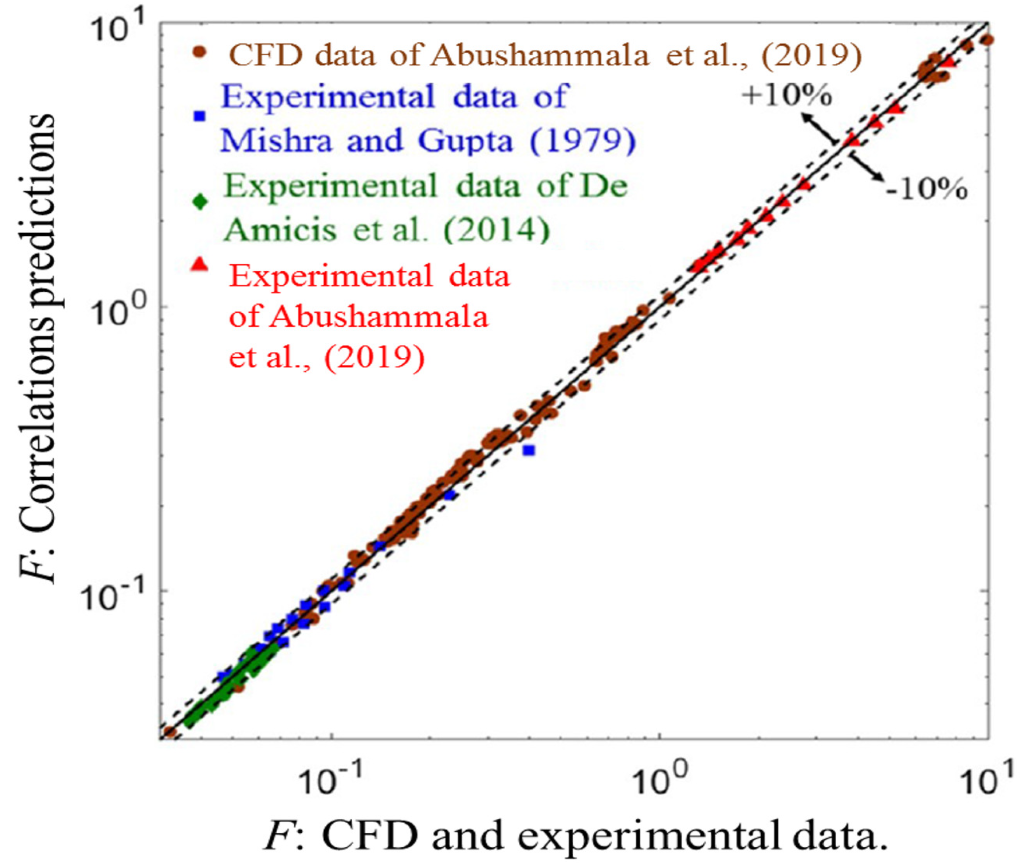
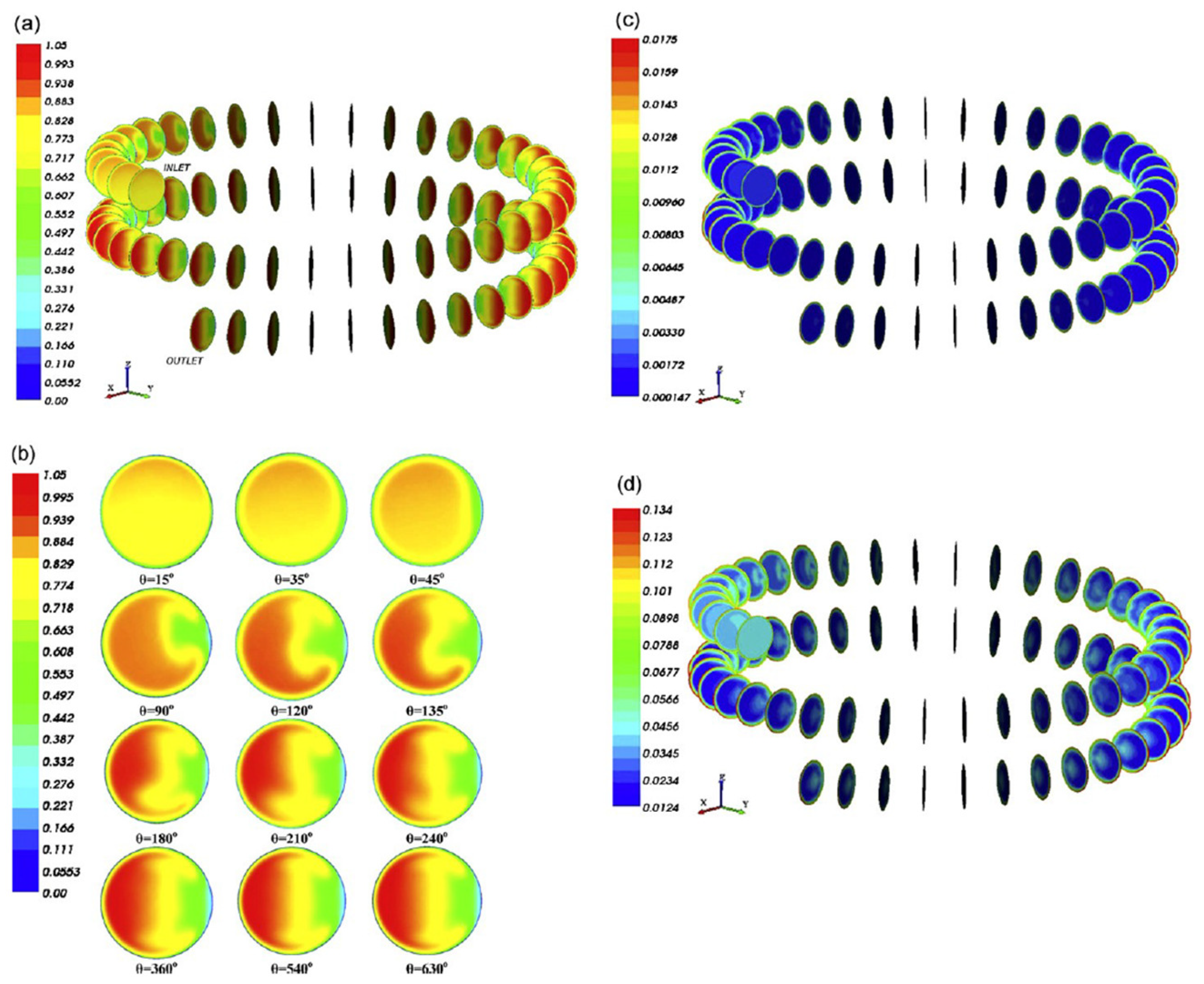
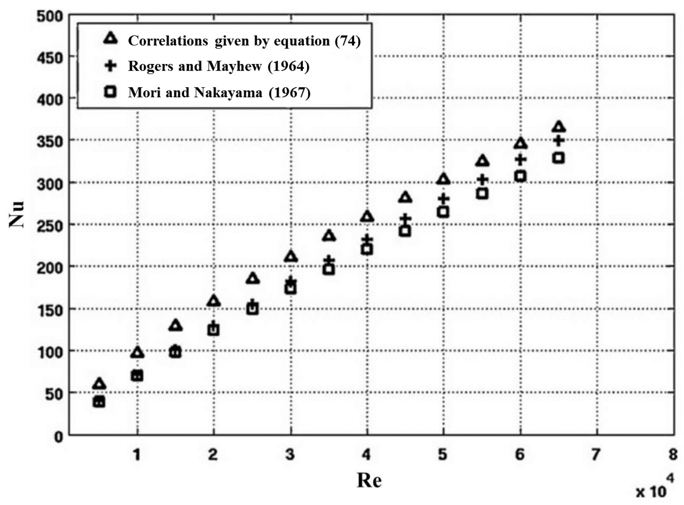
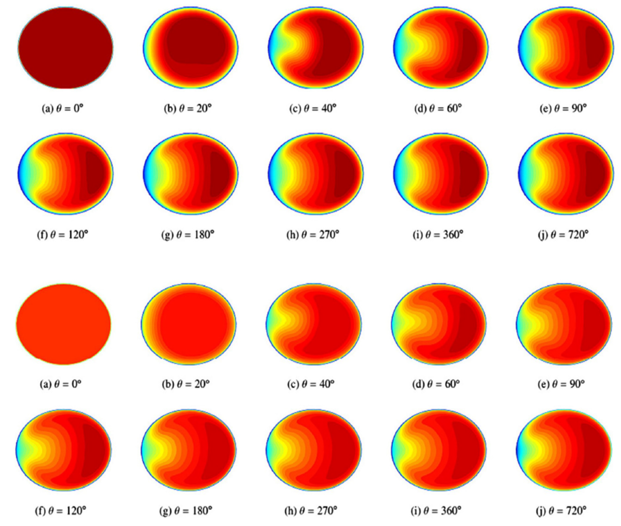
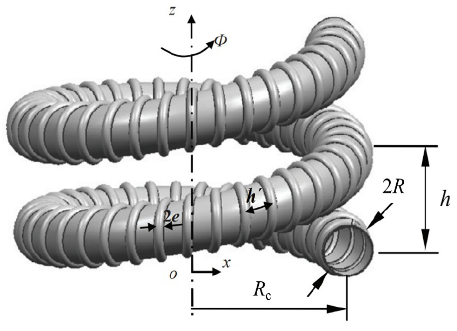
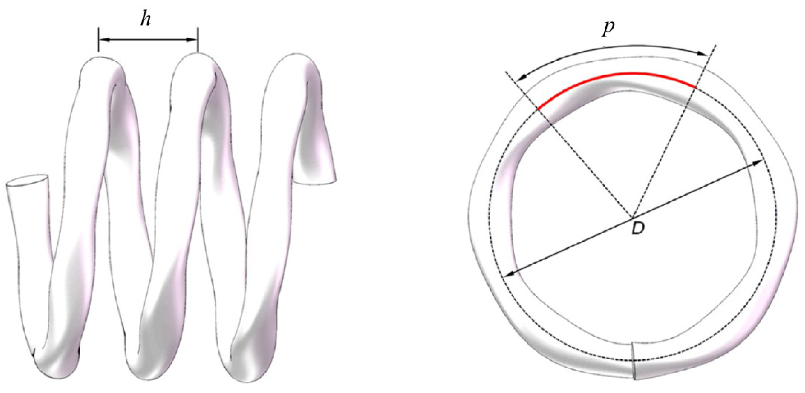
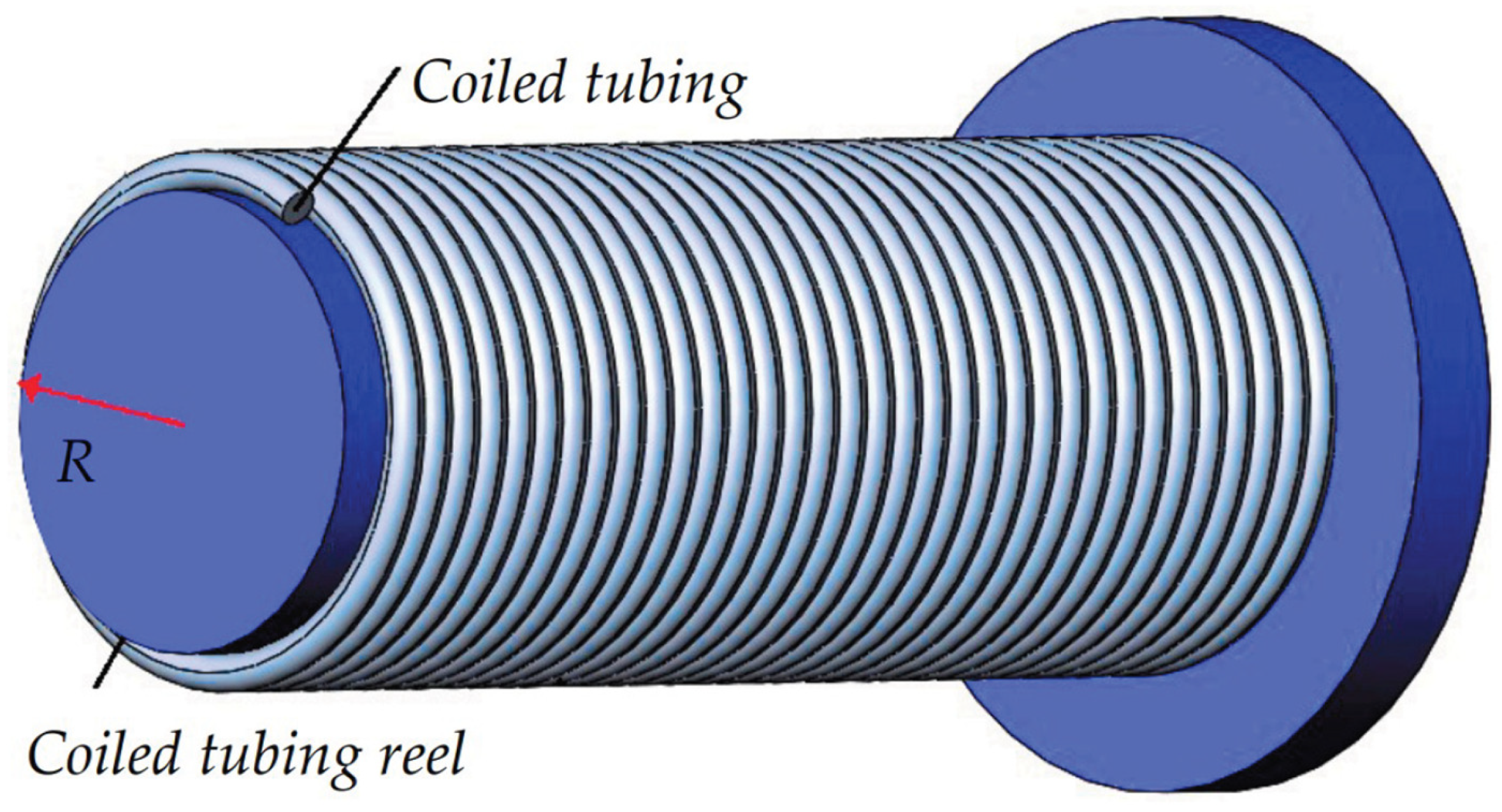
Disclaimer/Publisher’s Note: The statements, opinions and data contained in all publications are solely those of the individual author(s) and contributor(s) and not of MDPI and/or the editor(s). MDPI and/or the editor(s) disclaim responsibility for any injury to people or property resulting from any ideas, methods, instructions or products referred to in the content. |
© 2023 by the authors. Licensee MDPI, Basel, Switzerland. This article is an open access article distributed under the terms and conditions of the Creative Commons Attribution (CC BY) license (https://creativecommons.org/licenses/by/4.0/).
Share and Cite
MDPI and ACS Style
Sigalotti, L.D.G.; Alvarado-Rodríguez, C.E.; Rendón, O. Fluid Flow in Helically Coiled Pipes. Fluids 2023, 8, 308. https://doi.org/10.3390/fluids8120308
AMA Style
Sigalotti LDG, Alvarado-Rodríguez CE, Rendón O. Fluid Flow in Helically Coiled Pipes. Fluids. 2023; 8(12):308. https://doi.org/10.3390/fluids8120308
Chicago/Turabian StyleSigalotti, Leonardo Di G., Carlos E. Alvarado-Rodríguez, and Otto Rendón. 2023. "Fluid Flow in Helically Coiled Pipes" Fluids 8, no. 12: 308. https://doi.org/10.3390/fluids8120308