Modeling of 3D Blood Flows with Physics-Informed Neural Networks: Comparison of Network Architectures

Abstract

Machine learning-based modeling of physical systems has attracted significant interest in recent years. Based solely on the underlying physical equations and initial and boundary conditions, these new approaches allow to approximate, for example, the complex flow of blood in the case of fluid dynamics. Physics-informed neural networks offer certain advantages compared to conventional computational fluid dynamics methods as they avoid the need for discretized meshes and allow to readily solve inverse problems and integrate additional data into the algorithms. Today, the majority of published reports on learning-based flow modeling relies on fully-connected neural networks. However, many different network architectures are introduced into deep learning each year, each with specific benefits for certain applications. In this paper, we present the first comprehensive comparison of various state-of-the-art networks and evaluate their performance in terms of computational cost and accuracy relative to numerical references. We found that while fully-connected networks offer an attractive balance between training time and accuracy, more elaborate architectures (e.g., Deep Galerkin Method) generated superior results. Moreover, we observed high accuracy in simple cylindrical geometries, but slightly poorer estimates in complex aneurysms. This paper provides quantitative guidance for practitioners interested in complex flow modeling using physics-based deep learning.

1. Introduction

Over the last decades, deep neural networks have shown remarkable results in various domains including image segmentation, natural language processing and object recognition, among others. Promising efforts of machine learning-based approaches in scientific computing and especially in solving partial differential equations (PDEs) have been reported in recent years [1,2]. A widely studied PDE is the Navier-Stokes equation, a highly non-linear PDE describing the motion of viscous fluids such as blood. Modeling of vascular flows is a critical component in cardiovascular research, as absolute hemodynamic parameter estimates can be obtained directly from the simulation. Research in risk analysis of intracranial aneurysm ruptures often relies on simulated flow pattern and shear stresses near vessel walls [3]. Since no general analytical solution to the Navier-Stokes equation is known to date, the dynamics of fluids is often modeled via computational fluid dynamics (CFD) solvers (most often based on finite elements or volumes). These numerical solvers benefit from decades of algorithmic fine-tuning, but they predominantly rely on discretized geometries (meshes), which may be challenging to generate for complex irregular geometries and generally imposes a discretization error. Also, their computational cost may be prohibitively high for tackling inverse problems (e.g., in case of unknown boundary conditions or viscosities) [4].

In the late 2010s, deep learning (DL)-based approaches to solve PDEs have been proposed which integrate physical information expressed as PDEs into the training of a neural network. The solution-finding problem is hereby transformed into an optimization problem which attempts to minimize a loss function that contains (a) the residual norms of the governing PDE, (b) the associated initial and boundary conditions and (c) any available labeled (i.e., measurement) data. Physics-informed learning methods are typically mesh-free approaches that operate on batches of randomly sampled points and allow to seamlessly integrate multifidelity/multimodality data into the learning process. Among others, examples of successful DL-based PDE solvers are physics-informed neural networks (PINNs) [5] and the Deep Galerkin Method (DGM) [6].

Fluid mechanics is a prominent topic in physics-based DL [1,7], including PINN studies of blood flows [8,9,10,11,12]. To date, the majority of published reports on DL-based flow modeling relies on fully-connected neural network (FCNN) architectures [9,13,14,15,16,17]. Few other publications report the use of more complex network architectures, such as convolutional neural networks (CNNs) [18,19,20,21] or employ DGMs. While the FCNNs benefit from architectural simplicity, more sophisticated architectures have recently shown superior results in terms of accuracy, efficiency, and memory consumption for specific tasks [7]. Deep learning is generally an active field of research with many network variants and add-ons (e.g., Fourier encoding layers, adaptive activation functions, skip connections) being proposed [22,23]. Although PINNs are still in their early development phase, the interest in physics-informed machine learning is increasing [7,24]. The primary focus of initial PINN reports has been on general feasibility and proof-of-concept. Hence, there is an ongoing need to integrate and evaluate recent DL developments that have shown promising results in other applications. Also, comparing the network architectures found in published results is difficult because of significant variations in simulation domains (2D or 3D, synthetic flow geometries or real blood vessels), fluid characteristics and evaluation metrics.

In this paper we address the applied research question of which network architectures are well suited to learn the complex flow pattern of blood in various geometrical structures. To our knowledge, this is the first systematic report to assess the performance of different state-of-the-art networks, which has been suggested as highly beneficial to deepen the knowledge about PINNs in modeling fluids [6,16].

Physics-Informed Neural Networks

Raissi et al. proposed the concept of PINNs, in which the partial differential equation (PDE) describing the physical system is integrated into a neural network’s loss function. This additional constraint leads to a solution that gradually approaches the one obeying the underlying laws of physics [5,25]. PINNs can directly generate the solution of a physical system solely based on the underlying PDE and initial and boundary conditions without the need for additional data (e.g., measurement data).

In brief, a physical system can be represented by the set of equations

$$\mathcal{N}\left[\mathbf{u}\right]=f\left(\mathbf{x}\right),\mathbf{x}\in \mathsf{\Omega },$$

(1)

$$\mathcal{B}\left[\mathbf{u}\right]=g\left(\mathbf{x}\right),\mathbf{x}\in \partial \mathsf{\Omega },$$

(2)

where $\mathcal{N}[·]$ is a nonlinear differential operator acting on the solution of interest $\mathbf{u}\left(\mathbf{x}\right)$, $\mathsf{\Omega }$ denotes the geometry and $\mathcal{B}[·]$ describes the geometry’s boundary conditions on the boundary $\partial \mathsf{\Omega }$. We consider steady-state systems in this paper, hence, no initial conditions are required.

Following the PINN approach of Raissi et al. [5], we approximate the solution $\mathbf{u}\left(\mathbf{x}\right)$ by a deep neural network ${\mathbf{u}}_{{n}{e}{t}}(\mathbf{x};\theta )$ where $\theta$ represents the set of trainable parameters (i.e., weights and biases). The total loss function is composed of multiple terms: (a) ${\mathcal{L}}_{{P}{D}{E}}$: a loss term given by the PDE’s residuals, (b) ${\mathcal{L}}_{{B}{C}}$: a loss term defined by boundary conditions, and (c) ${\mathcal{L}}_{{d}{a}{t}{a}}$: a loss term calculated from (potentially available) sparse measurement data:

$$\mathcal{L}={\omega }_{{P}{D}{E}}{\mathcal{L}}_{{P}{D}{E}}+{\omega }_{{B}{C}}{\mathcal{L}}_{{B}{C}}\left[+{\omega }_{{d}{a}{t}{a}}{\mathcal{L}}_{{d}{a}{t}{a}}\right]$$

(3)

$${\mathcal{L}}_{{P}{D}{E}}=\frac{1}{N_{{P}{D}{E}}}\sum _{i=1}^{N_{{P}{D}{E}}}{\left.{(\mathcal{N}\left[\mathbf{u}\right]-f\left(\mathbf{x}\right))}^2\right|}_{{\mathbf{x}}_i}$$

(4)

$${\mathcal{L}}_{{B}{C}}=\frac{1}{N_{{B}{C}}}\sum _{j=1}^{N_{{B}{C}}}{\left.{(\mathcal{B}\left[\mathbf{u}\right]-g\left(\mathbf{x}\right))}^2\right|}_{{\mathbf{x}}_j}$$

(5)

$${\mathcal{L}}_{{d}{a}{t}{a}}=\frac{1}{N_{{d}{a}{t}{a}}}\sum _{k=1}^{N_{{d}{a}{t}{a}}}{(\mathbf{u}\left({\mathbf{x}}_k\right)-{\mathbf{u}}_k)}^2$$

(6)

Equation (4) denotes the mean squared residuals of the PDE evaluated at $N_{{P}{D}{E}}$ randomly selected points ${\mathbf{x}}_i$ within the geometry. Similarly, the boundary loss in Equation (5) evaluates the boundary condition on randomly selected points ${\mathbf{x}}_j$ on the geometry’s boundary. In Equation (6), the $N_{{d}{a}{t}{a}}$ points ${\mathbf{x}}_k$ are the measurement points where the solution $\mathbf{u}$ might be known. The data loss term in Equation (3) is bracketed since this term would allow to integrate available measurement data into the PINN training, but was not used throughout this paper. The weight parameters $({\omega }_{{P}{D}{E}},{\omega }_{{B}{C}},{\omega }_{{d}{a}{t}{a}})$ control the weighting of the loss terms. The training of the PINN aims to find the optimal set of network parameters $\theta$ using different optimization algorithms (e.g., Adam [26]), such that the loss function $\mathcal{L}$ is minimized.

2. Methods

2.1. Fluid Model and Geometries

The blood was modeled as an incompressible Newtonian fluid with density $\rho =1050$ kg/m${}^3$ and dynamic viscosity $\mu =3.85$ mPa·s [27]. The dynamic behavior of a fluid is generally described by the Navier-Stokes and continuity equations

$$\rho \left[\frac{\partial \mathbf{u}}{\partial t}+(\mathbf{u}·\nabla )\mathbf{u}\right]-\mu {\nabla }^2\mathbf{u}+\nabla p=0,$$

(7)

$$\nabla ·\mathbf{u}=\mathbf{0}.$$

(8)

In this paper, we consider stationary (i.e., time-independent) systems, therefore the Navier-Stokes equation reduces to

$$\rho \left[(\mathbf{u}·\nabla )\mathbf{u}\right]-\mu {\nabla }^2\mathbf{u}+\nabla p=0.$$

(9)

Here, $\mathbf{u}=\mathbf{u}\left(\mathbf{x}\right)={[u\left(\mathbf{x}\right),v\left(\mathbf{x}\right),w\left(\mathbf{x}\right)]}^{⊺}$ denotes the stationary velocity vector with velocity components $(u,v,w)$, and $p=p\left(\mathbf{x}\right)$ is the pressure field. At the inlet, a parabolic profile for the absolute velocity

$$u_{\mathrm{inlet}}^{\mathrm{abs}}(r)=u_{\max }\left(1-\frac{r^2}{R^2}\right)$$

(10)

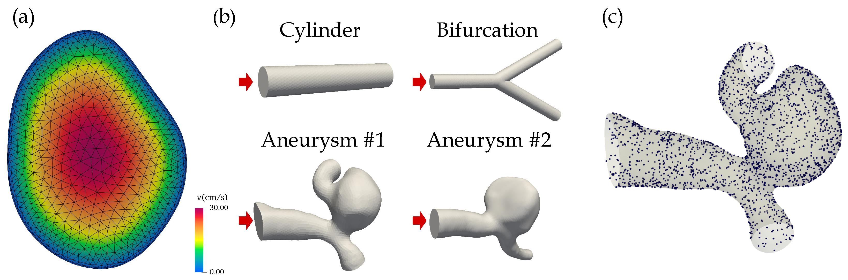
with a realistic, central peak velocity of $u_{\max }=0.3$ m/s was used [27], see Figure 1a. The velocity decreases to zero in radial direction towards the edge, i.e., for each point on the inlet R denotes the distance from the inlet center to the inlet edge on a radial line. The inflow was set perpendicular to the inlet plane. The following boundary conditions were employed: no-slip condition on the geometry walls ($u,v,w=0$) and zero pressure condition at the outlet ($p=0$).

The blood was modeled as a laminar fluid with (geometry-dependent) Reynolds numbers between 80 and 240. The four three-dimensional geometries were: two idealized structures (a cylinder with a radius of 0.5 mm and a length of 5 mm, and a cylindrical bifurcation with a radius of 0.5 mm; Reynolds number of 82) and two realistic intracranial aneurysms (Reynolds numbers of 240), see Figure 1b. The saccular aneurysms located at the middle cerebral artery (MCA) were segmented from digital subtraction angiography (DSA) images.

2.2. Network Architectures

All PINN architectures were implemented in NVIDIA’s Modulus framework v22.03 [28] using Python 3.8.12 and PyTorch 1.11.0. The simulation codes and geometries are available at https://github.com/risc-mi/pinn-blood-flow, accessed on 22 January 2023. In the following, a brief overview of the seven investigated architectures is provided. A more detailed description can be found in the referenced original publications.

2.2.1. Fully Connected Neural Network (FCNN)

In a standard fully-connected architecture, neurons in adjacent layers are connected, whereas neurons inside a single layer are not linked. The network output ${\mathbf{u}}_{{n}{e}{t}}(\mathbf{x};\theta )$ of a FCNN with n layers takes the form

$${\mathbf{u}}_{{n}{e}{t}}(\mathbf{x};\theta )={\mathbf{W}}_n\{{\varphi }_{n-1}\circ {\varphi }_{n-2}\circ ···\circ {\varphi }_1\}\left(\mathbf{x}\right)+{\mathbf{b}}_n,$$

(11)

$${\varphi }_i\left({\mathbf{x}}_i\right)=\sigma ({\mathbf{W}}_i{\mathbf{x}}_i+{\mathbf{b}}_i),$$

(12)

where ${\varphi }_i$ is the i-th layer. ${\mathbf{W}}_i$ and ${\mathbf{b}}_i$ are the weights and biases of the i-th layer, $\mathbf{x}$ is the network’s input and $\sigma$ is the activation function throughout this paper. $\theta$ represents the set of trainable parameters $\theta ={\{{\mathbf{W}}_i,{\mathbf{b}}_i\}}_{i=1}^n$.

2.2.2. Fully Connected Neural Network with Adaptive Activation (FCNNaa)

Adaptive activation functions in various forms have been proposed to improve the training process of neural networks [29,30]. We adopt the approach by Jagtap et al. [31], who integrated a global, trainable, multiplicative parameter $\alpha$ into the activation functions. The trainable parameters are $\theta =\{\alpha ,{\{{\mathbf{W}}_i,{\mathbf{b}}_i\}}_{i=1}^n\}$. The i-th layer of the FCNN from Equation (12) now reads

$${\varphi }_i\left({\mathbf{x}}_i\right)=\sigma (\alpha ·({\mathbf{W}}_i{\mathbf{x}}_i+{\mathbf{b}}_i)).$$

(13)

2.2.3. Fully Connected Neural Network with Skip Connections (FCNNskip)

Skip connections were initially introduced into deep learning for addressing the vanishing gradient problem [32]. They allow information to skip some layer in the neural network, i.e., they feed the output of one layer as the input to the next layers (instead of only the subsequent layer). We applied skip connections every two hidden layers in an FCNN.

2.2.4. Fourier Network (FN)

Fourier networks are an extension of FCNNs and try to reduce spectral biases by employing input encoding [33]. The trend towards low-frequency solutions of neural networks is countered by transforming the input features to a higher dimensional feature space via sinusoidal functions [34,35]. The standard FCNN architecture from Equation (12) is modified by adding an initial Fourier encoding layer ${\varphi }_E$:

$${\mathbf{u}}_{{n}{e}{t}}(\mathbf{x};\theta )={\mathbf{W}}_n\{{\varphi }_{n-1}\circ {\varphi }_{n-2}\circ ···\circ {\varphi }_1\circ {\varphi }_E\}\left(\mathbf{x}\right)+{\mathbf{b}}_n,$$

(14)

$${\varphi }_E=[sin(2\pi {\mathbf{m}}_{\nu }·\mathbf{x});cos(2\pi {\mathbf{m}}_{\nu }·\mathbf{x}{\left)\right]}^T.$$

(15)

In Modulus [28], the Fourier encoding layer is a variation of the one proposed by Tancik et al. [34] and uses a trainable frequency encoding matrix ${\mathbf{m}}_{\nu }$. We used 10 frequencies with the sampling option "axis" in Modulus (i.e., sampling along the axis of the spectral space spanned by all combinations of frequencies in the list [0, …, 9]). The trainable parameters are $\theta =\{{\mathbf{m}}_{\nu },{\{{\mathbf{W}}_i,{\mathbf{b}}_i\}}_{i=1}^n\}$.

2.2.5. Modified Fourier Network (modFN)

In addition to Fourier encoding of the input features, Wang et al. used two additional layers that transform the Fourier features to a learned feature space and transfer the information flow to the other hidden layers via Hadamard multiplications (denoted by ⊙) [36]. The i-th layer reads:

$$\begin{array}{cc}\hfill {\varphi }_i\left({\mathbf{x}}_i\right)=& (1-\sigma ({\mathbf{W}}_i{\mathbf{x}}_i+{\mathbf{b}}_i))\odot \sigma ({\mathbf{W}}_{T_1}{\varphi }_E+{\mathbf{b}}_{T_1})+\hfill \\ & \sigma ({\mathbf{W}}_i{\mathbf{x}}_i+{\mathbf{b}}_i)\odot \sigma ({\mathbf{W}}_{T_2}{\varphi }_E+{\mathbf{b}}_{T_2})\mathrm{for}i>1.\hfill \end{array}$$

(16)

The trainable parameters $\{{\mathbf{W}}_{T_1},{\mathbf{b}}_{T_1},{\mathbf{W}}_{T_2},{\mathbf{b}}_{T_2}\}$ belong to the two additional transformation layers and extend the parameter set of Fourier networks. The Fourier encoding layer ${\varphi }_E$ is given in Equation (15), and the same Fourier encoding parameters were used.

2.2.6. Multiplicative Filter Network (MFN)

MFNs repeatedly apply nonlinear filters (e.g., sinusoid or Gabor wavelets) to the network’s input, then multiply linear functions of these features [37], which relates the network architecture to traditional Fourier and Gabor wavelet transforms. In this paper, we employed the Fourier MFN version:

$$\begin{array}{cc}\hfill & \mathbf{f}(\mathbf{x},{\xi }_i)=sin{(\omega }_i\mathbf{x}+{\varphi }_i)\mathrm{with}{\xi }_i={(\omega }_i,{\varphi }_i),\hfill \\ \hfill & {\varphi }_1=\mathbf{f}(\mathbf{x},{\xi }_1),\hfill \\ \hfill & {\varphi }_{i+1}=\sigma ({\mathbf{W}}_i{\varphi }_i+{\mathbf{b}}_i)\odot f(\mathbf{x},{\xi }_{i+1})\forall i\in \{1,\dots ,n-1\},\hfill \\ \hfill & {\mathbf{u}}_{{n}{e}{t}}(\mathbf{x};\theta )={\mathbf{W}}_n{\varphi }_n+{\mathbf{b}}_n,\hfill \end{array}$$

(17)

where $\mathbf{f}(\mathbf{x},{\xi }_i)$ is the multiplicative Fourier filter, and $\theta$ is again the set of trainable parameters ${\{{\mathbf{W}}_i,{\mathbf{b}}_i,{\xi }_i\}}_{i=1}^n$.

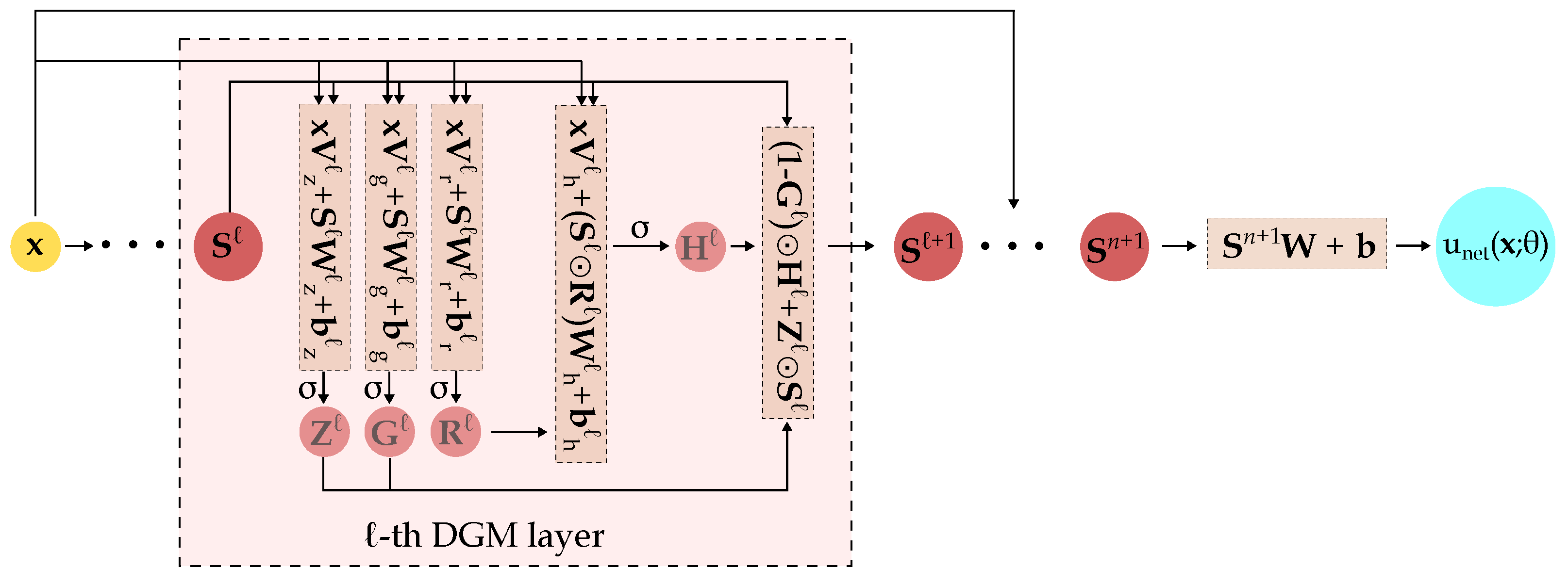
2.2.7. Deep Galerkin Method (DGM)

Sirignano et al. proposed the DGM architecture which is inspired by the Galerkin method but uses a deep neural network instead of a linear combination of basis functions to approximate the PDE’s solution [6]. They proposed the following Long Short-Term Memory (LSTM)-like architecture for the neural network (with $n+1$ hidden layers):

$$\begin{array}{c}\hfill \begin{array}{cc}\hfill & {\mathbf{S}}^1=\sigma (\mathbf{x}{\mathbf{W}}^1+{\mathbf{b}}^1),\hfill \\ \hfill & {\mathbf{Z}}^{\ell }=\sigma (\mathbf{x}{\mathbf{V}}_z^{\ell }+{\mathbf{S}}^{\ell }{\mathbf{W}}_z^{\ell }+{\mathbf{b}}_z^{\ell }),\forall \ell \in \{1,\cdots ,n\},\hfill \\ \hfill & {\mathbf{G}}^{\ell }=\sigma (\mathbf{x}{\mathbf{V}}_g^{\ell }+{\mathbf{S}}^{\ell }{\mathbf{W}}_g^{\ell }+{\mathbf{b}}_g^{\ell }),\forall \ell \in \{1,\cdots ,n\},\hfill \\ \hfill & {\mathbf{R}}^{\ell }=\sigma (\mathbf{x}{\mathbf{V}}_r^{\ell }+{\mathbf{S}}^{\ell }{\mathbf{W}}_r^{\ell }+{\mathbf{b}}_r^{\ell }),\forall \ell \in \{1,\cdots ,n\},\hfill \\ \hfill & {\mathbf{H}}^{\ell }=\sigma (\mathbf{x}{\mathbf{V}}_h^{\ell }+({\mathbf{S}}^{\ell }\odot {\mathbf{R}}^{\ell }){\mathbf{W}}_h^{\ell }+{\mathbf{b}}_h^{\ell }),\forall \ell \in \{1,\cdots ,n\},\hfill \\ \hfill & {\mathbf{S}}^{\ell +1}=(1-{\mathbf{G}}^{\ell })\odot {\mathbf{H}}^{\ell }+{\mathbf{Z}}^{\ell }\odot {\mathbf{S}}^{\ell },\forall \ell \in \{1,\cdots ,n\},\hfill \\ \hfill & {\mathbf{u}}_{{n}{e}{t}}(\mathbf{x};\theta )={\mathbf{S}}^{n+1}\mathbf{W}+\mathbf{b},\hfill \end{array}\end{array}$$

(18)

where $\theta$ is the set of all trainable network parameters

$$\begin{array}{cc}\hfill \theta =& \{{\mathbf{W}}^1,{\mathbf{b}}^1,{\left({\mathbf{V}}_z^{\ell },{\mathbf{W}}_z^{\ell },{\mathbf{b}}_z^{\ell }\right)}_{\ell =1}^n,{\left({\mathbf{V}}_g^{\ell },{\mathbf{W}}_g^{\ell },{\mathbf{b}}_g^{\ell }\right)}_{\ell =1}^n,\hfill \\ & {\left({\mathbf{V}}_r^{\ell },{\mathbf{W}}_r^{\ell },{\mathbf{b}}_r^{\ell }\right)}_{\ell =1}^n,{\left({\mathbf{V}}_h^{\ell },{\mathbf{W}}_h^{\ell },{\mathbf{b}}_h^{\ell }\right)}_{\ell =1}^n,\mathbf{W},\mathbf{b}\}.\hfill \end{array}$$

(19)

The ℓ-th DGM layer takes as input (a) the set of randomly sampled spatial points $\mathbf{x}$ and (b) the output of the previous layer ${\mathbf{S}}^{\ell }$. Since $\mathbf{x}$ enters into the calculations of every intermediate step, the likelihood of vanishing gradients is decreased [38]. Within each DGM layer, a series of transformations (repeated element-wise multiplication of nonlinear functions) are applied to the aforementioned input which should improve the approximation of complex target functions [6]. After running through all layers, the final output is the network’s approximation of the desired function $\mathbf{u}$ evaluated on the set of points $\mathbf{x}$. A schematic of the overall DGM architecture is shown in Figure 2.

Compared to FCNNs, a hidden layer in the DGM network has significantly more parameters because the ℓ-th DGM layer has 8 weight matrices (${\mathbf{V}}_z^{\ell },{\mathbf{V}}_g^{\ell },{\mathbf{V}}_r^{\ell },{\mathbf{V}}_h^{\ell },{\mathbf{W}}_z^{\ell },{\mathbf{W}}_g^{\ell },{\mathbf{W}}_r^{\ell },{\mathbf{W}}_h^{\ell }$) and 4 bias vectors (${\mathbf{b}}_z^{\ell },{\mathbf{b}}_g^{\ell },{\mathbf{b}}_r^{\ell },{\mathbf{b}}_h^{\ell }$) while a standard dense layer only has one weight matrix and one bias vector.

2.3. Network Details

While a broad range of network sizes (i.e., number of layers and neurons per layer) have been described in PINN literature [7], there is a trend towards larger networks. Due to the complexity of our 3D flows we opted to use a network structure of 10 layers with 256 neurons each, which is inspired by previous PINN-based fluid reports [13]. For comparison purposes, the same network size, swish activation functions (with $\beta =1$) [39], exponentially decaying learning rates (Tensorflow parameterization with initial learning rate: 0.0005, decay rate: 0.97, decay steps: 20,000) and Adam optimizers were employed throughout all PINN architectures used in this paper. Equal weights for the loss terms in Equation (3) were used.

The PINN solver used a total of $17\times {10}^6$ randomly sampled spatial points per epoch during the training process. A batch size of 1000 was used, i.e., $17\times {10}^3$ points were employed in each training iteration. Since both the inlet velocity profile and geometry were known, the mass flow at the inlet was well-defined. Using continuity planes placed within the geometry, the mass flow through these planes was calculated via Monte Carlo integration in each training step, and the respective residuals were minimized throughout the training. The boundary conditions and the associated number of sampling points used within each training step are compiled in

Table 1. Boundary conditions used in PINN training. The number of randomly sampled points to evaluate the conditions in the network loss functions is also provided.

	Boundary Condition	#Points
Inlet	Parabolic inlet velocity	2000
Outlet	Zero-pressure: $p=0$	1000
Lateral surface	No-slip: $(u,v,w)=0$	2000
Interior	Navier-Stokes residual	3000
Continuity plane	Mass flow continuity	8000

.

2.4. Computational Fluid Dynamics (CFD)

A proprietary, finite element-based framework (MODSIM) was used to generate ground truths [27,40,41]. MODSIM requires a tetrahedral discretization of the simulation geometry and uses velocity/pressure decoupling [42] with GPU parallelization. Similar boundary conditions as for the PINN training were employed, namely the parabolic inlet velocity profile from Equation (10), no-slip conditions on the wall and zero pressure on the outlets. The artificial mesh surfaces were generated via constructive solid geometry with Netgen [43], whereas the aneurysm geometries were obtained from contrast-enhanced image data (digital subtraction angiography) using a marching cubes algorithm. Some smoothing and mesh optimization was applied, and two boundary layers were added to each CFD mesh to help resolve the physical quantities near the geometry surface (see Figure 1a). Mesh sizes ranged between 2 and 4 million elements, the calculations took 1 to 4 h. All calculations (PINN training and CFD modeling) were performed on a workstation with an Intel i9-11900 CPU, NVIDIA GeForce RTX 3080 Ti and 64 GB RAM.

2.5. Error Analysis

To assess the accuracy/error of the neural networks, we used the mean absolute error (MAE) and standard deviation of absolute errors (STD of AE): The PINNs were evaluated on the reference CFD mesh nodes and the mean (as well as standard deviation) over the point-wise, absolute differences between PINN and CFD solutions was calculated.

We evaluated the error metrics on the following three quantities: pressure, absolute velocity, and wall shear stress. For the cylinder geometry, a comparison with analytically derived values for the pressure (using the Hagen–Poiseuille equation) and the wall shear stress was possible.

3. Results

3.1. Comparison of Accuracy

The errors for the different PINN architectures and geometries against the CFD reference are summarized in

Table 2. Mean absolute errors (MAEs) of the learned solutions for the different geometries and network architectures compared to the CFD references. Bold numbers indicate the best results.

	Cylinder			Bifurcation
	p [Pa]	abs vel [cm/s]	WSS [Pa]	p [Pa]	abs vel [cm/s]	WSS [Pa]
FCNN	0.640 ± 0.422	0.153 ± 0.121	0.085 ± 0.050	0.813 ± 0.338	0.210 ± 0.094	0.169 ± 0.215
FCNNaa	0.642 ± 0.428	0.153 ± 0.122	0.086 ± 0.050	0.826 ± 0.350	0.208 ± 0.091	0.167 ± 0.213
FCNNskip	0.642 ± 0.419	0.153 ± 0.121	0.085 ± 0.050	0.785 ± 0.329	0.203 ± 0.091	0.167 ± 0.218
FN	0.634 ± 0.425	0.154 ± 0.121	0.086 ± 0.050	0.945 ± 0.415	0.214 ± 0.094	0.171 ± 0.212
modFN	0.718 ± 0.425	0.116 ± 0.109	0.071 ± 0.061	0.898 ± 0.395	0.213 ± 0.091	0.173 ± 0.207
MFN	0.663 ± 0.421	0.154 ± 0.122	0.084 ± 0.053	0.628 ± 0.375	0.198 ± 0.138	0.157 ± 0.110
DGM	0.290 ± 0.257	0.107 ± 0.105	0.065 ± 0.054	0.136 ± 0.164	0.118 ± 0.072	0.145 ± 0.220
	Aneurysm $\#1$			Aneurysm $\#2$
	p [Pa]	abs vel [cm/s]	WSS [Pa]	p [Pa]	abs vel [cm/s]	WSS [Pa]
FCNN	0.924 ± 0.622	0.384 ± 0.323	0.607 ± 1.416	2.055 ± 0.672	1.125 ± 1.203	0.419 ± 0.458
FCNNaa	0.968 ± 0.625	0.386 ± 0.323	0.610 ± 1.426	2.056 ± 0.673	1.114 ± 1.201	0.417 ± 0.461
FCNNskip	0.868 ± 0.606	0.364 ± 0.311	0.611 ± 1.428	1.996 ± 0.659	1.123 ± 1.136	0.412 ± 0.433
FN	1.051 ± 0.731	0.512 ± 0.451	0.614 ± 1.412	2.348 ± 0.733	1.214 ± 1.617	0.491 ± 0.655
modFN	0.931 ± 0.647	0.408 ± 0.345	0.611 ± 1.424	2.182 ± 0.685	1.079 ± 1.263	0.441 ± 0.520
MFN	0.732 ± 0.729	0.369 ± 0.340	0.600 ± 1.370	2.203 ± 0.703	1.140 ± 1.391	0.446 ± 0.549
DGM	1.752 ± 1.229	0.363 ± 0.319	0.583 ± 1.380	5.489 ± 1.081	0.557 ± 0.768	0.205 ± 0.338

. For the cylinder, all architectures yielded results that were in good agreement with both the CFD reference (Figure 3) and the analytically derived values. For example, at the inlet, all PINN results deviated less than $1\%$ from the analytical value of $92.4$ Pa. The mean wall shear stress (over the entire lateral surface) differed less than $1\%$ from the analytical value of $4.62$ Pa for all architectures. The lowest errors for all three quantities (pressure, absolute velocity, and wall shear stress) were obtained with the DGM architecture.

Regarding the bifurcation, the smallest errors were again detected with the DGM architecture. The DGM’s error in pressure was roughly a factor five smaller than for MFN, which ranked second best. Slight deviations could be observed in the branching area (see Figure 3), which was most pronounced for the MFN’s absolute velocity estimate.

For both aneurysms, all errors were generally higher compared to the cylinder and bifurcation. The smallest overall errors on absolute velocity and wall shear stresses were obtained for the DGM architecture, although slightly higher velocity errors could be observed for the DGM compared to FCNNs in the central part of aneurysm #1 and the outlet of aneurysm #2. Regarding pressure estimates, the DGM showed the most notable differences to the CFD references, while MFN and FCNNskip yielded the lowest errors.

3.2. Comparison of Training and Inference Runtimes

Table 3. Runtime per training epoch for the different architectures relative to FCNN.

	FCNN	FCNNaa	FCNNskip	FN	modFN	MFN	DGM
Runtime/FCNN	100%	115%	102%	101%	169%	114%	363%

summarizes the computation times per training epoch for the different network architectures relative to the standard FCNN. While FCNNskip and FN required approximately the same time as the simple FCNN, FCNNaa and MFN took around $15\%$ more time to train. DGMs formed the extreme case and took more than a factor 3.6 longer to train than FCNNs.

In absolute numbers, the FCNN training required 140 s per epoch on our hardware, i.e., the training of aneurysm $\#1$ with 2000 training epochs took around 78 h. The inference was fast and took around 1 s for ${10}^6$ points.

Figure 4 shows the mean pressure at the inlet and its trend towards the CFD reference during the training. Overall, increasing the complexity of the geometries required more epochs of network training.

While all FCNN variants and MFN pressure curves quite rapidly approach the CFD value in all geometries, the modFN and the DGM curve exhibit a noticeably delayed convergence compared to the other curves. The modFN (for the cylinder) and the DGM (for the aneurysm $\#2$) architecture even fail to closely approach the respective CFD references.

4. Discussion

The design of the network architecture is a key ingredient of an effective and efficient neural network. Often, successful deep learning approaches exploit some task-related (internal) structure or prior information. Convolutional neural networks have shown remarkable results in image-related tasks, since the convolution operation naturally provides translational invariance and equivariance, which are highly beneficial for object recognition. On the other hand, recurrent neural networks perform particularly well with sequence data due to their ability to respect temporal invariance. However, in many physical systems the underlying symmetry groups are unknown, either because they are highly complex or may even not exist at all.

The Navier-Stokes equation is a prominent PDE in physics-informed machine learning due to broad applications and the general lack of analytic solutions. Blood flow simulations, for example, are essential for research on risk of rupture of intracranial aneurysms and rely on accurate estimates of pressures, velocities, and strains within vessels or near vessel walls.

No invariance-aware network architecture has been identified for the Navier-Stokes equation up to now, hence, the majority of PINN reports rely on generic fully-connected architectures that (supposedly) offer enough representational power for inferring the solution of complex PDEs. Few PINN reports show improvements by tweaking the activation functions, introducing additional transformation layers, or applying specific filters [7]. These reports focus either on a single (new) method in a feasibility study, offer limited comparisons to multiple other network architectures, or employ different error metrics and geometries/dimensions which, overall, impedes comparability.

In this paper, we provide a comprehensive study on the performance of various network architectures in the context of complex 3D blood flow modeling. Using standardized error metrics and simulation geometries, our detailed analysis fills this gap in existing PINN literature. Furthermore, a novel aspect of this paper is that we included network architectures that have shown great results in other deep learning fields (e.g., image representation tasks), but have not yet been used with PINN-based flow modeling.

Overall, all network architectures in this study could infer the qualitative blood flow behaviors within the studied geometries. The solutions were learned by providing just the underlying PDE, boundary conditions, fluid properties and geometry, i.e., no additional measurement (“labeled”) data was provided. We observed that the learned solutions were in closer agreement with the CFD references for the simple geometries (cylinder and bifurcation) than for the aneurysms. This was not surprising as the underlying flow patterns are highly complex (e.g., circulating blood in the aneurysm sac). Moreover, we found notable differences in computational requirements and accuracy across the studied network architectures.

The standard FCNN is the most basic neural network. Theoretically, they offer universal solution representation power despite the simplistic architecture, provided the network has enough neurons [44]. While a major benefit of FCNNs involves their low computational costs (fast training), we found that more elaborate architectures could outperform FCNNs in terms of accuracy, however, at the cost of longer training times. Still, FCNNs achieved mid-tier results throughout all geometries, which renders them quite an efficient architecture when computational resources are scarce.

The activation functions play an important role in the training process of a neural network. Jagtap et al. were the first to introduce activation functions tuned for any number of hidden layers [31]. They showed improved convergence (especially in early training phases), solution robustness and accuracy for solving the nonlinear Klein-Gordon, Burgers and Helmholtz equations. To our knowledge, our work demonstrates the first use of Jagtap’s approach for solving the 3D Navier-Stokes equation. However, we did not observe significant improvements in terms of accuracy and convergence compared to a standard FCNN. Also, Jagtap’s approach of using a global trainable hyperparameter in the activation functions required around $15\%$ more time to train the network. Overall, we found no distinct added value for the FCNNaa architecture compared to FCNNs in our use cases.

Skip connections feed the output of one layer as input to the next layers by skipping some layers in between. They have been described as beneficial in, e.g., Highway Networks [45], ResNets [46] and DSFA-PINN [47] for training deep neural networks. In this paper, we used networks with 10 hidden layers (which is comparably deep for PINNs [7]) and evaluated the benefits of skip connections for the first time for 3D flow modeling. Similar to FCNNaa, the FCNNskip architecture showed comparable accuracy and computational costs to standard FCNNs, with no systematic over-performance.

Tancik et al. have shown that Fourier networks [34] can reduce spectral bias, a frequently observed weakness of fully-connected PINNs [33]. They showed that for some applications adding an initial Fourier feature mapping layer to FCNNs improves the learning of high-frequency or multi-scale functions. Wong et al. have shown that sinusoidal mapping of inputs improved the performance of PINNs across a wide range of forward and inverse modeling problems [48]. Motivated by these findings, we present the first-time application of Fourier networks for 3D blood flow modeling. While we observed similar accuracy compared to FCNNs in the simple cylinder geometry, the results of Fourier networks deteriorated with increasing complexity of the geometry.

Within the modFN architecture (a variation of the Fourier network), the initial Fourier encoding layer is succeeded by a modified FCNN (as proposed by Wang et al. [36]) instead of standard fully-connected layers. Improved multiplicative interactions between varying input dimensions and reduced stiffness of the gradient flow dynamics have been reported by adding two transformation layers. However, we could not observe significant benefits of using a modFN architecture. On the contrary, the accuracy results were among the poorest combined with the second highest computational costs.

Unlike multi-layer networks that achieve representation power through compositional depth, MFNs employ a linear combination of (an exponential number of non-linear) sinusoid or Gabor basis functions on the input. Fathony et al. have shown that MFNs stand up to or outperform other deep architectures (e.g., approaches using Fourier features with ReLU networks) in various image and video (representation) tasks [37]. In this work, we validate the general effectiveness of MFNs also in the context of 3D blood flow modeling. Their training times and accuracies were comparable to FCNNs even in the complex aneurysm structures, but—based on popularity—we regard FCNNs as the more obvious choice of network architecture.

The DGM architecture is based upon the Galerkin methods that seek a reduced-form solution to a PDE as a linear combination of basis functions [6], but uses a deep neural network instead of basis functions. The vast amount of trainable network parameters and multiple element-wise multiplication of nonlinear transformations prolong the training significantly but have been described as beneficial in learning complex functions [6]. In previous works, high efficiency and accuracy have been reported for using DGMs to solve the general Stokes equations in both 2D and 3D cases [49]. Additionally, a feasibility study has shown good agreement with CFD solutions in solving the compressible Navier-Stokes equation [50]. Our findings confirm the significantly increased computational costs (more than a factor 3.5) compared to FCNNs. Regarding accuracy, we obtained the best results for both the cylinder and the bifurcation using the DGM. However, mixed results were achieved for the aneurysm geometries given that the learned velocity and wall shear stress distributions matched the CFD reference closest of all architectures, but the DGMs seemed to struggle with the pressure distributions.

Limitations

(Physics-informed) neural networks are an active field of research with new architectural variants frequently being proposed, and we cannot rule out that other architectures would have performed even better. In particular, we did not include convolutional neural networks in our analysis, although they have shown remarkable results in various domains. The reason is that the classic CNN implementations were originally designed for image-related tasks, where uniformly sampled points on regular Euclidean grids are common. However, on our complex and irregular geometries the basic assumption of shift invariance is not fulfilled, which mathematically prohibits the straightforward use of classic convolutional operations. The emerging domain of geometric deep learning is dedicated to finding ways of adopting CNNs to non-Euclidean spaces [51].

It should be noted that any CFD solution is only an approximation of the complex flow behavior. As the CFD accuracy depends on the numerical scheme and the mesh characteristics, we carefully set up the CFD solver and verified its correctness for the cylinder geometry, where an analytical solution was available.

In this study, we investigated steady-state flow systems described by the time-independent Navier-Stokes equation. Future work may include dynamic systems with time-varying boundary conditions (e.g., pulsed blood flow), which are known to be challenging for PINNs with respect to temporal propagation of initial and boundary conditions.

5. Conclusions

In this study, we applied physics-informed neural networks to model three-dimensional, steady-state blood flows and addressed the practically relevant question which architectures in this rapidly evolving research domain provide the best learning abilities for the complex flow patterns. For this purpose, we performed a comprehensive comparison of various state-of-the-art network architectures and assessed their performance in both idealized and realistic vessel geometries in relation to CFD reference solutions. We found that the applied network architecture has distinct implications on the efficiency and effectiveness of the learning process, i.e., on the speed and accuracy of the training convergence. Adaptive activation functions, skip connections and Fourier input encoding have all been described as beneficial for certain PINN applications. However, we did not observe significant added value compared to a standard fully-connected network. We reported superior results with DGMs, especially in simple geometries, but observed poor pressure estimates in complex aneurysms. Our findings lead to the conclusion that while standard fully-connected networks are an attractive and efficient option (regarding accuracy per unit training time), superior results can be obtained with more elaborate architectures.

As an outlook, we constitute that PDE modeling using deep learning methods is an active field of research and that a future network architecture which intrinsically reflects some underlying physical property/symmetry has the potential to outperform current approaches.

References

- Brunton, S.L.; Noack, B.R.; Koumoutsakos, P. Machine Learning for Fluid Mechanics. Annu. Rev. Fluid Mech. 2020, 52, 477–508. [Google Scholar] [CrossRef] [Green Version]
- Han, J.; Jentzen, A.; E, W. Solving high-dimensional partial differential equations using deep learning. Proc. Natl. Acad. Sci. USA 2018, 115, 8505–8510. [Google Scholar] [CrossRef] [PubMed] [Green Version]
- Zhou, G.; Zhu, Y.; Yin, Y.; Su, M.; Li, M. Association of wall shear stress with intracranial aneurysm rupture: Systematic review and meta-analysis. Sci. Rep. 2017, 7, 5331. [Google Scholar] [CrossRef] [PubMed] [Green Version]
- Cai, S.; Mao, Z.; Wang, Z.; Yin, M.; Karniadakis, G.E. Physics-informed neural networks (PINNs) for fluid mechanics: A review. Acta Mech. Sin. 2021, 37, 1727–1738. [Google Scholar] [CrossRef]
- Raissi, M.; Perdikaris, P.; Karniadakis, G.E. Physics-informed neural networks: A deep learning framework for solving forward and inverse problems involving nonlinear partial differential equations. J. Comput. Phys. 2019, 378, 686–707. [Google Scholar] [CrossRef]
- Sirignano, J.; Spiliopoulos, K. DGM: A deep learning algorithm for solving partial differential equations. J. Comput. Phys. 2018, 375, 1339–1364. [Google Scholar] [CrossRef] [Green Version]
- Cuomo, S.; Di Cola, V.S.; Giampaolo, F.; Rozza, G.; Raissi, M.; Piccialli, F. Scientific Machine Learning Through Physics–Informed Neural Networks: Where we are and What’s Next. J. Sci. Comput. 2022, 92, 88. [Google Scholar] [CrossRef]
- Taebi, A. Deep Learning for Computational Hemodynamics: A Brief Review of Recent Advances. Fluids 2022, 7, 197. [Google Scholar] [CrossRef]
- Arzani, A.; Wang, J.X.; D’Souza, R.M. Uncovering near-wall blood flow from sparse data with physics-informed neural networks. Phys. Fluids 2021, 33, 071905. [Google Scholar] [CrossRef]
- Kissas, G.; Yang, Y.; Hwuang, E.; Witschey, W.R.; Detre, J.A.; Perdikaris, P. Machine learning in cardiovascular flows modeling: Predicting arterial blood pressure from non-invasive 4D flow MRI data using physics-informed neural networks. Comput. Methods Appl. Mech. Eng. 2020, 358, 112623. [Google Scholar] [CrossRef]
- Aliakbari, M.; Mahmoudi, M.; Vadasz, P.; Arzani, A. Predicting high-fidelity multiphysics data from low-fidelity fluid flow and transport solvers using physics-informed neural networks. Int. J. Heat Fluid Flow 2022, 96, 109002. [Google Scholar] [CrossRef]
- Fathi, M.F.; Perez-Raya, I.; Baghaie, A.; Berg, P.; Janiga, G.; Arzani, A.; D’Souza, R.M. Super-resolution and denoising of 4D-Flow MRI using physics-Informed deep neural nets. Comput. Methods Programs Biomed. 2020, 197, 105729. [Google Scholar] [CrossRef]
- Jin, X.; Cai, S.; Li, H.; Karniadakis, G.E. NSFnets (Navier-Stokes flow nets): Physics-informed neural networks for the incompressible Navier-Stokes equations. J. Comput. Phys. 2021, 426, 109951. [Google Scholar] [CrossRef]
- Eivazi, H.; Tahani, M.; Schlatter, P.; Vinuesa, R. Physics-informed neural networks for solving Reynolds-averaged Navier–Stokes equations. Phys. Fluids 2022, 34, 075117. [Google Scholar] [CrossRef]
- Oldenburg, J.; Borowski, F.; Öner, A.; Schmitz, K.P.; Stiehm, M. Geometry aware physics informed neural network surrogate for solving Navier–Stokes equation (GAPINN). Adv. Model. Simul. Eng. Sci. 2022, 9, 8. [Google Scholar] [CrossRef]
- Amalinadhi, C.; Palar, P.S.; Stevenson, R.; Zuhal, L. On Physics-Informed Deep Learning for Solving Navier-Stokes Equations. In Proceedings of the AIAA SCITECH 2022 Forum, San Diego, CA, USA, 3–7 January 2022. [Google Scholar] [CrossRef]
- Raissi, M.; Yazdani, A.; Karniadakis, G.E. Hidden fluid mechanics: Learning velocity and pressure fields from flow visualizations. Science 2020, 367, 1026–1030. [Google Scholar] [CrossRef]
- Ma, H.; Zhang, Y.; Thuerey, N.; Hu, X.Y.; Haidn, O.J. Physics-Driven Learning of the Steady Navier-Stokes Equations using Deep Convolutional Neural Networks. Commun. Comput. Phys. 2022, 32, 715–736. [Google Scholar] [CrossRef]
- Eichinger, M.; Heinlein, A.; Klawonn, A. Stationary Flow Predictions Using Convolutional Neural Networks; Springer: Berlin/Heidelberg, Germany, 2021; pp. 541–549. [Google Scholar] [CrossRef]
- Guo, X.; Li, W.; Iorio, F. Convolutional Neural Networks for Steady Flow Approximation. In Proceedings of the 22nd ACM SIGKDD International Conference on Knowledge Discovery and Data Mining, KDD ’16, San Francisco, CA, USA, 13–17 August 2016; Association for Computing Machinery: New York, NY, USA, 2016; pp. 481–490. [Google Scholar] [CrossRef]
- Gao, H.; Sun, L.; Wang, J.X. PhyGeoNet: Physics-informed geometry-adaptive convolutional neural networks for solving parameterized steady-state PDEs on irregular domain. J. Comput. Phys. 2021, 428, 110079. [Google Scholar] [CrossRef]
- Choudhary, K.; DeCost, B.; Chen, C.; Jain, A.; Tavazza, F.; Cohn, R.; Park, C.W.; Choudhary, A.; Agrawal, A.; Billinge, S.J.L.; et al. Recent advances and applications of deep learning methods in materials science. npj Comput. Mater. 2022, 8, 1–26. [Google Scholar] [CrossRef]
- Markidis, S. The Old and the New: Can Physics-Informed Deep-Learning Replace Traditional Linear Solvers? Front. Big Data 2021, 4. [Google Scholar] [CrossRef]
- Karniadakis, G.E.; Kevrekidis, I.G.; Lu, L.; Perdikaris, P.; Wang, S.; Yang, L. Physics-informed machine learning. Nat. Rev. Phys. 2021, 3, 422–440. [Google Scholar] [CrossRef]
- Raissi, M.; Karniadakis, G.E. Hidden physics models: Machine learning of nonlinear partial differential equations. J. Comput. Phys. 2018, 357, 125–141. [Google Scholar] [CrossRef] [Green Version]
- Kingma, D.P.; Ba, J. Adam: A Method for Stochastic Optimization. In Proceedings of the International Conference on Learning Representations, San Diego, CA, USA, 7–9 May 2015. [Google Scholar] [CrossRef]
- Fenz, W.; Dirnberger, J.; Georgiev, I. Blood Flow Simulations with Application to Cerebral Aneurysms. In Proceedings of the Modeling and Simulation in Medicine Symposium, Pasadena, CA, USA, 3–6 April 2016; Society for Computer Simulation International: San Diego, CA, USA, 2016; p. 3. [Google Scholar] [CrossRef]
- Hennigh, O.; Narasimhan, S.; Nabian, M.A.; Subramaniam, A.; Tangsali, K.; Fang, Z.; Rietmann, M.; Byeon, W.; Choudhry, S. NVIDIA SimNet™: An AI-Accelerated Multi-Physics Simulation Framework. In International Conference on Computational Science, Proceedings of the Computational Science—ICCS 2021: 21st International Conference, Krakow, Poland, 16–18 June 2021; Springer: Berlin/Heidelberg, Germany, 2021; Part V; pp. 447–461. [Google Scholar] [CrossRef]
- Yu, C.C.; Tang, Y.C.; Liu, B.D. An adaptive activation function for multilayer feedforward neural networks. In Proceedings of the 2002 IEEE Region 10 Conference on Computers, Communications, Control and Power Engineering, TENCOM ’02. Beijing, China, 28–31 October 2002; Volume 1, pp. 645–650. [Google Scholar] [CrossRef]
- Qian, S.; Liu, H.; Liu, C.; Wu, S.; Wong, H.S. Adaptive Activation Functions in Convolutional Neural Networks. Neurocomput 2018, 272, 204–212. [Google Scholar] [CrossRef]
- Jagtap, A.D.; Kawaguchi, K.; Karniadakis, G.E. Adaptive activation functions accelerate convergence in deep and physics-informed neural networks. J. Comput. Phys. 2020, 404, 109136. [Google Scholar] [CrossRef] [Green Version]
- He, K.; Zhang, X.; Ren, S.; Sun, J. Deep Residual Learning for Image Recognition. In Proceedings of the 2016 IEEE Conference on Computer Vision and Pattern Recognition (CVPR), Las Vegas, NV, USA, 27–30 June 2016; pp. 770–778. [Google Scholar] [CrossRef] [Green Version]
- Rahaman, N.; Baratin, A.; Arpit, D.; Draxler, F.; Lin, M.; Hamprecht, F.A.; Bengio, Y.; Courville, A. On the Spectral Bias of Neural Networks. In Proceedings of the 36th International Conference on Machine Learning, Long Beach, CA, USA, 9–15 June 2019; Volume 97, pp. 5301–5310. [Google Scholar] [CrossRef]
- Tancik, M.; Srinivasan, P.; Mildenhall, B.; Fridovich-Keil, S.; Raghavan, N.; Singhal, U.; Ramamoorthi, R.; Barron, J.; Ng, R. Fourier Features Let Networks Learn High Frequency Functions in Low Dimensional Domains. In Proceedings of the Advances in Neural Information Processing Systems, Virtual Event. 6–12 December 2020; Curran Associates, Inc.: Red Hook, NY, USA, 2020; Volume 33, pp. 7537–7547. [Google Scholar] [CrossRef]
- Mildenhall, B.; Srinivasan, P.P.; Tancik, M.; Barron, J.T.; Ramamoorthi, R.; Ng, R. NeRF: Representing Scenes as Neural Radiance Fields for View Synthesis. In Proceedings of the Computer Vision—ECCV 2020, Glasgow, UK, 23–28 August 2020; Lecture Notes in Computer Science; Springer International Publishing: Berlin/Heidelberg, Germany, 2020; pp. 405–421. [Google Scholar] [CrossRef]
- Wang, S.; Teng, Y.; Perdikaris, P. Understanding and Mitigating Gradient Flow Pathologies in Physics-Informed Neural Networks. SIAM J. Sci. Comput. 2021, 43, A3055–A3081. [Google Scholar] [CrossRef]
- Fathony, R.; Sahu, A.K.; Willmott, D.; Kolter, J.Z. Multiplicative Filter Networks. In Proceedings of the International Conference on Learning Representations, Virtual Event. 3–7 May 2021. [Google Scholar]
- Al-Aradi, A.; Correia, A.; Naiff, D.; Jardim, G.; Saporito, Y. Solving Nonlinear and High-Dimensional Partial Differential Equations via Deep Learning. arXiv 2018, arXiv:1811.08782. [Google Scholar]
- Ramachandran, P.; Zoph, B.; Le, Q.V. Searching for Activation Functions. arXiv 2017, arXiv:1710.05941. [Google Scholar]
- Fenz, W.; Dirnberger, J.; Watzl, C.; Krieger, M. Parallel simulation and visualization of blood flow in intracranial aneurysms. In Proceedings of the 11th IEEE/ACM International Conference on Grid Computing, Brussels, Belgium, 25–28 October 2010; pp. 153–160. [Google Scholar] [CrossRef]
- Gmeiner, M.; Dirnberger, J.; Fenz, W.; Gollwitzer, M.; Wurm, G.; Trenkler, J.; Gruber, A. Virtual Cerebral Aneurysm Clipping with Real-Time Haptic Force Feedback in Neurosurgical Education. World Neurosurg. 2018, 112, e313–e323. [Google Scholar] [CrossRef]
- Zienkiewicz, O.; Nithiarasu, P.; Codina, R.; Vázquez, M.; Ortiz, P. The characteristic-based-split procedure: An efficient and accurate algorithm for fluid problems. Int. J. Numer. Methods Fluids 1999, 31, 359–392. [Google Scholar] [CrossRef]
- Schöberl, J. NETGEN An advancing front 2D/3D-mesh generator based on abstract rules. Comput. Vis. Sci. 1997, 1, 41–52. [Google Scholar] [CrossRef] [Green Version]
- Blanchard, M.; Bennouna, M.A. The Representation Power of Neural Networks: Breaking the Curse of Dimensionality. arXiv 2021, arXiv:2012.05451. [Google Scholar]
- Srivastava, R.K.; Greff, K.; Schmidhuber, J. Highway Networks. arXiv 2015, arXiv:1505.00387. [Google Scholar]
- Cheng, C.; Zhang, G.T. Deep Learning Method Based on Physics Informed Neural Network with Resnet Block for Solving Fluid Flow Problems. Water 2021, 13, 423. [Google Scholar] [CrossRef]
- Rafiq, M.; Rafiq, G.; Choi, G.S. DSFA-PINN: Deep Spectral Feature Aggregation Physics Informed Neural Network. IEEE Access 2022, 10, 22247–22259. [Google Scholar] [CrossRef]
- Wong, J.C.; Ooi, C.; Gupta, A.; Ong, Y.S. Learning in Sinusoidal Spaces with Physics-Informed Neural Networks. arXiv 2022, arXiv:2109.09338. [Google Scholar]
- Li, J.; Yue, J.; Zhang, W.; Duan, W. The Deep Learning Galerkin Method for the General Stokes Equations. J. Sci. Comput. 2022, 93, 5. [Google Scholar] [CrossRef]
- Matsumoto, M. Application of Deep Galerkin Method to Solve Compressible Navier-Stokes Equations. Trans. Jpn. Soc. Aeronaut. Space Sci. 2021, 64, 348–357. [Google Scholar] [CrossRef]
- Bronstein, M.M.; Bruna, J.; LeCun, Y.; Szlam, A.; Vandergheynst, P. Geometric Deep Learning: Going beyond Euclidean data. IEEE Signal Process. Mag. 2017, 34, 18–42. [Google Scholar] [CrossRef] [Green Version]
Figure 1.
(a) The parabolic velocity profile at the inlet of aneurysm #1. The CFD mesh including the two boundary layers is superimposed. (b) The simulation geometries included two idealized structures (cylinder, bifurcation) and two aneurysms that were segmented from brain DSA images. The inlets are indicated by red arrows. (c) The randomly sampled points on the surface of aneurysm #1 used to evaluate the no-slip boundary condition during PINN training.
Figure 2.
Schematic of the DGM architecture. The detailed operations within the ℓ-th DGM layer are highlighted. is the activation function, ⊙ is the Hadamard (element-wise) multiplication. comprises the network’s trainable parameters, i.e., the various and terms.
Figure 3.
Pressure and absolute velocity distributions across a slice through the geometries for the different network architectures: the cylinder and the bifurcation (-plane through , respectively) and both aneurysms. The absolute errors compared to the CFD reference are also shown.
Figure 4.
Temporal evolution of the mean inlet pressure during the training process of the different network architectures. The dashed line indicates the reference mean inlet pressure obtained from the CFD simulation.