Exact Solutions of Navier–Stokes Equations for Quasi-Two-Dimensional Flows with Rayleigh Friction

Abstract

To solve the problems of geophysical hydrodynamics, it is necessary to integrally take into account the unevenness of the bottom and the free boundary for a large-scale flow of a viscous incompressible fluid. The unevenness of the bottom can be taken into account by setting a new force in the Navier–Stokes equations (the Rayleigh friction force). For solving problems of geophysical hydrodynamics, the velocity field is two-dimensional. In fact, a model representation of a thin (bottom) baroclinic layer is used. Analysis of such flows leads to the redefinition of the system of equations. A compatibility condition is constructed, the fulfillment of which guarantees the existence of a nontrivial solution of the overdetermined system under consideration. A non-trivial exact solution of the overdetermined system is found in the class of Lin–Sidorov–Aristov exact solutions. In this case, the flow velocities are described by linear forms from horizontal (longitudinal) coordinates. Several variants of the pressure representation that do not contradict the form of the equation system are considered. The article presents an algebraic condition for the existence of a non-trivial exact solution with functional arbitrariness for the Lin–Sidorov–Aristov class. The isobaric and gradient flows of a viscous incompressible fluid are considered in detail.

1. Introduction

The study of flows that take place in nature and technical hydrodynamic systems is often characterized by the predominance of the horizontal component of the velocity field over the vertical one [1,2,3,4,5,6,7]. Examples of such flows are large-scale flows both in the ocean and in atmospheres of rotating planets, the convective circulation on the Sun and other stars, the spatial evolution of gas and plasma flows in galaxies, and flows both in magnetized plasma and in thin layers of fluid [1,2,3,4,5,6,7]. In addition, a class of such flows can be implemented in laboratory conditions, in which direct and indirect measurements of various parameters in complex geometry and topologies of flows can be reproduced [1,2,3,4,5,6,7].

The suppression of the vertical velocity component can be due to various reasons. As an illustrative example, we indicate the following factors: the physical competition between regimes of a uniform rigid-body rotation and differential rotation in a fluid, the presence of a magnetic field for an electrically conductive fluid, a pronounced stratification of the force field that induces the movement of a fluid (for example, by a non-uniform density), a small thickness of the fluid layer, and a combination of the phenomena listed above [1,2,3,4,5,6,7]. To describe large-scale incompressible fluid flows moving in thin layers, mathematical models based on the representation of the velocity field by a quasi-two-dimensional flow have proved themselves well [3,4,8,9]. In other words, quasi-two-dimensional flows are two-dimensional in velocity but three-dimensional in geometric coordinates [8,10,11,12].

$$\left(V_x\left(t,x,y,z\right),V_y\left(t,x,y,z\right),0\right)$$

The construction of exact solutions for the Navier–Stokes equations describing quasi-two-dimensional flows is sometimes a more difficult task than finding exact solutions for three-dimensional flows. The main difficulty in finding exact solutions for the velocity field with two nonzero components depending on three coordinates is due to the fact that the reduced equations of motion for an incompressible fluid are overdetermined [8,13,14,15,16,17]. Overdetermination means that the number of equations of the system exceeds the number of functions found from these equations. For isobaric flows of incompressible fluids, exact solutions that take into account the horizontal inhomogeneity of the velocity field were reported in [14,16,17,18]. The study of gradient shear flows in the exact formulation was carried out in [19,20,21,22,23]. For problems of convection, thermal diffusion, and inhomogeneous flows of geophysical hydrodynamics, the exact solutions presented in [16,17,18] were generalized in articles [24,25,26] and in a review [8].

The exact solutions found in [8,13,14,15,16,17,18,19,20,21,22,23,24,25,26] for various force fields can be used to solve boundary value problems with a free boundary [27,28,29,30,31,32]. When describing ocean flows, there is the problem of taking into account the effect of bottom roughness on the structure of the velocity field. In [3], the authors proposed introducing a new force into the Navier–Stokes equations to take into account the roughness of the bottom. This force, which takes into account an external friction according to the Rayleigh law, makes it possible to more accurately describe large-scale flows that take place in natural and technical systems. Note that the Rayleigh friction coefficient depends on both the physical features of the hydrodynamic system and the edge conditions at the flow boundaries [3].

So far, exact solutions for strictly two-dimensional flows (V_x (t,x,y,z), V_y (t,x,y,z), 0) have been considered, and then their stability has been studied [3,4,5,6,7]. Already in pioneering articles [33,34,35] devoted to the study of the Kolmogorov flow with an initial sinusoidal profile, there was a lack of exact solutions for quasi-two-dimensional flows of the form (V_x (t,x,y,z), V_y (t,x,y,z), 0).

We repeat once again that the fundamental difficulty in constructing exact solutions is related to the overdetermination of the system of Navier–Stokes equations together with the incompressibility equation.

This article partially fills the gap in the finding of exact solutions for quasi-two-dimensional flows considered additionally with Rayleigh frictions for various classes of flows. Note that the study of isobaric and gradient flows does not take into account the rotation of the fluid.

Neglecting the influence of the Coriolis force on the fluid flow is due to the intention of the authors to demonstrate the main difficulties associated with the establishment of the solvability condition for the overdetermined system of hydrodynamic equations and the structure of exact solutions, in comparison with the known results obtained from the classical form of the Navier–Stokes equations. This is performed by the authors as they wanted to show the main difficulties that arise when constructing a solvability condition for the overdetermined system of equations that arises during modeling.

2. Problem Statement

Isothermal shear flows of a viscous incompressible fluid are considered here, taking into account the integral influence of the near-bottom boundary layer, which are described by the following system of nonlinear differential equations in partial derivatives [3,36]:

$$\frac{\partial V_x}{\partial t}+V_x\frac{\partial V_x}{\partial x}+V_y\frac{\partial V_x}{\partial y}=-\frac{\partial P}{\partial x}+\mathsf{\nu }\left(\frac{{\partial }^2{V}_x}{\partial x^2}+\frac{{\partial }^2{V}_x}{\partial y^2}+\frac{{\partial }^2{V}_x}{\partial z^2}\right)-\mathsf{\lambda }{V}_x$$

(1)

$$\frac{\partial V_y}{\partial t}+V_x\frac{\partial V_y}{\partial x}+V_y\frac{\partial V_y}{\partial y}=-\frac{\partial P}{\partial y}+\mathsf{\nu }\left(\frac{{\partial }^2{V}_y}{\partial x^2}+\frac{{\partial }^2{V}_y}{\partial y^2}+\frac{{\partial }^2{V}_y}{\partial z^2}\right)-\mathsf{\lambda }{V}_y$$

(2)

$$\frac{\partial P}{\partial z}=0$$

(3)

$$\frac{\partial V_x}{\partial x}+\frac{\partial V_y}{\partial y}=0$$

(4)

Navier–Stokes systems (1)–(4) consist of projections of the momentum equations (Equations (1)–(3)) on the axes of the orthogonal coordinate system and the continuity equation (Equation (4)) for the case of incompressible fluids. In systems (1)–(4), the standard denotation is introduced: V_x(t,x,y,z) and V_y(t,x,y,z) are projections of the velocity vector; P(t,x,y,z) = p/ρ₀ is the pressure p normalized to the fluid density ρ₀; ν is the kinematic viscosity.

A distinctive feature of Equations (1) and (2) is the consideration of the Rayleigh friction force, characterized by the value of the friction coefficient λ. An additional term on the right-hand sides of Equations (1) and (2), containing this coefficient, makes it possible to take into account the bottom roughness. The value of the parameter λ is determined by the edge conditions of the boundary value problem in the geophysical hydrodynamics [3].

Equation (3) means that the pressure does not change with depth. In fact, we are talking about a narrow baroclinic layer existing in the world’s ocean and its internal (near-continental) seas, where the temperature practically does not change.

Among all the equations of the system under consideration, only Equation (3) is isolated, implying that normalized pressure P depends only on part of the spatial coordinates.

However, at the same time, generally speaking, the dependence of the pressure on the other two spatial coordinates and time remains. That is, Equation (3) does not mean the constancy of pressure, but simply narrows the range of parameters on which the pressure value depends:

$$P=P\left(t,x,y\right)$$

(5)

Let us remark that the consideration of shear flows (i.e., flows with a zero vertical velocity) leads to the need to investigate the system of constitutive relations (systems (1)–(4) for compatibility of solutions for separate equations of the aforementioned system). Indeed, the system under the consideration includes four scalar equations for determining three unknown functions—namely, velocities V_x and V_y and pressure P.

To conclude, regarding the solvability condition for systems (1)–(4), we apply the approach presented in [17] for the classical equations of the hydrodynamics of incompressible Newtonian fluids. We differentiate the first equation of the system with respect to x and the second with respect to y, and we sum up the results. As a result of the algebraic manipulations, due to the fact that partial derivatives on analytical functions are always commutative, we obtain the following equation:

$$\frac{\partial }{\partial t}\left(\frac{\partial V_x}{\partial x}+\frac{\partial V_y}{\partial y}\right)+{\left(\frac{\partial V_x}{\partial x}\right)}^2+{\left(\frac{\partial V_y}{\partial y}\right)}^2+V_x\frac{\partial }{\partial x}\left(\frac{\partial V_x}{\partial x}+\frac{\partial V_y}{\partial y}\right)$$

$$+V_y\frac{\partial }{\partial y}\left(\frac{\partial V_x}{\partial x}+\frac{\partial V_y}{\partial y}\right)+2\frac{\partial V_y}{\partial x}\frac{\partial V_x}{\partial y}$$

$$=\mathsf{\nu }\left[\frac{{\partial }^2}{\partial x^2}\left(\frac{\partial V_x}{\partial x}+\frac{\partial V_y}{\partial y}\right)+\frac{{\partial }^2}{\partial y^2}\left(\frac{\partial V_x}{\partial x}+\frac{\partial V_y}{\partial y}\right)+\frac{{\partial }^2}{\partial z^2}\left(\frac{\partial V_x}{\partial x}+\frac{\partial V_y}{\partial y}\right)\right]$$

$$-\frac{{\partial }^{2}P}{\partial x^2}-\frac{{\partial }^{2}P}{\partial y^2}-\mathsf{\lambda }\left(\frac{\partial V_x}{\partial x}+\frac{\partial V_y}{\partial y}\right).$$

(6)

Let us take into account during our calculations that the continuity equation (Equation (4)) in the resulting equation (Equation (6)) simplifies the latter as follows:

$${\left(\frac{\partial V_x}{\partial x}\right)}^2+{\left(\frac{\partial V_y}{\partial y}\right)}^2+2\frac{\partial V_y}{\partial x}\frac{\partial V_x}{\partial y}=-\frac{{\partial }^{2}P}{\partial x^2}-\frac{{\partial }^{2}P}{\partial y^2.}$$

(7)

The derivation of the compatibility condition for solutions of the overdetermined system of Equations (1)–(4), written in the form of (7), does not bring the result closer to constructing the solution itself. First, let us study the solvability of systems (1)–(4) in the Lin–Sidorov–Aristov class of exact solutions [4,8,37,38]. Within the specified class, the velocities V_x and V_y are linear forms of two spatial coordinates with a non-linear arbitrary dependence of the coefficients in these forms on both the third spatial coordinate and time:

$$V_x\left(x,y,z,t\right)=U\left(z,t\right)+u_1\left(z,t\right)x+u_2\left(z,t\right)y,$$

$$V_y\left(x,y,z,t\right)=V\left(z,t\right)+v_1\left(z,t\right)x+v_2\left(z,t\right)y.$$

(8)

The Lin class, with its external simplicity, first allows us to study the behavior of the velocity and acceleration fields. Secondly, it allows us to preserve the nonlinearity of the Navier–Stokes equations and to describe the nonlinear effects observed in real fluids.

We substitute expressions (5) and (8) into the above-considered systems (1)–(4), and we obtain as a result the following:

$$\frac{\partial U}{\partial t}+\frac{\partial u_1}{\partial t}x+\frac{\partial u_2}{\partial t}y+\left(U+u_{1}x+u_{2}y\right)u_1+\left(V+v_{1}x+v_{2}y\right)u_2$$

$$=-\frac{\partial P}{\partial x}+\mathsf{\nu }\left(\frac{{\partial }^{2}U}{\partial z^2}+\frac{{\partial }^2{u}_1}{\partial z^2}x+\frac{{\partial }^2{u}_2}{\partial z^2}y\right)-\mathsf{\lambda }\left(U+u_{1}x+u_{2}y\right),$$

$$\frac{\partial V}{\partial t}+\frac{\partial v_1}{\partial t}x+\frac{\partial v_2}{\partial t}y+\left(U+u_{1}x+u_{2}y\right)v_1+\left(V+v_{1}x+v_{2}y\right)v_2$$

$$=-\frac{\partial P}{\partial x}+\mathsf{\nu }\left(\frac{{\partial }^{2}V}{\partial z^2}+\frac{{\partial }^2{v}_1}{\partial z^2}x+\frac{{\partial }^2{v}_2}{\partial z^2}y\right)-\mathsf{\lambda }\left(V+v_{1}x+v_{2}y\right),$$

$$u_1+v_2=0.$$

(9)

Let us reduce the number of equations and unknown terms in subsystem (9) using the relation

$$v_2=-u_1$$

(10)

between spatial accelerations, which is a direct consequence of the last equation of this system. As a result, we obtain:

$$\left(\frac{\partial U}{\partial t}+U{u}_1+V{u}_2-\mathsf{\nu }\frac{{\partial }^{2}U}{\partial z^2}+\mathsf{\lambda }U\right)+\left(\frac{\partial u_1}{\partial t}+u_1{}^2+u_2{v}_1-\mathsf{\nu }\frac{{\partial }^2{u}_1}{\partial z^2}+\mathsf{\lambda }{u}_1\right)x$$

$$+\left(\frac{\partial u_2}{\partial t}-\mathsf{\nu }\frac{{\partial }^2{u}_2}{\partial z^2}+\mathsf{\lambda }{u}_2\right)y=-\frac{\partial P}{\partial x,}$$

$$\left(\frac{\partial V}{\partial t}+U{v}_1-V{u}_1-\mathsf{\nu }\frac{{\partial }^{2}V}{\partial z^2}+\mathsf{\lambda }V\right)+\left(\frac{\partial v_1}{\partial t}-\mathsf{\nu }\frac{{\partial }^2{v}_1}{\partial z^2}+\mathsf{\lambda }{v}_1\right)x$$

$$-\left(\frac{\partial u_1}{\partial t}-\left(u_1{}^2+u_2{v}_1\right)-\mathsf{\nu }\frac{{\partial }^2{u}_1}{\partial z^2}+\mathsf{\lambda }{u}_1\right)y=-\frac{\partial P}{\partial y}.$$

(11)

Obviously, the left-hand sides of Equation (11) are linear forms in the spatial coordinates x and y. Hence, the right-hand sides of these equations (pressure derivatives with respect to x and y) must also be linear forms of the same coordinates. Therefore, the degree of the polynomial P does not exceed two.

The same conclusion also follows from the compatibility condition. By a direct substitution, one can verify that the compatibility condition for solution (7) for class (8), taking into account condition (9), takes the following form:

$$2\left(u_1{}^2+u_2{v}_1\right)=-\frac{{\partial }^{2}P}{\partial x^2}-\frac{{\partial }^{2}P}{\partial y^2}.$$

(12)

Equation (12) has a function on the left-hand side that depends only on both time t and the vertical coordinate z, which means that the right-hand side of this equation can also be thought to depend only on these parameters. Thus, terms higher than the second degree cannot enter into pressure P.

3. Case 1: The Pressure P Depends Only on Time t

Let us assume that the pressure depends only on the current time t, i.e., represented in the form of

$$P=P_0\left(t\right).$$

(13)

The structure of pressure (13) allows us to consider it as a known function, specified at the boundaries of the fluid flow region. Therefore, what remains is to determine only the components of the velocity field (8).

In addition, due to (13), the compatibility condition (12) takes a simpler form:

$$u_1{}^2+u_2{v}_1=0.$$

(14)

Note that relation (14) was obtained earlier, for example, in [9,17,39], but only steady flows were considered there. In view of the similarity of the form of condition (14) and the compatibility conditions given in [9,17,39], expression (14) is suitable for both steady and unsteady flows.

By virtue of Equations (13) and (14) and the independence of spatial coordinates on each other, the equations of system (11) are reduced to several autonomous equations in the following form:

$$\frac{\partial u_1}{\partial t}-\mathsf{\nu }\frac{{\partial }^2{u}_1}{\partial z^2}+\mathsf{\lambda }{u}_1=0, \frac{\partial u_2}{\partial t}-\mathsf{\nu }\frac{{\partial }^2{u}_2}{\partial z^2}+\mathsf{\lambda }{u}_2=0, \frac{\partial v_1}{\partial t}-\mathsf{\nu }\frac{{\partial }^2{v}_1}{\partial z^2}+\mathsf{\lambda }{v}_1=0,$$

(15)

$$\frac{\partial U}{\partial t}+U{u}_1+V{u}_2-\mathsf{\nu }\frac{{\partial }^{2}U}{\partial z^2}+\mathsf{\lambda }U=0, \frac{\partial V}{\partial t}+U{v}_1-V{u}_1-\mathsf{\nu }\frac{{\partial }^{2}V}{\partial z^2}+\mathsf{\lambda }V=0$$

(16)

Note that all equations of system (15) are isolated. These are linear partial differential equations of the heat conduction type with a source [40].

Let us further introduce into consideration the linear differential operator of a parabolic type:

$$L(\cdot )=\frac{\partial }{\partial t}-\mathsf{\nu }\frac{{\partial }^2}{\partial z^2}+\mathsf{\lambda }$$

System (15) can then be represented as a set of the following operator equations of the same type:

$$L{u}_1=0, L{u}_2=0, L{v}_1=0$$

(17)

After finding the proper solution to system (17), one should return to the integration of the quasi-nonlinear equation (Equation (16)).

Let us consider the special case of a steady flow. The operator L takes the following form:

$$L(\cdot )=-\mathsf{\nu }\frac{{\partial }^2}{\partial z^2}+\mathsf{\lambda }.$$

Consequently, Equation (17) turns into second-order ordinary differential equations with constant coefficients.

The general solution of the homogeneous operator equation Lu = 0 can be easily written out:

$$u\left(z\right)=c_1\exp \left(kz\right)+c_2\exp \left(-kz\right).$$

(18)

where $c_1$ and $c_2$ are constants of integration:

$$k=\sqrt{\frac{\mathsf{\lambda }}{\mathsf{\nu }}}\in R.$$

In view of compatibility condition (14) and the structure of solution (18), the appropriate solution to the system of the operator equation (Equation (17)) is determined by the set of functions:

$$u_1=u\cos \mathsf{\theta }\sin \mathsf{\theta }, u_2=u{\cos }^2\mathsf{\theta }, v_1=-u{\sin }^2\mathsf{\theta },$$

(19)

where u is the function in the form of (18) and θ is some number.

Note that if we put λ = 0 (ignoring the Rayleigh friction), then the characteristic equation corresponding to the differential equation will have a multiple (zero) root. In this case, the solution presented in [9,39] will be obtained. Thus, despite the external similarity of the structure of solution (19) with congruent solutions given in [9,39], we can assume that our current study has generalized the previously presented results.

Then, to completely determine the structure of the velocity field, what remains is to solve the system of two linear equations, which is a simplification of Equation (16) for the case of steady flows under consideration:

$$\mathsf{\lambda }U+U{u}_1+V{u}_2-\mathsf{\nu }\frac{d^{2}U}{d{z}^2}=0, \mathsf{\lambda }V+U{v}_1-V{u}_1-\mathsf{\nu }\frac{d^{2}V}{d{z}^2}=0.$$

(20)

To construct an exact solution of these linear equations with variable coefficients, let us substitute solution (19) for spatial accelerations into Equation (20):

$$\mathsf{\lambda }U+Uu\cos \mathsf{\theta }\sin \mathsf{\theta }+Vu{\cos }^2\mathsf{\theta }-\mathsf{\nu }\frac{d^{2}U}{d{z}^2}=0,$$

$$\mathsf{\lambda }V-Uu{\sin }^2\mathsf{\theta }-Vu\cos \mathsf{\theta }\sin \mathsf{\theta }-\mathsf{\nu }\frac{d^{2}V}{d{z}^2}=0.$$

(21)

Let us consider a special case when sin θ = 0. System (21) is then greatly simplified:

$$\mathsf{\lambda }U+Vu-\mathsf{\nu }\frac{d^{2}U}{d{z}^2}=0, \mathsf{\lambda }V-\mathsf{\nu }\frac{d^{2}V}{d{z}^2}=0.$$

(22)

The last equation can be written as LV = 0, the solution of which has form (18):

$$V=c_3\exp \left(kz\right)+c_4\exp \left(-kz\right).$$

Consequently, the inhomogeneity Vu in the first equation of system (22) will be equal to:

$$Vu=c_1{c}_3\exp \left(2kz\right)+c_2{c}_4\exp \left(-2kz\right)+c_1{c}_4+c_2{c}_3.$$

We look for a particular solution corresponding to it in the form:

$$U_{part}=c_5\exp \left(2kz\right)+c_6\exp \left(-2kz\right)+c_7.$$

By substituting the expression above into the first equation of system (22), we obtain:

$$\mathsf{\lambda }\left(c_5\exp \left(2kz\right)+c_6\exp \left(-2kz\right)+c_7\right)+c_1{c}_3\exp \left(2kz\right)+c_2{c}_4\exp \left(-2kz\right)+c_1{c}_4+c_2{c}_3$$

$$-\mathsf{\nu }\left(4k^2{c}_5\exp \left(2kz\right)+4k^2{c}_6\exp \left(-2kz\right)\right)=0.$$

Taking into account the linear independence of the functions involved, we arrive at the following system of equations:

$$\mathsf{\lambda }{c}_5+c_1{c}_3-4\mathsf{\nu }{c}_5{\left(\sqrt{\frac{\mathsf{\lambda }}{\mathsf{\nu }}}\right)}^2=0, \mathsf{\lambda }{c}_6+c_2{c}_4-4\mathsf{\nu }{c}_6{\left(\sqrt{\frac{\mathsf{\lambda }}{\mathsf{\nu }}}\right)}^2=0,$$

$$\mathsf{\lambda }{c}_7+c_1{c}_4+c_2{c}_3=0.$$

The solution of such systems as above is easy to find:

$$c_5=\frac{c_1{c}_3}{3\mathsf{\lambda }}, c_6=\frac{c_2{c}_4}{3\mathsf{\lambda }}, c_7=-\frac{c_1{c}_4+c_2{c}_3}{\mathsf{\lambda }}.$$

Thus, the final solution to system (22) takes the form:

$$U=c_8\exp \left(kz\right)+c_9\exp \left(-kz\right)+\frac{c_1{c}_3}{3\mathsf{\lambda }}\exp \left(2kz\right)+\frac{c_2{c}_4}{3\mathsf{\lambda }}\exp \left(-2kz\right)-\frac{c_1{c}_4+c_2{c}_3}{\mathsf{\lambda }}$$

$$V=c_3\exp \left(kz\right)+c_4\exp \left(-kz\right).$$

(23)

Let us now return to the analysis of system (21). In the general case, if we consider sin θ ≠ 0, we can multiply the first equation of system (21) by sin θ and the second one by cos θ, and then we can add them as a result. After algebraic transformations, we obtain:

$$\mathsf{\lambda }\left(U\sin \mathsf{\theta }+V\cos \mathsf{\theta }\right)-\mathsf{\nu }\frac{d^2}{d{z}^2}\left(U\sin \mathsf{\theta }+V\cos \mathsf{\theta }\right)=0$$

or

$$L\left(U\sin \mathsf{\theta }+V\cos \mathsf{\theta }\right)=0.$$

The solution of the last equation in view of Equation (18) has the form:

$$U\sin \mathsf{\theta }+V\cos \mathsf{\theta }=c_3\exp \left(kz\right)+c_4\exp \left(-kz\right).$$

(24)

Let us express the velocity U from the resulting relation and substitute it into any equation of system (21) that we are solving here, for example, into the second equation:

$$\mathsf{\lambda }V-\left(c_3\exp \left(kz\right)+c_4\exp \left(-kz\right)-V\cos \mathsf{\theta }\right)u\sin \mathsf{\theta }-Vu\cos \mathsf{\theta }\sin \mathsf{\theta }-\mathsf{\nu }\frac{d^{2}V}{d{z}^2}=0.$$

Having carried out elementary transformations, we obtain an inhomogeneous equation of the form

$$LV=\sin \mathsf{\theta }\left(c_1{c}_3\exp \left(2kz\right)+c_2{c}_4\exp \left(-2kz\right)+c_1{c}_4+c_2{c}_3\right).$$

Relying on the actions performed in the process of searching for a solution to the inhomogeneous equation of system (22) and its final solution (23), we can easily write out the general solution of the last inhomogeneous equation:

$$V=c_5\exp \left(kz\right)+c_6\exp \left(-kz\right)$$

$$-\sin \mathsf{\theta }\left(\frac{c_1{c}_3}{3\mathsf{\lambda }}\exp \left(2kz\right)+\frac{c_2{c}_4}{3\mathsf{\lambda }}\exp \left(-2kz\right)-\frac{c_1{c}_4+c_2{c}_3}{\mathsf{\lambda }}\right).$$

(25)

What remains is to substitute expression (25) into relation (24) to obtain the exact solution describing the behavior of the velocity U:

$$U=\frac{1}{\sin \mathsf{\theta }}\left(c_3\exp \left(kz\right)+c_4\exp \left(-kz\right)-V\cos \mathsf{\theta }\right)$$

$$=\frac{c_3-c_5}{\sin \mathsf{\theta }}\exp \left(kz\right)+\frac{c_4-c_6}{\sin \mathsf{\theta }}\exp \left(-kz\right)$$

$$+\cos \mathsf{\theta }\left(\frac{c_1{c}_3}{3\mathsf{\lambda }}\exp \left(2kz\right)+\frac{c_2{c}_4}{3\mathsf{\lambda }}\exp \left(-2kz\right)-\frac{c_1{c}_4+c_2{c}_3}{\mathsf{\lambda }}\right).$$

(26)

4. Case 2: The Pressure P Is a Linear Form of the Horizontal Coordinates x and y

In this case, the pressure can be represented as the following linear form:

$$P\left(x,y,t\right)=P_0\left(t\right)+x{P}_1\left(t\right)+y{P}_2\left(t\right).$$

(27)

Note that despite adding more terms in the pressure representation (in comparison with form (13)), the compatibility condition in form (14) remains relevant, as the right-hand side of condition (12) for function (27) will be equal to zero.

Let us see how the change in the pressure structure P (27) will affect the form of the equations of system (11). It is easy to verify that by a direct substitution of expression (27), due to the independence of spatial coordinates, system (11) can be reduced to the following system:

$$\frac{\partial u_1}{\partial t}-\mathsf{\nu }\frac{{\partial }^2{u}_1}{\partial z^2}+\mathsf{\lambda }{u}_1=0, \frac{\partial u_2}{\partial t}-\mathsf{\nu }\frac{{\partial }^2{u}_2}{\partial z^2}+\mathsf{\lambda }{u}_2=0, \frac{\partial v_1}{\partial t}-\mathsf{\nu }\frac{{\partial }^2{v}_1}{\partial z^2}+\mathsf{\lambda }{v}_1=0,$$

(28)

$$\frac{\partial U}{\partial t}+U{u}_1+V{u}_2-\mathsf{\nu }\frac{{\partial }^{2}U}{\partial z^2}+\mathsf{\lambda }U=-P_1, \frac{\partial V}{\partial t}+U{v}_1-V{u}_1-\mathsf{\nu }\frac{{\partial }^{2}V}{\partial z^2}+\mathsf{\lambda }V=-P_2.$$

(29)

Comparing systems (15) and (16), and (28) and (29), we notice that the equations for determining the spatial gradients remain unchanged. Let us account for additional terms in expression (27) affecting only the equations for the U and V components. They become inhomogeneous and therefore even more difficult for the exact integration in a general form.

In the particular case of steady flows, the spatial gradients, as in the case of the uniform pressure, will be described by solution (19). So, system (29) will take the form:

$$\mathsf{\lambda }U+Uu\cos \mathsf{\theta }\sin \mathsf{\theta }+Vu{\cos }^2\mathsf{\theta }-\mathsf{\nu }\frac{d^{2}U}{d{z}^2}=-P_1,$$

$$\mathsf{\lambda }V-Uu{\sin }^2\mathsf{\theta }-Vu\cos \mathsf{\theta }\sin \mathsf{\theta }-\mathsf{\nu }\frac{d^{2}V}{d{z}^2}=-P_2.$$

(30)

In this case, the terms on the right-hand side of both equations in Equation (30) are constant. If we assume that sin θ = 0, then, by analogy with the abovementioned case, we arrive to the system of inhomogeneous equations:

$$LU=-P_2-Vu, LV=-P_2.$$

(31)

If sin θ ≠ 0, then, by carrying out transformations similar to those made in the case of a uniform pressure, we again come to an inhomogeneous equation as a result:

$$L\left(U\sin \mathsf{\theta }+V\cos \mathsf{\theta }\right)=-P_1\sin \mathsf{\theta }-P_2\cos \mathsf{\theta }.$$

(32)

Obtaining the solution to Equation (32) above is not difficult, as the inhomogeneity on the right-hand side is constant. This means that we will obtain a linear relationship connecting both homogeneous velocity components.

Expressing further the velocity U in terms of the velocity V (as it was performed above) and substituting into the second equation of system (32), we can, after integration, write out the exact solution for the velocity V. Then, afterward, using the relationship between the components U and V, we can find the exact solution for the velocity U. Calculations and transformations that should be performed according to the above-specified algorithm are not given here, due to two reasons. First, we have already described above the application of the standard technique for finding a particular solution corresponding to the inhomogeneity. Secondly, this entire algorithm has already been considered in sufficient detail using the example of the case of the uniform pressure.

5. Case 3: The Pressure P Is Determined by a Quadratic Dependence on the Coordinates x and y

In this case, the pressure is described by the following sum:

$$P\left(x,y,t\right)=P_0\left(t\right)+x{P}_1\left(t\right)+y{P}_2\left(t\right)+\frac{x^2}{2}{P}_{11}\left(t\right)+xy{P}_{12}\left(t\right)+\frac{y^2}{2}{P}_{22}\left(t\right).$$

The appearance of the quadratic terms in expression (25) (in comparison with form (22)) changes the structure of the compatibility condition (12) (with respect to the condition (14)):

$$P_{11}+P_{22}+2\left(u_1{}^2+u_2{v}_1\right)=0.$$

(33)

In addition, taking into account the terms of the second order also affects the resulting system of equations for the components of the velocity field:

$$\frac{\partial u_1}{\partial t}+u_1{}^2+u_2{v}_1-\mathsf{\nu }\frac{{\partial }^2{u}_1}{\partial z^2}+\mathsf{\lambda }{u}_1=-P_{11}, \frac{\partial u_2}{\partial t}-\mathsf{\nu }\frac{{\partial }^2{u}_2}{\partial z^2}+\mathsf{\lambda }{u}_2=-P_{12},$$

$$\frac{\partial v_1}{\partial t}-\mathsf{\nu }\frac{{\partial }^2{v}_1}{\partial z^2}+\mathsf{\lambda }{v}_1=-P_{12},-\left(\frac{\partial u_1}{\partial t}-\left(u_1{}^2+u_2{v}_1\right)-\mathsf{\nu }\frac{{\partial }^2{u}_1}{\partial z^2}+\mathsf{\lambda }{u}_1\right)=-P_{22},$$

(34)

$$\frac{\partial U}{\partial t}+U{u}_1+V{u}_2-\mathsf{\nu }\frac{{\partial }^{2}U}{\partial z^2}+\mathsf{\lambda }U=-P_1, \frac{\partial V}{\partial t}+U{v}_1-V{u}_1-\mathsf{\nu }\frac{{\partial }^{2}V}{\partial z^2}+\mathsf{\lambda }V=-P_2.$$

(35)

As of now, all equations have become obviously inhomogeneous. This means that the structure of the solution becomes more complicated and the form of some equations has also to be changed.

Let us pay attention to the first and last equations of system (34), presented in the following form:

$$\frac{\partial u_1}{\partial t}-\mathsf{\nu }\frac{{\partial }^2{u}_1}{\partial z^2}+\mathsf{\lambda }{u}_1=-P_{11}-\left(u_1{}^2+u_2{v}_1\right), \frac{\partial u_1}{\partial t}-\mathsf{\nu }\frac{{\partial }^2{u}_1}{\partial z^2}+\mathsf{\lambda }{u}_1=P_{22}+\left(u_1{}^2+u_2{v}_1\right).$$

Both equations are equations for determining the component $u_1$ of the velocity field (8). Note that the left-hand sides of these equations coincide, so the right-hand sides must also match:

$$-P_{11}-\left(u_1{}^2+u_2{v}_1\right)=P_{22}+\left(u_1{}^2+u_2{v}_1\right).$$

Obviously, the last equation coincides with Formula (33). Thus, if relation (33) is satisfied, the first equation in system (34) or the last one can be ignored. The choice of the “discarded” equation is determined conveniently by solving the particular boundary value problem.

Note that in the case of steady flows, the integration of systems (34) and (35) is to be reduced again to solving a set of inhomogeneous equations with linear operator L. The integration of these systems should be carried out completely in a similar way as in case of the uniform pressure, which has been analyzed above in detail.

We perform the appropriate actions to obtain a solution for steady-state flows. In this case, the solution class (8) takes the form:

$$V_x\left(x,y,z\right)=U\left(z\right)+u_1\left(z\right)x+u_2\left(z\right)y,$$

$$V_y\left(x,y,z\right)=V\left(z\right)+v_1\left(z\right)x+v_2\left(z\right)y.$$

(36)

The pressure P is described by a quadric of horizontal coordinates x and y with constant coefficients:

$$P\left(x,y\right)=P_0+x{P}_1+y{P}_2+\frac{x^2}{2}{P}_{11}+xy{P}_{12}+\frac{y^2}{2}{P}_{22}.$$

We construct the solution for systems (34) and (35) for the special case of class (36):

$$V_x\left(x,y,z\right)=U\left(z\right)+u_2\left(z\right)y, V_y\left(x,y,z\right)=V\left(z\right).$$

(37)

The choice of class (37) is explained by the fact that by the invertible transformation of horizontal coordinates (a rotation in the horizontal plane around the origin of coordinates), it is possible to move from class (37) to class (36) using the following expressions:

$$x\to \cos \mathsf{\phi }x+\sin \mathsf{\phi }y, y\to -\sin \mathsf{\phi }x+\cos \mathsf{\phi }y;$$

$$V_x\to \cos \mathsf{\phi }{V}_x+\sin \mathsf{\phi }{V}_y, V_y\to -\sin \mathsf{\phi }{V}_x+\cos \mathsf{\phi }{V}_y$$

(38)

The reverse transition from class (36) to class (37) is also possible with the correct choice of the rotation angle value in expression (38).

So, the component $u_2$ from class (37) can be found from the corresponding equation of system (34):

$$-\mathsf{\nu }{u}_2^{″}+\mathsf{\lambda }{u}_2=-P_{12}.$$

Here, the stroke denotes the derivative by the z coordinate. The solution of the latter equation is easily constructed using the characteristic equation:

$$u_2=A\exp \left(kz\right)+B\exp \left(-kz\right)-\frac{P_{12}}{\mathsf{\lambda }},$$

(39)

as before k = √(λ/ν), A and B are constants of integration.

In this case, system (35) for class (37) becomes weakly related, i.e., an isolated equation is clearly distinguished in it:

$$V^{″}-k^{2}V=\frac{P_2}{\mathsf{\nu }}, U^{″}-k^{2}U=\frac{V{u}_2+P_1}{\mathsf{\nu }}.$$

(40)

The solution of the first equation of system (40) is easily constructed:

$$V=C_1\exp \left(kz\right)+D_1\exp \left(-kz\right)-\frac{P_2}{\mathsf{\lambda }}.$$

(41)

Here, $C_1$ and $D_1$ are constants of integration.

The solution of the second equation of system (40) consists of two parts—the general solution U₁ of a homogeneous equation and a particular solution U₂ of an inhomogeneous equation. Solution U₁ has a structure similar to expression (41):

$$U_1=C_2\exp \left(kz\right)+D_2\exp \left(-kz\right).$$

Here, $C_2$ and $D_2$ are constants of integration.

The form of solution U₂ is determined by the structure of the heterogeneity $V{u}_2+P_1$:

$$\frac{V{u}_2+P_1}{\mathsf{\nu }}=\frac{1}{\mathsf{\nu }}(A{C}_1\exp \left(2kz\right)-\frac{P_{12}{C}_1+P_{2}A}{\mathsf{\lambda }}\exp \left(kz\right)-\frac{P_{12}{D}_1+P_{2}B}{\mathsf{\lambda }}\exp \left(-kz\right)$$

$$\begin{array}{c}\\ \end{array}+B{D}_1\exp \left(-2kz\right)+A{D}_1+B{C}_1+P_1).$$

(42)

In other words, we look for the solution U₂ in the following form:

$$U_2={\mathsf{\alpha }}_1\exp \left(2kz\right)+{\mathsf{\alpha }}_2\exp \left(kz\right)+{\mathsf{\alpha }}_3\exp \left(-kz\right)+{\mathsf{\alpha }}_4\exp \left(-2kz\right)+{\mathsf{\alpha }}_5.$$

(43)

Let us substitute expression (43) into the second equation of system (40):

$$U_2^{″}-k^2{U}_2=3k^2{\mathsf{\alpha }}_1\exp \left(2kz\right)+3k^2{\mathsf{\alpha }}_4\exp \left(-2kz\right)-k^2{\mathsf{\alpha }}_5.$$

(44)

Comparing the coefficients for linearly independent functions exp(2kz), exp(kz), exp(−kz), and exp(−2kz) in expressions (42) and (44), we conclude that the solution exists only if the conditions are met:

$$P_{12}{C}_1+P_{2}A=P_{12}{D}_1+P_{2}B=0.$$

So, as a result, we obtain the following solution for the component U:

$$U=\frac{C_{1}A}{3\mathsf{\lambda }}\exp \left(2kz\right)+C_2\exp \left(kz\right)+D_2\exp \left(-kz\right)+\frac{D_{1}B}{3\mathsf{\lambda }}\exp \left(-2kz\right)-\frac{A{D}_1+B{C}_1+P_1}{\mathsf{\lambda }}.$$

(45)

Now, we can write out the solution for class (37):

$$V_x=U+u_{2}y=\frac{C_{1}A}{3\mathsf{\lambda }}\exp \left(2kz\right)+\left(Ay+C_2\right)\exp \left(kz\right)+\left(By+D_2\right)\exp \left(-kz\right)$$

$$+\frac{D_1{B}_2}{3\mathsf{\lambda }}\exp \left(-2kz\right)-\frac{A{D}_1+B{C}_1+P_1}{\mathsf{\lambda }}.$$

$$V_y=V=C_1\exp \left(kz\right)+D_1\exp \left(-kz\right).$$

(46)

Finally, we apply the rotation transformation (38) to solution (46):

$$V_x=\cos \mathsf{\phi }[\frac{C_{1}A}{3\mathsf{\lambda }}\exp \left(2kz\right)+\left(A\left(-\sin \mathsf{\phi }x+\cos \mathsf{\phi }y\right)+C_2\right)\exp \left(kz\right)$$

$$+\left(B\left(-\sin \mathsf{\phi }x+\cos \mathsf{\phi }y\right)+D_2\right)\exp \left(-kz\right)+\frac{D_1{B}_2}{3\mathsf{\lambda }}\exp \left(-2kz\right)-\frac{A{D}_1+B{C}_1+P_1}{\mathsf{\lambda }}$$

$$-\frac{P_2}{\mathsf{\lambda }}\left(-\sin \mathsf{\phi }x+\cos \mathsf{\phi }y\right)]+\sin \mathsf{\phi }\left[C_1\exp \left(kz\right)+D_1\exp \left(-kz\right)\right],$$

$$V_y=-\sin \mathsf{\phi }[\frac{C_{1}A}{3\mathsf{\lambda }}\exp \left(2kz\right)+\left(A\left(-\sin \mathsf{\phi }x+\cos \mathsf{\phi }y\right)+C_2\right)\exp \left(kz\right)$$

$$+\left(B\left(-\sin \mathsf{\phi }x+\cos \mathsf{\phi }y\right)+D_2\right)\exp \left(-kz\right)+\frac{D_1{B}_2}{3\mathsf{\lambda }}\exp \left(-2kz\right)-\frac{A{D}_1+B{C}_1+P_1}{\mathsf{\lambda }}$$

$$-\frac{P_2}{\mathsf{\lambda }}\left(-\sin \mathsf{\phi }x+\cos \mathsf{\phi }y\right)]+\cos \mathsf{\phi }\left[C_1\exp \left(kz\right)+D_1\exp \left(-kz\right)\right].$$

(47)

Thus, the exact solution of systems (34) and (35) is obtained for steady-state flows within the framework of class (8).

Note that the coefficients before the x and y coordinates in the constructed solution (47) are linear combinations of the functions exp(kz), exp(−kz). In other words, the coefficients before x and y are expressions of the form (39) that satisfy the equations of system (34) for determining the components of the velocity field (8).

6. The Analysis of the Solution

We consider a boundary value problem for a visual illustration of the influence of the friction force on the properties of a steady flow of fluid. The velocity and pressure fields have the following structure:

$$V_x=U\left(z\right), V_y=V\left(z\right), P\left(x,y\right)=P_0+x{P}_1+y{P}_2.$$

(48)

Expressions in (48) are a special case of class (8) for u₁ = u₂ = v₁ = v₂ = 0. System (28) for these values takes the form

$$\mathsf{\lambda }U-\mathsf{\nu }\frac{d^{2}U}{d{z}^2}=-P_1, \mathsf{\lambda }V-\mathsf{\nu }\frac{d^{2}V}{d{z}^2}=-P_2.$$

(49)

If friction is ignored (i.e., assuming λ = 0), equations in Equation (49) describe a flow with a parabolic profile, i.e., Couette–Poiseuille-type flow:

$$U=\frac{P_1}{2\mathsf{\nu }}{z}^2+s_{1}z+s_2, V=\frac{P_2}{2\mathsf{\nu }}{z}^2+s_{3}z+s_4.$$

(50)

However, taking into account the drag coefficient λ fundamentally changes the structure of the solution, and it ceases to be polynomial:

$$U=s_1\exp \left(\sqrt{\frac{\mathsf{\lambda }}{\mathsf{\nu }}}z\right)+s_2\exp \left(-\sqrt{\frac{\mathsf{\lambda }}{\mathsf{\nu }}}z\right)-\frac{P_1}{\mathsf{\lambda }}, V=s_3\exp \left(\sqrt{\frac{\mathsf{\lambda }}{\mathsf{\nu }}}z\right)+s_4\exp \left(-\sqrt{\frac{\mathsf{\lambda }}{\mathsf{\nu }}}z\right)-\frac{P_2}{\mathsf{\lambda }}.$$

(51)

To determine the integration constants s₁, s₂, s₃, and s₄, consider the following boundary conditions. We now assume that the flow occurs in an extended horizontal layer with non-deformable boundaries. At the lower boundary z = 0, the no-slip condition is satisfied:

$$U\left(0\right)=V\left(0\right)=0.$$

(52)

On the upper boundary z = h, the distribution of velocities is given:

$$U\left(h\right)=W\cos \mathsf{\phi },V\left(h\right)=W\sin \mathsf{\phi }.$$

(53)

Under conditions (52) and (53), the exact solution (51) takes the form:

$$U\left(Z\right)=\frac{\exp \left(a\left(1-Z\right)\right)\left(-1+\exp \left(2aZ\right)\right)}{-1+\exp \left(2a\right)}W\cos \mathsf{\phi }$$

$$\hspace{1em}\hspace{1em}\hspace{1em}\hspace{1em}\hspace{1em}\hspace{1em}\hspace{1em}+\frac{\exp \left(-aZ\right)\left(-1+\exp \left(aZ\right)\right)\left(-\exp \left(a\right)+\exp \left(aZ\right)\right)}{1+\exp \left(a\right)}\frac{P_1}{\mathsf{\lambda }},$$

$$V\left(Z\right)=\frac{\exp \left(a\left(1-Z\right)\right)\left(-1+\exp \left(2aZ\right)\right)}{-1+\exp \left(2a\right)}W\sin \mathsf{\phi }$$

$$\hspace{1em}\hspace{1em}\hspace{1em}\hspace{1em}\hspace{1em}\hspace{1em}\hspace{1em}+\frac{\exp \left(-aZ\right)\left(-1+\exp \left(aZ\right)\right)\left(-\exp \left(a\right)+\exp \left(aZ\right)\right)}{1+\exp \left(a\right)}\frac{P_2}{\mathsf{\lambda }}.$$

(54)

In solution (54), the substitutions are introduced:

$$a=\frac{h\sqrt{\mathsf{\lambda }}}{\sqrt{\mathsf{\nu }}}, Z=\frac{z}{h}\in \left[0;1\right].$$

We normalize solution (54) to the characteristic flow velocity W, retaining the notation:

$$U=\frac{\exp \left(a\left(1-Z\right)\right)\left(-1+\exp \left(2aZ\right)\right)}{-1+\exp \left(2a\right)}\cos \mathsf{\phi }$$

$$\hspace{1em}\hspace{1em}\hspace{1em}\hspace{1em}\hspace{1em}\hspace{1em}\hspace{1em}+\frac{\exp \left(-aZ\right)\left(-1+\exp \left(aZ\right)\right)\left(-\exp \left(a\right)+\exp \left(aZ\right)\right)}{1+\exp \left(a\right)}\frac{{\gamma }_1}{\mathrm{Re}\mathsf{\delta }{a}^2},$$

$$V=\frac{\exp \left(a\left(1-Z\right)\right)\left(-1+\exp \left(2aZ\right)\right)}{-1+\exp \left(2a\right)}\sin \mathsf{\phi }$$

$$\hspace{1em}\hspace{1em}\hspace{1em}\hspace{1em}\hspace{1em}\hspace{1em}\hspace{1em}+\frac{\exp \left(-aZ\right)\left(-1+\exp \left(aZ\right)\right)\left(-\exp \left(a\right)+\exp \left(aZ\right)\right)}{1+\exp \left(a\right)}\frac{{\gamma }_2}{\mathrm{Re}\mathsf{\delta }{a}^2}.$$

(55)

Here,

$${\gamma }_1=\frac{h^3{P}_1}{{\mathsf{\nu }}^2},{\gamma }_2=\frac{h^3{P}_2}{{\mathsf{\nu }}^2}, \mathrm{Re}=\frac{Wl}{\mathsf{\nu }}, \mathsf{\delta }=\frac{h}{l},$$

l is a characteristic scale in horizontal x and y coordinates.

Note that the following passage to the limit is performed for solution (55):

$$\underset{a=\frac{h\sqrt{\mathsf{\lambda }}}{\sqrt{\mathsf{\nu }}}\to 0}{\lim }U=\frac{2\mathrm{Re}\mathsf{\delta }\cos \mathsf{\phi }+{\gamma }_1\left(-1+Z\right)}{2\mathrm{Re}\mathsf{\delta }}Z,$$

$$\underset{a=\frac{h\sqrt{\mathsf{\lambda }}}{\sqrt{\mathsf{\nu }}}\to 0}{\lim }V=\frac{2\mathrm{Re}\mathsf{\delta }\sin \mathsf{\phi }+{\gamma }_2\left(-1+Z\right)}{2\mathrm{Re}\mathsf{\delta }}Z.$$

(56)

Solution (56) describes the Couette–Poiseuille flow profile, and if we additionally put γ₁ = 0 and γ₂ = 0 (i.e., ignore the possible pressure drop in horizontal directions), then there will be a classic linear Couette profile:

$$U=\cos \mathsf{\phi }Z, V=\sin \mathsf{\phi }Z.$$

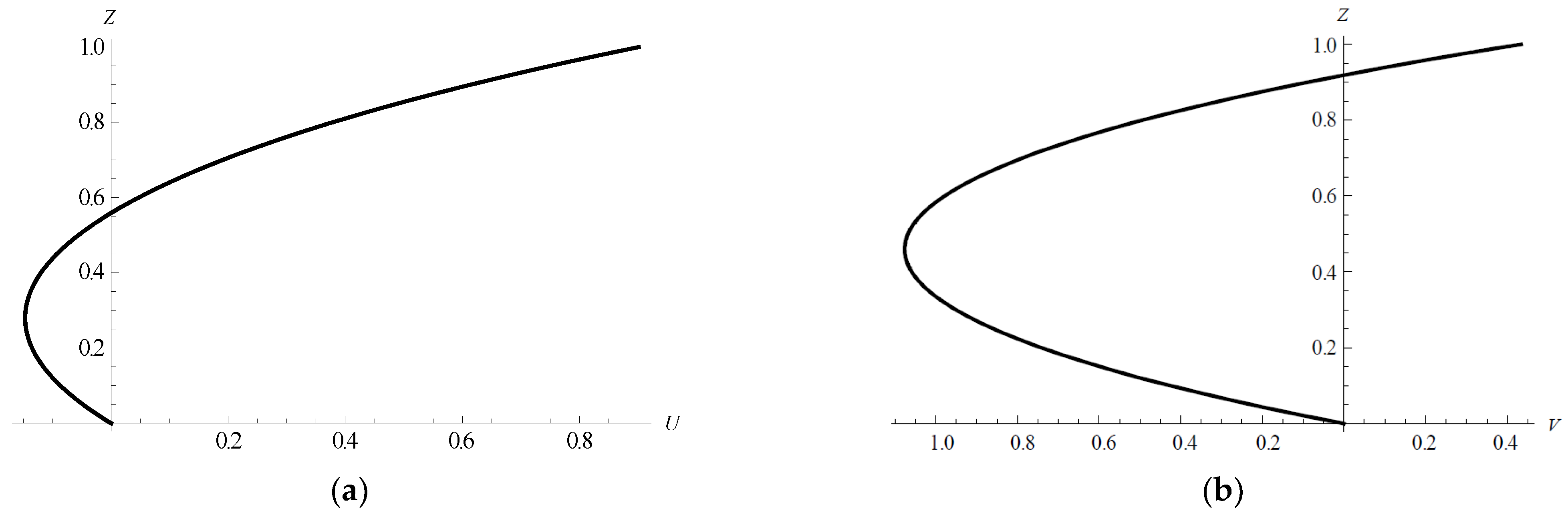
The velocity field profile (55) is determined by the interaction of two nonlinear flows, one of which is induced by the movement of the upper boundary, the other by the pressure difference (Figure 1). The hodograph of the velocity vector is shown in Figure 2.

Note that the characteristic value a = √2 was used in the calculations. This value results from the expression λ = 2ν/h² [3]. For comparison, Figure 3 shows the profiles of the velocity field determined by exact solution (50) taking into account boundary conditions (52) and (53).

As can be seen from Figure 3, there is a qualitative similarity of the hodographs: there is a return section on both curves, and both curves intersect the axes, which indicates the occurrence of countercurrents, but significant differences in quantitative estimates are visible.

7. Conclusions

In this article, the problem of the overdetermination for the system of equations used to describe shear flows of viscous fluids, additionally introducing into consideration the Rayleigh friction, is studied. The reduced systems of equations for the velocity field that is linear in the x and y coordinates are given. It is shown that the pressure should be a polynomial depending on the aforementioned coordinates, and the degree of such polynomials does not exceed two. Conditions for avoiding the abovementioned overdetermination are derived for the constructed class of solutions. It is shown that the form of the compatibility condition for solutions of such systems depends on the chosen structure of the pressure field. It is also shown that this structure affects the form of equations for determining the components of the velocity field. Among other findings, new nontrivial exact solutions (within the suggested class) that take into account the Rayleigh friction are constructed for the particular case of steady flows.

References

- Ekman, V.W. On the influence of the Earth’s rotation on ocean-currents. Ark. Mat. Astron. Fys. 1905, 2, 1874–1954. [Google Scholar]
- Pedlosky, J. Geophysical Fluid Dynamics; Springer: Berlin, Germany; New York, NY, USA, 1987. [Google Scholar]
- Dolzhansky, F.V.; Krymov, V.A.; Manin, D.Y. Stability and vortex structures of quasi-two-dimensional shear flows. Phys. Usp. 1990, 33, 495–520. [Google Scholar] [CrossRef]
- Aristov, S.N. Eddy Currents in Thin Liquid Layers. Ph.D. Thesis, Institute of Automation and Control Processes, Vladivostok, Russia, 1990. [Google Scholar]
- Drazin, P.G.; Reid, W.H. Hydrodynamic Stabilityi; Cambridge University Press: Cambridge, UK, 1981. [Google Scholar]
- Drazin, P.G.; Riley, N. The Navier–Stokes Equations: A Classification of Flows and Exact Solutions; Cambridge University Press: Cambridge, UK, 2006. [Google Scholar]
- Nezlin, M.V. Rossby solitons (Experimental investigations and laboratory model of natural vortices of the Jovian Great Red Spot type). Sov. Phys. Usp. 1986, 29, 807–842. [Google Scholar] [CrossRef]
- Ershkov, S.V.; Prosviryakov, E.Y.; Burmasheva, N.V.; Christianto, V. Towards understanding the algorithms for solving the Navier–Stokes equations. Fluid Dyn. Res. 2021, 53, 044501. [Google Scholar] [CrossRef]
- Burmasheva, N.V.; Prosviryakov, E.Y. A class of exact solutions for two-dimensional equations of geophysical hydrodynamicswith two Coriolis parameters. Izv. Irkutsk. Gos. Univ. Ser. Mat. 2020, 32, 33–48. [Google Scholar]
- Ladyzhenskaya, O.A. On nonstationary Navier–Stokes equations. Vestn. Leningr. Univ. 1958, 19, 9–18. [Google Scholar]
- Ladyzhenskaya, O.A. On some gaps in two of my papers on the Navier–Stokes equations and the way of closing them. J. Math. Sci. 2003, 115, 2789–2791. [Google Scholar] [CrossRef]
- Pukhnachev, V.V. Symmetries in the Navier–Stokes equations. Uspekhi Mekhaniki 2006, 1, 6–76. [Google Scholar]
- Aristov, S.N.; Knyazev, D.V.; Polyanin, A.D. Exact solutions of the Navier–Stokes equations with the linear dependence of velocity components on two space variables. Theor. Found. Chem. Eng. 2009, 43, 642–662. [Google Scholar] [CrossRef]
- Ershkov, S.; Prosviryakov, E.; Leshchenko, D. Exact solutions for isobaric inhomogeneous Couette flows of a vertically swirling fluid. J. Appl. Computat. Mech. 2023, 9, 521–528. [Google Scholar]
- Baranovskii, E.S.; Burmasheva, N.V.; Prosviryakov, E.Y. Exact solutions to the Navier–Stokes equations with couple stresses. Symmetry 2021, 13, 1355. [Google Scholar] [CrossRef]
- Aristov, S.N.; Prosviryakov, E.Y. Unsteady layered vortical fluid flows. Fluid Dyn. 2016, 51, 148–154. [Google Scholar] [CrossRef]
- Zubarev, N.M.; Prosviryakov, E.Y. Exact solutions for layered three-dimensional nonstationary isobaric flows of a viscous incompressible fluid. J. Appl. Mech. Tech. Phys. 2019, 60, 1031–1037. [Google Scholar] [CrossRef]
- Burmasheva, N.V.; Prosviryakov, E.Y. Exact solutions to Navier–Stokes equations describing a gradient nonuniform unidirectional vertical vortex fluid flow. Dynamics 2022, 2, 175–186. [Google Scholar] [CrossRef]
- Bogoyavlenskij, O. The new effect of oscillations of the total angular momentum vector of viscous fluid. Phys. Fluids 2022, 34, 083108. [Google Scholar] [CrossRef]
- Bogoyavlenskij, O. The new effect of oscillations of the total kinematic momentum vector of viscous fluid. Phys. Fluids 2022, 34, 123104. [Google Scholar] [CrossRef]
- Prosviryakov, E.Y. Layered gradient stationary flow vertically swirling viscous incompressible fluid. CEUR Workshop Proc. 2016, 1825, 164–172. [Google Scholar]
- Ershkov, S.V.; Shamin, R.V. On a new type of solving procedure for Laplace tidal equation. Phys. Fluids 2018, 30, 127107. [Google Scholar] [CrossRef] [Green Version]
- Ershkov, S.V. Non-stationary creeping flows for incompressible 3D Navier–Stokes equations. Eur. J. Mech. B Fluids 2017, 61, 154–159. [Google Scholar] [CrossRef]
- Bashurov, V.V.; Prosviryakov, E.Y. Steady thermo-diffusive shear Couette flow of incompressible fluid. Velocity field analysis. Vestn. SamGTU-Seriya-Fiz.-Mat. Nauk. 2021, 25, 781–793. [Google Scholar] [CrossRef]
- Burmasheva, N.V.; Prosviryakov, E.Y. Exact solutions to the Navier–Stokes equations describing stratified fluid flows. Vestn. SamGTU-Seriya-Fiz.-Mat. Nauk. 2021, 25, 491–507. [Google Scholar] [CrossRef]
- Burmasheva, N.V.; Prosviryakov, E.Y. Exact solutions to the Oberbeck–Boussinesq equations for shear flows of a viscous binary fluid with allowance made for the Soret effect. Bull. Irkutsk. State Univ.-Ser. Math. 2021, 37, 17–30. [Google Scholar] [CrossRef]
- Ingel, L.K.; Kalashnik, M.V. Nontrivial features in the hydrodynamics of seawater and other stratified solutions. Phys. Usp. 2012, 55, 356–381. [Google Scholar] [CrossRef]
- Öz, Y. Rigorous investigation of the Navier–Stokes momentum equations and correlation tensors. AIP Adv. 2021, 11, 055009. [Google Scholar] [CrossRef]
- Wang, C.Y. Exact solutions of the unsteady Navier–Stokes equations. Appl. Mech. Rev. 1989, 42, 269–282. [Google Scholar] [CrossRef]
- Wang, C.Y. Exact solutions of the steady-state Navier–Stokes equations. Annu. Rev. Fluid Mech. 1991, 23, 159–177. [Google Scholar] [CrossRef]
- Pukhnachev, V.V. Strip deformation problem in three models of hydrodynamics. Theoret. Math. Phys. 2022, 211, 701–711. [Google Scholar] [CrossRef]
- Korobkov, M.V.; Pileckas, K.; Pukhnachov, V.V.; Russo, R. The flux problem for the Navier–Stokes equations. Russ. Math. Surv. 2014, 69, 1065–1122. [Google Scholar] [CrossRef]
- Meshalkin, L.D.; Sinai, I.G. Investigation of the stability of a stationary solution of a system of equations for the plane movement of an incompressible viscous liquid. J. Appl. Math. Mech. 1961, 25, 1700–1705. [Google Scholar] [CrossRef]
- Obukhov, A.M. Kolmogorov flow and laboratory simulation of it. Russ. Math. Surv. 1983, 38, 113–126. [Google Scholar] [CrossRef] [Green Version]
- Sivashinsky, G.I. Weak turbulence in periodic flows. Phys. D Nonlinear Phenom. 1985, 17, 243–255. [Google Scholar] [CrossRef]
- Kalashnik, M.V.; Kurgansky, M.V.; Chkhetiani, O.G. Baroclinic instability in geophysical fluid dynamics. Phys. Usp. 2022, 65, 1039–1070. [Google Scholar] [CrossRef]
- Lin, C.C. Note on a class of exact solutions in magneto-hydrodynamics. Arch. Ration. Mech. Anal. 1958, 1, 391–395. [Google Scholar] [CrossRef]
- Sidorov, A.F. Two classes of solutions of the fluid and gas mechanics equations and their connection to traveling wave theory. J. Appl. Mech. Tech. Phys. 1989, 30, 197–203. [Google Scholar] [CrossRef]
- Burmasheva, N.V.; Prosviryakov, E.Y. Exact solutions for steady convective layered flows with a spatial acceleration. Rus. Math. 2021, 65, 8–16. [Google Scholar] [CrossRef]
- Polyanin, A.D.; Zaitsev, V.F. Handbook of Nonlinear Partial Differential Equations; Chapman & Hall; CRC Press: Boca Raton, FL, USA, 2004. [Google Scholar]
Figure 1.
(a) Velocity profile U; (b) Velocity profile V.
Figure 2.
Velocity vector hodograph.
Figure 3.
Velocity vector hodograph with friction (solid line) and without friction (dashed line).
Disclaimer/Publisher’s Note: The statements, opinions and data contained in all publications are solely those of the individual author(s) and contributor(s) and not of MDPI and/or the editor(s). MDPI and/or the editor(s) disclaim responsibility for any injury to people or property resulting from any ideas, methods, instructions or products referred to in the content. |
© 2023 by the authors. Licensee MDPI, Basel, Switzerland. This article is an open access article distributed under the terms and conditions of the Creative Commons Attribution (CC BY) license (https://creativecommons.org/licenses/by/4.0/).
Share and Cite
MDPI and ACS Style
Burmasheva, N.; Ershkov, S.; Prosviryakov, E.; Leshchenko, D. Exact Solutions of Navier–Stokes Equations for Quasi-Two-Dimensional Flows with Rayleigh Friction. Fluids 2023, 8, 123. https://doi.org/10.3390/fluids8040123
AMA Style
Burmasheva N, Ershkov S, Prosviryakov E, Leshchenko D. Exact Solutions of Navier–Stokes Equations for Quasi-Two-Dimensional Flows with Rayleigh Friction. Fluids. 2023; 8(4):123. https://doi.org/10.3390/fluids8040123
Chicago/Turabian StyleBurmasheva, Natalya, Sergey Ershkov, Evgeniy Prosviryakov, and Dmytro Leshchenko. 2023. "Exact Solutions of Navier–Stokes Equations for Quasi-Two-Dimensional Flows with Rayleigh Friction" Fluids 8, no. 4: 123. https://doi.org/10.3390/fluids8040123