Article

Thin Film Evaporation Modeling of the Liquid Microlayer Region in a Dewetting Water Bubble

1
Department of Mechanical and Materials Engineering, University of Cincinnati, P.O. Box 210072, Cincinnati, OH 45221, USA
2
Department of Mechanical, Aerospace & Civil Engineering, School of Engineering, University of Manchester, Manchester M13 9PL, UK
3
Department of Nuclear Engineering, Kyung Hee University, Yongin 17104, Republic of Korea
*
Author to whom correspondence should be addressed.
Fluids 2023, 8(4), 126; https://doi.org/10.3390/fluids8040126
Submission received: 7 March 2023 / Revised: 27 March 2023 / Accepted: 31 March 2023 / Published: 4 April 2023
(This article belongs to the Special Issue Contact Line Dynamics and Droplet Spreading)

Abstract

:
Understanding the mechanism of bubble growth is crucial to modeling boiling heat transfer and enabling the development of technological applications, such as energy systems and thermal management processes, which rely on boiling to achieve the high heat fluxes required for their operation. This paper presents analyses of the evaporation of “microlayers”, i.e., ultra-thin layers of liquid present beneath steam bubbles growing at the heated surface in the atmospheric pressure nucleate of boiling water. Evaporation of the microlayer is believed to be a major contributor to the phase change heat transfer, but its evolution, spatio-temporal stability, and impact on macroscale bubble dynamics are still poorly understood. Mass, momentum, and energy transfer in the microlayer are modeled with a lubrication theory approach that accounts for capillary and intermolecular forces and interfacial mass transfer. The model is embodied in a third-order nonlinear film evolution equation, which is solved numerically. Variable wall-temperature boundary conditions are applied at the solid–liquid interface to account for conjugate heat transfer due to evaporative heat loss at the liquid–vapor interface. Predictions obtained with the current approach compare favorably with experimental measurements of microlayer evaporation. By comparing film profiles at a sequence of times into the ebullition cycle of a single bubble, likely values of evaporative heat transfer coefficients were inferred and found to fall within the range of previously reported estimates. The result suggests that the coefficients may not be a constant, as previously assumed, but instead something that varies with time during the ebullition cycle.

1. Introduction

The phase change flux from a thin film is several orders of magnitude greater than the bulk liquid [1]. Hence, researchers have recently increased the use of thin films in high-performance phase change heat transfer devices such as spray coolers, heat pipes, capillary pumped loops, and grooved evaporators [2]. Even in a nucleate boiling scenario, a thin film is momentarily formed underneath a bubble just prior to departure and is generally referred to as the “microlayer” (Figure 1). The superheated thin film forms a conduction path between the solid–liquid interface (heated wall) and the liquid–vapor interface, where evaporation takes place. This results in thermal resistance and is critical to overall heat transfer and fluid flow. The evaporation from this superheated liquid film causes the bubble to grow while diminishing film thickness at the same time. As the bubble grows in size, a net upward force develops due to the density gradient and vapor recoil. The upward forces finally overcome surface tension when the bubble becomes large enough to detach itself from the heated surface. As seen in Figure 1, the liquid region can be delineated into three main parts based on the dominant pressure component. In the bulk region, the surface/capillary force is generally dominant and influences the macroscale bubble shape. However, in the nanoscale adsorbed (also referred to as a ‘precursor’) film region, intermolecular forces have a dominating effect and are characterized by a disjoining pressure [3]. Thus, the combined action of the disjoining pressure and capillary pressure causes the liquid to flow from the bulk region to the evaporating thin film region [4]. Due to a coupled interplay of both thermal resistances and dominant pressure components, the “microlayer” is essentially a transition region connecting the adsorbed film and bulk liquid and is the focus of the study.
Although a lot of experimental and theoretical work has been conducted to show the existence of the microlayer and its contribution to phase change heat transfer, its evolution, spatio-temporal stability, and impact on macroscale bubble dynamics are still relatively unknown. Therefore, for a better understanding of thin film evaporation and mass transfer phenomena, more numerical and experimental studies are required. A few studies [5,6,7,8,9] that worked on the thin film phenomenon are summarized in Table 1. Most prior investigations have used a Cartesian coordinate system, often resulting in one radius of curvature. Importantly, most studies had a constant wall temperature boundary condition and assumed a value of unity for the accommodation coefficient. To the best of the authors’ knowledge, variable wall temperature boundary conditions and the influence of accommodation coefficients have not been studied.
This study aims to build upon previously conducted research on traditional thin film evaporation for an enhanced understanding of the microlayer evolution and elucidate new connections between mathematical modeling and experimental data. A numerical analysis is used throughout this study to solve the 3rd order steady nonlinear ordinary differential equation (described in Section 3.2) which governs the thin film/transition film region. Our results are then compared with experimental data to gain insights into the fundamental physics of the problem. In this study, the cylindrical coordinate system with two radii of curvature is used, allowing for three-dimensional curvature estimation. Additionally, for the first time, a variable wall temperature and accommodation coefficient are accounted for by using experimental data for different time steps to comprehensively evaluate the evaporation flux in the microscale thin film. Contrary to several previous models, the solution begins at the thicker region of the film and proceeds in the direction of reducing film thickness. This alleviates the need for guessed or “tuned” boundary conditions at the adsorbed film since they are difficult to measure [11].
The present study has four main objectives:
  • Develop a new thin film solution methodology that alleviates guessed boundary conditions by starting the solution at the thicker region of the film and proceeding in the direction of reducing film thickness.
  • Predict the evaporation mass flux in the microlayer.
  • Estimate the accommodation coefficient and explore its dependence.
  • Investigate the effect of simplifying assumptions, such as slip velocity and constant/variable wall temperature.

2. Background

2.1. The Bulk Region

The bulk liquid area is the largest part of the bubble [12]. In this region, intermolecular forces are negligible and the region is dominated by capillary pressure ( P c ). The region also depends on the curvature and surface tension of the thin film [13]:
P c = σ K
where K is the curvature and σ is the surface tension.

2.2. The Adsorbed Region

In this region, no evaporation occurs because the liquid molecules are subject to strong attractive forces from the wall molecules, resulting in a nanometer-scale thickness. Many studies [14,15,16] assume that the adsorbed region has a uniform, constant film thickness for simplicity. Nevertheless, Wayner [17] indicated that the thickness of the adsorbed film varies with temperature, and that adopting a constant thickness would significantly undermine the total heat transfer. Furthermore, it was proven that the intermolecular interactions between the fluid and the wall significantly alter the film profile and phase change flux [5]. This intermolecular force between the wall and fluid in the nano-scale thin film is characterized as a disjoining pressure, which is applied in thin film modeling to simulate the impact of nanoscale interactions [10]. In the literature, several different approaches are proposed to model disjoining pressure for water [18,19]. Many studies used Equation (2) to estimate the disjoining pressure in the thin film based on the non-polar model [1,14,15,16]:
P d = A h 3
where A represents the dispersion (also called Hamaker) constant and h denotes the film thickness. It should be noted that Equation (2) is strictly applicable to non-polar molecules, yet it is widely used for water due to its simplicity [20,21]. The results are in good agreement with experimental data and the model performs well when accounting for temperature dependent thermo-physical properties [22]. Nonetheless, water is a polar liquid; hence, polarity might affect the thermal properties of the thin film, especially in the adsorbed region. Therefore, Holm and Goplen [23] presented a logarithmic model (Equation (3)) for water as a polar liquid:
P d = ρ R ¯ T v ln ( a h b )
where P d , ρ , R ¯ , T v are the disjoining pressure, density, universal gas constant, temperature of vapor, respectively. Additionally, a and b are empirical coefficients.

2.3. The Thin/Transition Film Region

The transition film area, which lies between the adsorbed film and the bulk meniscus, has characteristics of both the bulk meniscus and adsorbed region. As a result, the contributions of disjoining pressure and capillary pressure have equal importance in this region for both fluid flow and heat transfer [10,22]. A switch in dominating pressure forces, from disjoining to capillary, occurs as the thin film approaches the bulk region, which means that the disjoining pressure increases when the film thickness decreases, and in contrast, the capillary pressure increases when the film thickness increases [15]. Moving from the adsorbed to the bulk regions, the thickness of the liquid film increases from nanometers to the order of micrometers, which forces the molecules to ‘loosen up’ from the intermolecular forces and evaporate [5].

2.4. Augmented Young–Laplace

In order to analyze the thermodynamic effects of the interfacial tension across the thin film, the augmented Young–Laplace equation is utilized, which is similar to the Young–Laplace equation, with the addition of disjoining pressure. The Augmented Young–Laplace equation is essentially a multi-scale force balance at the liquid–vapor interface, including disjoining and capillary effects [1,12,24]:
P v = P l + P c + P d
where P v , P l , P c , and P d are vapor, liquid, capillary, and disjoining pressures, respectively.

2.5. Kinetic Theory of Phase Change

Classic kinetic theory is a statistical description of the behavior of gases based on the velocities of the component molecules. In the case of mass transport across the liquid–vapor phase, kinetic theory has provided the basis for modeling phase change [25,26]. In general, under equilibrium conditions, the velocity distribution of the vapor molecules follows a Maxwell–Boltzmann distribution, and the vapor close to the liquid–vapor interface can be taken as an ideal gas [27]. Nonetheless, phase change is a dynamic process; hence, the liquid–vapor system undergoes simultaneous condensation and evaporation. Therefore, a net phase change flux is expressed as a sum of condensation and evaporation fluxes [25,26]. The first mass flux relationship was developed by Hertz [28]; however, it was found to be inconsistent with many experimental studies since it only represented a theoretical maximum rate. Knudsen [29] introduced condensation and evaporation coefficients to account for the derivation from the theoretical maximum rate, as shown in Equation (5):
m ˙ = m 2 π K b ( α e P l T i α c P v T v )
where m ˙ is the evaporation mass flux, m is the molecule mass, K b is the Boltzmann’s constant, P l is the liquid pressure at the interface, P v is the vapor pressure at the interface, T i is the temperature of the liquid at the interface, T v is the vapor temperature, α e is the evaporation coefficient, and α c is the condensation coefficient.
Marek and Straub [30] defined the evaporation coefficient as the ratio of the number of molecules transferred to the vapor phase to the number of molecules emitted from the liquid phase and the condensation coefficient as the ratio of the number of molecules absorbed by the liquid phase to the number of molecules impinging on the liquid phase. By this definition, α e and α c must have a value between 0 and 1. Although assuming that α e and α c are equal may not strictly be true and it is common to assume equality and call it an “accommodation coefficient” [5,6,7,8,9,10]. Accordingly, Schrage [31] developed Equation (6) using a drift velocity concept, and this is currently the most popular kinetic approach used to model phase change at a planar surface:
m ˙ = 2 α 2 α ( m 2 π K b ) 1 2 ( P l T i P v T v )
where α is the accommodation coefficient and can be defined as the fraction of molecules that undergo a phase change. Wayner [16,24] adapted the planar kinetic model for a curved interface by including disjoining pressure and curvature contributions:
m ˙ = 2 α 2 α ( M 2 π R ¯ T i ) 1 2 [ P v M h f g R ¯ T v T i ( T i T v ) V l P v R ¯ T i ( P d + P c ) ]
where R ¯ is the universal gas constant, M is the molar mass, h f g is the enthalpy of vaporization, and V l is the molar volume. In Equations (6) and (7), the accommodation coefficients are a necessary parameter. However, there is a significant discrepancy in the reported values of the accommodation coefficient. Depending on the researcher or experimental technique employed, the coefficients for water vary by almost three orders of magnitude [11,30]. Many researchers assume the accommodation coefficient as unity even though this is simply the theoretical maximum. In reality, the value is much lower, depending on the fluid temperature, pressure, property, wall/container material, and geometry [26,30,32]. The discrepancy in the reported coefficients is yet to be resolved and estimating coefficients in microlayer evaporation is one of the objectives of the study.

3. Methodology

3.1. Experimental Data

In this investigation, the experimental data measured by Jung and Kim [33,34] were utilized to develop appropriate boundary conditions and to validate the numerical results. The experiment consisted of the optical characterization of the microlayer using interferometry and infrared analysis to obtain time and space-resolved experimental data of boiling heat transfer and fluid flow near a wall (Figure 2a). DI water was used as the working fluid in a cylindrical chamber with a 50 mm base diameter at atmospheric pressure. A 700 nm thick ITO (Indium Tin Oxide) with a surface of 8 mm × 15 mm was used as a thin film heater. The ITO film was placed on top of a 10 mm thick calcium fluoride (CaF2) plate.
A high-speed infrared camera was employed for the measurements of the temperature distribution on the boiling surface at the center of the substrate. A high-coherency He-Ne laser and a high-speed camera were utilized to measure the total reflection and laser interferometry simultaneously. The laser light was expanded and directed to the boiling surface and the camera by using a beam expander, two prisms, and mirrors. An interference filter was placed in front of the high-speed camera. An example of the interferometric pattern is shown in Figure 2b. The fringe patterns spacing between the white and dark rings is characterized by Equation (8):
d m + 1 d m = λ 2 n l c o s θ l  
where d m is the thickness of the microlayer, λ is the wavelength, n l is the index of refraction, and θ l is the angle of refraction into liquid from the substrate. The experimental study reported spatio-temporal variations of the film thickness and wall/evaporation heat fluxes. Using Equation (8) the film thickness profiles were calculated and are illustrated in Figure 3a as a function of time. The surface temperature was measured using an IR camera pointed at the bottom of the ITO surface. The CaF2 plate used in the experiment is transparent to infrared light and the ITO being opaque in the infrared range makes the infrared camera reading an accurate representation of the actual temperature on top of the ITO surface [33]. Using measured variable wall temperature and microlayer thickness (Figure 3a,b), wall and evaporation heat fluxes were calculated based on Equations (9) and (10). Figure 3c shows the computed heat flux values at a time = 1.9 ms. Data at other time steps are not shown here for brevity. As seen in Figure 3c, the wall and evaporation heat fluxes are in good agreement with each other.
q w a l l = k T ( r ,   t ) z
q e v a p = ρ f h f g h ( r , t ) t
The film profiles (Figure 3a) were used to obtain the necessary boundary conditions for the model described in the proceeding section. The heat flux data was used to calculate mass flux and net evaporation rates. This allows for a direct comparison to the evaporation rate predicted by the model, enabling the estimation of the accommodation coefficient.

3.2. Mathematical Model

In the present study, different regions of the microlayer are delineated based on the dominant pressure component. The transition film region modeled in this study is illustrated in Figure 1. To numerically model the 3D structure of the microlayer, a cylindrical coordinate system is employed. The origin of the coordinate system is placed at the surface of the heated wall at the center of the bubble. The z coordinate defines the film thickness and r coordinate is along the length of the film. The following assumptions are made:
  • The working fluid is a pure single component liquid with no disolved gas.
  • Fluid flow is assumed to be uni-directional, along the wall in the negative r direction, and there is no liquid flow in the z direction.
  • The vapor temperature is assumed to be constant.
  • The wall is smooth and chemically neutral.

3.2.1. Force Balance

The mechanical force balance in the thin film can be modeled by using the augmented Young–Laplace equation (Equation (4)) [36]. Furthermore, the surface tension and curvature that are used to calculate the capillary pressure (Equation (1)) are defined below. The surface tension is modeled as a temperature-dependent quantity:
σ = σ 1 + γ   T i
where γ is the slope of the interfacial temperature and surface tension. To calculate the total curvature in the bubble geometry, the curvature is represented by Equation (12) [37]:
K = h ( 1 + h 2 ) 3 2 + h r ( 1 + h 2 ) 1 2  
where h , h , and r are the first and second derivatives of the film thickness, and radius of the bubble, respectively.

3.2.2. Thin-Film Evolution

An expression for the film thickness profile is computed by substituting Equations (1), (2), (11) and (12) into Equation (4), assuming P v is constant and differentiating it with respect to r . Thus, a 3rd order steady nonlinear ordinary differential equation is achieved:
h = 3 h 2 h ( 1 + h 2 ) + h h 2 r h ( 1 + h 2 ) r γ σ ( h + h ( 1 + h 2 ) r ) d T i d r + 1 σ ( 1 + h 2 ) 3 2 ( d P d d r d P l d r )
where d T i d r   is the temperature gradient, d P l d r is the liquid pressure gradient, and d P d d r is the disjoining pressure gradient. In Equation (13), all terms are presented in terms of film thickness. Solving Equation (13) will result in a film thickness profile from which all other quantities (mass flux, curvature, disjoining pressure, etc.) can be computed. However, the temperature, liquid pressure and disjoining pressure gradients must first be evaluated. These are calculated using the conservation equations described in the proceeding subsections.

3.2.3. Energy Conservation

Conduction heat transfer in the thin film region as heat is applied through the wall and is represented by Equation (14) [38,39]:
1 r d d r ( k   r d T d r ) + 1 r 2 d d y ( k   d T d y ) + d d z ( k   d T d z ) + q = ρ C P d T d t
where k , ρ , and C P are the thermal conductivity, density, and specific heat, respectively. For thin microscale films, it can be assumed that only heat is transferred through the liquid in the direction perpendicular to the substrate ( z direction) [12]. Hence, Equation (14) is simplified to Equation (15) to obtain the interfacial temperature:
d d z ( k   d T i d z ) = 0
The interfacial temperature can be calculated by applying boundary conditions:
At the wall when z = 0 ;
t = t W
Additionally, at the liquid–vapor interface when z = h ;
K l d T d z = m h f g
Using a specified variable temperature boundary condition at the wall (Figure 3b) and mass flux calculated from the kinetic model (Equation (7)), Equation (18) is obtained:
d T i d r = ( 2 T v h 3 ) [ h ( k   h 2 ( T i 5 2 T w T i 3 2 ) 3 A V l η ) + V l η σ h 4 k k   T v ( 5 T i 3 2 3 T w T i 1 2 ) + 2 h η ( M h f g V l T v γ k ) ]
where η is defined as:
η = ( ( 2 α 2 α ) 2 M 2 π R ¯ ) 1 2 ( P v h f g R ¯ )
From Equation (18), the interfacial temperature gradient can be estimated and used for calculating the film thickness profile. However, the pressure gradients are still required for solving Equation (13) and are discussed in the proceeding subsection.

3.2.4. Momentum Conservation

In this study, the cylindrical coordinate is used, assuming the fluid flows only in the r direction due to the small liquid thin film thickness. Hence, using the lubrication approximation, the complete form of the Navier–Stokes equation is reduced to Equation (20) [10]:
d P l d r = μ d 2 u d z 2
To obtain a velocity profile, desirable boundary conditions are applied to Equation (20). At the wall when z = 0 , a slip velocity ( u s ) is applied:
u = u s
At the liquid–vapor interface when z = h , a free surface boundary condition is applied:
μ d u d z = d σ d r
The free surface boundary accounts for thermocapillarity [11]. Using these conditions, the velocity profile can be derived:
u = 1 μ [ d P l d r ( z 2 2 h z ) + d σ d r z ] + u s
Initially, the dewetting velocity was calculated by tracking the radius displacement in a constant film thickness which is indicated by a black arrow, with respect to time, as depicted in Figure 3a. The calculation is then repeated for different film thicknesses and time steps, and the values are within 9%. Since the variation is small, the calculated dewetting velocity is considered equivalent to the slip velocity ( u s ) used in Equation (23).

3.2.5. Pressure Gradients

An explicit expression for the liquid pressure gradient is obtained by applying the velocity profile (Equation (23)) into a continuity equation ( m ˙ = ρ u A ¯ ) :
d P l d r = 3 2 h d σ d r + 3 V ρ u s h 2 3 V 2 h 3 r π   m ˙
where u s = 0.165 m/s is a slip velocity obtained from experiments. The mass flow rate can be calculated by differentiating Equation (4) to evaluate d P l d r and by using Equation (24):
m ˙ = 2 π r h 3 3 V ( d P c d r d P d d r ) + π r h 2 V d σ d r + 2 ρ π r h u s
Additionally, the disjoining pressure gradient is obtained by differentiating Equation (2):
d P d d r = 3 A h h 4
Hence, all temperature and pressure gradients can be derived using the governing equations. The only unknowns are film thickness and its derivatives. Experimentally measured film profiles (Figure 3a) are used as boundary conditions in the bulk region to solve Equation (13) as described below.

3.3. Numerical Model

The thin film evolution equation (Equation (13)) is solved numerically, based on cylindrical coordinates, using the ODE 45 method in MATLAB. In this work, the solution begins at the thicker end of the transition region and proceeds in the direction of reducing film thickness. Wee et al. [10] indicated that the solution of the thin film evolution is very sensitive to the physical boundary conditions at the adsorbed region, and these are often difficult to measure experimentally. Hence, they ended up being guesses or tuned for numerical stability [13,40]. Thus, the solution of the thin film evolution equation (Equation (13)) requires the initial film thickness ( h ) and its derivatives ( h , and h ) at the adsorbed film as boundary conditions.
As illustrated in Figure 4, the initial interfacial temperature is estimated from the experimental data and used to calculate the local evaporative mass flux using Equation (7). Then, the calculated mass flux is used to calculate the next interfacial temperature based on an updated film thickness by solving Equation (13). Integrating the solution from the thicker region and marching down to the thinner region will minimize the uncertainties to the boundary conditions at the adsorbed region [11]. Based on the depicted solution setup (Figure 4), the accommodation coefficient, dispersion constant, estimated interfacial temperature, and vapor temperature are necessary inputs. Initial conditions including r , u s , h , h , and h are extracted from the experimental data (Figure 3a). The wall temperature derived from experiments is used as a thermal boundary condition (Figure 3b). Using an estimated value of interfacial temperature ( T i _ n ), Equations (1), (2), (7), (13), (18) and (22)–(24) are solved in a coupled manner using a variable step 4th order Runge Kutta solver (ODE 45) in MATLAB to obtain a new interfacial temperature ( T i _ n + 1 ), evaporative mass flux, pressure gradients, and thin film thickness, as shown in Figure 4. The computed T i _ n + 1 , m ˙ i _ n , r i _ n + 1 , h i _ n + 1 , h i _ n + 1 , and h i _ n + 1 are utilized as inputs in the next step, and the process is continued until an adsorbed film with a slope of zero is obtained.

4. Results and Discussion

The thin film region of the evaporating meniscus is modeled numerically using MATLAB to calculate the film thickness in different regions, interfacial temperature, and evaporative mass flux. In this section, the results of the numerical model are provided for different conditions, and comprehensive evaluations are carried out.

4.1. Baseline Result

In this part of the study, the baseline results are provided to serve as typical results from the model. Then, by changing parameters such as wall temperature, accommodation coefficient, disjoining pressure models, and dispersion constant, their influences on the evaporative thin film are carefully investigated. The baseline result uses an experimentally measured wall temperature, a non-polar disjoining pressure model with a dispersion constant ( A ) of 2.87 × 10⁻²¹ J, an accommodation coefficient ( α ) value of 0.01, and an experimentally obtained slip velocity of 0.165 m/s. The local surface tension and vapor tension are obtained from the NIST (National Institute of Standards and Technology) thermo-physical property database.
First, to validate the accuracy of the microlayer model for the thin film, the film thickness predicted numerically is compared with the experimental result [33,34]. As shown in Figure 5, good agreement can be seen between the numerically predicted film thickness and the experimental data validating the baseline version of the model.
The mass flow rate, interfacial temperature, and evaporation mass flux are reported in Figure 6. Disjoining pressure (PD) is dominant in the adsorbed region due to van der Waals force at the nanoscale [41], resulting in an abrupt decrease in the evaporation flux ( m ) ˙ . Figure 6b indicates the amount of liquid flow from the bulk liquid into the thin film region per unit of time. The model predicts a higher mass flow rate at the thicker region and a smaller mass flow rate close to zero at the thinnest region. As seen in Figure 6c, the interfacial temperature shows a trend equivalent to the wall temperature at the thinnest film region. Additionally, as discussed before, the van der Waals force is dominant when the film thickness is small. This resulted in a sharp reduction in evaporation mass flux, as indicated in Figure 6d.

4.2. Effect of Wall Temperature

In this section, Figure 7 depicts the influence of the constant vs. variable wall temperature on interfacial temperature, evaporation mass flux, and film thickness. In contrast to the previous studies (Table 1), this study applied a variable wall temperature at the solid–liquid interface instead of a constant wall temperature boundary condition. When the wall temperature was held constant (377.15 K) to the variable wall temperature, a smaller interfacial temperature and mass flux variation were identifiable, compared to the case with variable wall temperatures (Figure 7a,b). The peak magnitude of the evaporative mass flux of the variable case is more than double when compared with the constant wall temperature case. At the thinnest region, the interfacial temperature becomes equal to the applied constant wall temperature showing the same trend as the interfacial temperature with the applied variable wall temperature. Nevertheless, the constant wall temperature model exhibits limited variation in interfacial temperature. As indicated in Figure 7c, even though there are notable variations in interfacial temperature and mass flux, applying variable wall temperature provides no significant change in film thickness. The difference in film thickness is in the order of nanometers.

4.3. Effect of Slip Velocity

To study the influence of the slip velocity, a slip velocity of 0.165 m/s is considered, as obtained from the experimental data, and applied to the model to compare with a no-slip velocity condition. As shown in Figure 8a, when a slip velocity is applied to the model it leads to a higher liquid mass flow rate under the bubble. Furthermore, Figure 8b shows that, when a slip velocity was applied, the thickness of the film indicated no significant change. Hence, it is important to account for slip conditions while assembling properties of the thin film region because mass flow can be under-predicted if slip is ignored.

4.4. Effect of Disjoining Pressure

In this section, different disjoining pressure models such as negative/positive logarithmic models, and a non-polar model are used, based on Equations (2) and (3), to evaluate the influence of disjoining pressure in the adsorbed region. As seen in Figure 9a–d, the effects of various disjoining pressure models on the value of disjoining pressure, mass flow rate, film thickness, and evaporative mass flux are illustrated, respectively. The behavior of the logarithmic model differs from that of the non-polar model. For smaller film thicknesses, the logarithmic model predicts a noticeably larger amount of disjoining pressure, and for radius above 1.43 × 10⁻⁴ m, it predicts a negative value (Figure 9a). Some studies also used a positive logarithmic equation to fit in their model [22]; however, the positive logarithmic model predicts a negative disjoining pressure for smaller film thickness which contradicts physical values. Therefore, the disjoining pressure is overestimated by the logarithmic models, and their results do not agree with physical values. Based on Figure 9b, although the mass flow rate increased at the thicker region using the positive logarithmic model, it decreased considerably when the model changed to the negative logarithmic model. This indicates that there is a liquid flow back in the direction of the positive r direction. Eventually, Figure 9c,d show that different disjoining pressure models do not have an impact on the film thickness and mass flux. Accordingly, the non-polar model is utilized for the following section because it is an acceptable model to accurately calculate the disjoining pressure.

4.5. Effect of Dispersion Constant

The effect of the dispersion constant on the non-polar disjoining pressure model is studied to observe its influence on the thin film results. For this study, the dispersion constant was set for a range of values at −2.8 × 10⁻²¹ J, 0.8 × 10⁻²¹ J, and 2.8 × 10⁻²¹ J to evaluate its effect on evaporation. As can be seen in Figure 10, increasing the dispersion constant results in higher disjoining pressure, while a negative dispersion constant results in negative disjoining pressure. In terms of evaporation, when the dispersion constant alters the peak evaporation mass flux slightly, but the difference is not significant. A negative dispersion constant outputs a slightly higher peak in evaporation mass flux, as shown in Figure 10b.

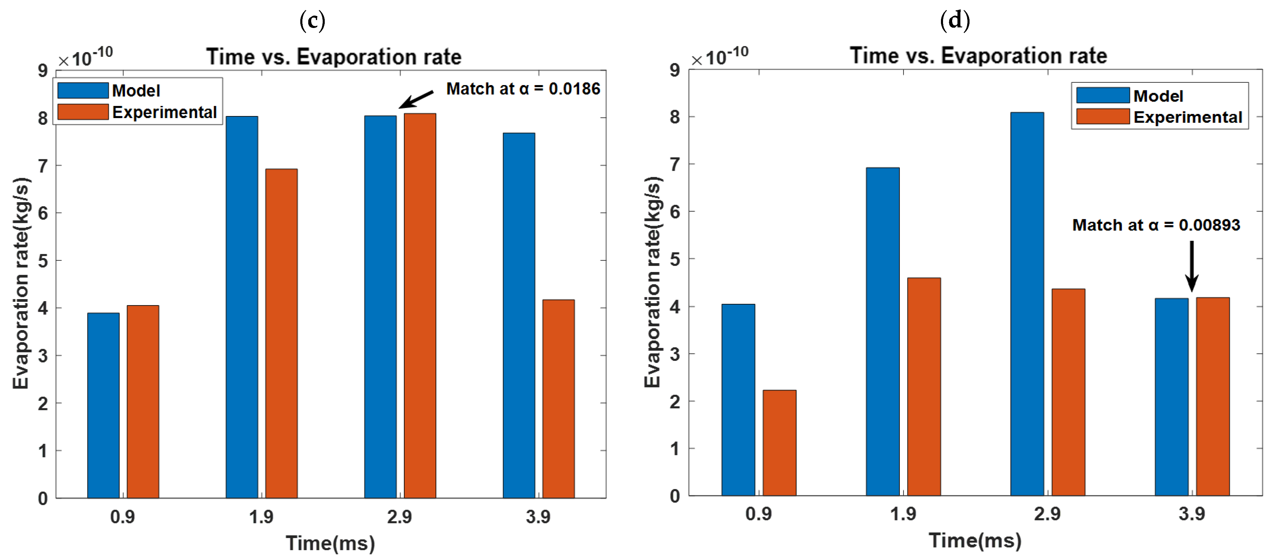
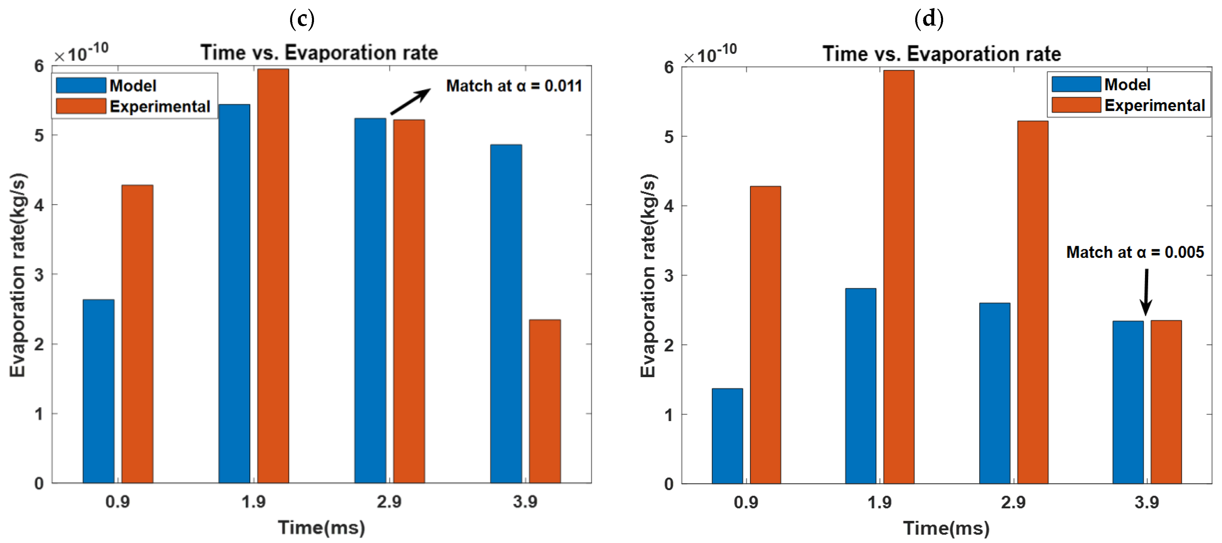
4.6. Effect of Accommodation Coefficient

This section explores the sensitivity of results by changing the value of the accommodation coefficient. Many studies used unity for the accommodation coefficient, which indicates a perfect evaporation capacity. This means that, for every liquid molecule released, none are rebounded and reabsorbed [42]. Using unity for the accommodation coefficient might be unrealistic, and it is very difficult to have extreme vapor purity in an experimental setup. It should be noted that purity is one of many factors that can reduce the accommodation coefficient from its theoretical upper limit. However, varying the accommodation coefficient results in very minimal film thickness change, as shown in Figure 11a. The variations of interfacial temperature and evaporative mass flux are indicated in Figure 11b,c. With a decreasing accommodation coefficient, the peak magnitude of the evaporative mass flux decreases, and the corresponding interfacial temperature indicates a higher temperature at the thickest region. The peak of evaporative mass flux is highly dependent on the coefficient value used. These results indicate that using different accommodation coefficients has a significant impact on the thin film’s evaporative properties.

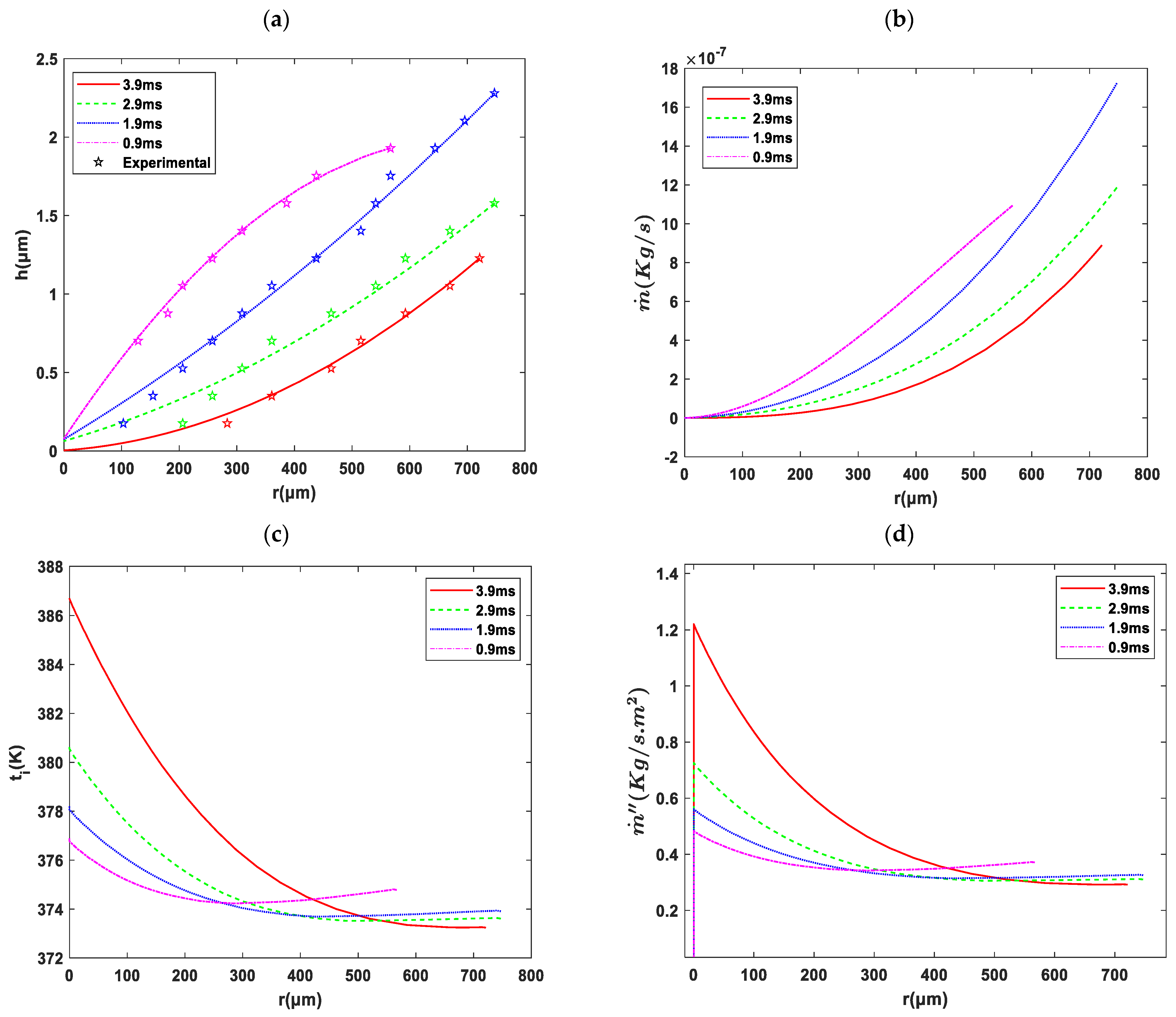
4.7. Effect of Time Step

All the results discussed in the previous sections are illustrated at a snapshot in time (time step 3.9 ms). However, experimental data was obtained at 1 ms intervals and comparisons can be made at each time step. This section expands the previous discussion for multiple time steps. The numerical model was run for different time steps at 0.9, 1.9, 2.9, and 3.9 ms with variable wall temperature, applied slip velocity, and an accommodation coefficient of 0.01. Initially, the variations of the wall temperature for different time steps are depicted and compared with the experimental results, which can be seen in Figure 3b. Wall temperature from the experimental data shows that initially, the wall temperature is highest in the thick region of the film. However, as time progresses, the wall temperature peak shifts to the thinner region of the film. When this is accounted for, the thin film profile from the model is in good agreement with the experimental results for all time steps. Changes in the film thickness, mass flow rate, interfacial temperature, and evaporative mass flux, are depicted in Figure 12a–d, respectively. As can be seen in Figure 12a, the radius of the bubble clearly increased at each region of the film by increasing the time step. Additionally, Figure 12b shows that, at a particular point of the bubble radius, a higher mass flow rate is observed for smaller time steps in the thicker region and obtained a near-zero flow rate at the thinnest region. The interfacial temperature shows an increase in peak magnitude as time increases (Figure 12c). Similarly, the mass flux peak at the thinnest region increases with time (Figure 12d).

4.8. Net Evaporation Rate of the Microlayer

The local mass flux distribution from the numerical model (Figure 11c) is integrated over the entire three-dimensional surface area of the bubble (based on Figure 11a) to obtain the total evaporation rate from the microlayer region. Mass fluxes are calculated from the experimentally measured wall, and evaporation heat fluxes across the microlayer using Equation (27) are also calculated based on Figure 3c:
m ˙ = q h f g
The mass flux obtained from both the model (Figure 12d) and the experiments (Figure 3c) could be integrated over the film profile (Figure 12a) to obtain an overall evaporation rate. The accommodation coefficient can then be varied to match the evaporation rates from both the model and the experiment. Figure 13 shows the comparison between the net evaporation rate from the model and the experimental wall heat flux derived evaporation rate at various time steps. Figure 13a shows that the time step of 0.9 ms, in conjunction with an accommodation coefficient value of 0.0198, results in a match between numerical and experimental results of the net evaporation rates. However, the same coefficient results in a systemic underprediction of the modeled rate at higher time steps, as seen in Figure 13a. Similar trends are seen at 0.9 ms, 1.9 ms, 2.9, and 3.9 ms, where accommodation coefficients of 0.019, 0.015, 0.0186, and 0.00893 match the experimentally derived wall heat flux data. These results suggest that the accommodation coefficient may not be a constant and is likely time dependent. The rates derived from the evaporation heat flux (Figure 3c) were also compared to the model. Similarly, as seen in Figure 14, the comparison between the experimental evaporation heat flux and the net evaporation rate from the model derived evaporation rate at various time steps, which represented different matching values of the accommodation coefficient. Figure 14a–d indicate that the accommodation coefficients of the experimental data (evaporation heat flux) and numerical model are matched at 0.0214, 0.0124, 0.011, and 0.005 at time steps of 0.9, 1.9, 2.9, and 3.9, respectively. Based on the results in Figure 13 and Figure 14, the matching accommodation coefficients decrease with time, suggesting that the accommodation coefficient may not be a constant. This observation was also recently made by Tecchio [43], where “interfacial resistance” increased with time as the microlayer was formed. An increase in the interfacial resistance is analogous to a decrease in the value of the accommodation coefficient, as both effects reduce the overall evaporation flux. The accumulation of impurities at the interface between the liquid and vapor as the bubble grows could explain this reduction [43] and is the likely reason for the systemic decrease in the accommodation coefficient observed here.
Giustini et al. [35], and Bures and Sato [44] also estimated the accommodation coefficient from the microlayer to be 0.03 and 0.034, respectively. These values are higher than the ones reported here, and the discrepancy is because we allow for both a variable wall and interfacial temperature while Giustini et al. [35] used a constant wall temperature and Bures and Sato [44] assumed isothermal interface temperature. This suggests that assuming an isothermal condition, either at the wall or at the interface, has the potential to overestimate the coefficient in the microlayer. Finally, the fact that all of the values here are much less than unity suggests that only a fraction of impinging vapor molecules is absorbed by a liquid surface and that there is a high possibility of molecular reflection at the liquid–vapor interface.

5. Conclusions

Understanding the microlayer is critical to advancement in nucleate boiling since it is a major contributor to the phase change heat transfer. However, thin film evolution, spatio-temporal stability, and the impact on macroscale bubble dynamics are still poorly understood. Using a lubrication theory approach that accounts for mass, momentum, and energy balances, a film evolution equation is developed. The interfacial mass transfer is modeled using kinetic theory where the accommodation coefficient is a necessary input. While most prior models begin the solution at the nanoscale adsorbed film, the current study reverses the integration path. Contrary to most prior models, the current formulation uses a variable wall temperature boundary rather than a constant wall temperature boundary. Experimentally determined film thickness derivatives are used as boundary conditions at the thicker end of the film, and the model is solved till an absorbed film is obtained. The model is validated by comparing the film thickness with experimental results. The phase change flux was integrated over the film to obtain a net rate. By comparing the net phase change flux from the model with the independently measured experimental values, the accommodation coefficient was estimated for various time steps. Key findings are summarized below:
  • Starting with experimentally measurable initial conditions in the bulk region removes the need to guess or tune boundary conditions at the adsorbed film, as performed in prior studies. Consequently, the film thickness and derivatives in the adsorbed film become outputs of the model rather than guessed inputs.
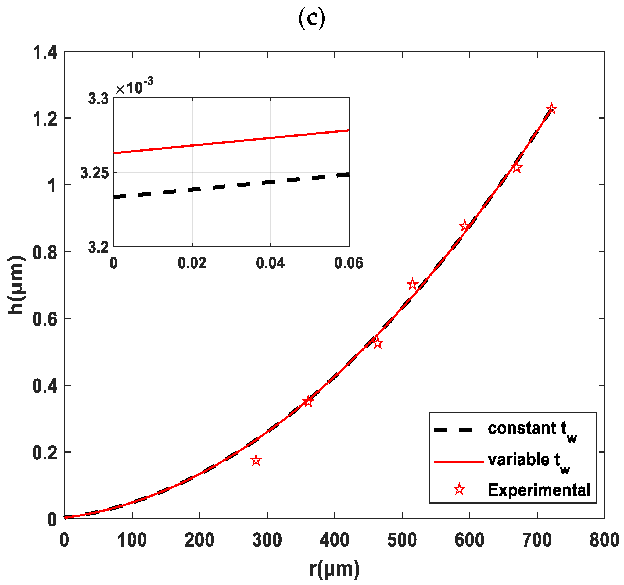
  • A constant wall temperature boundary suppresses the evaporation non-uniformity and shifts the mass flux profiles toward the thicker film. On the other hand, a variable wall temperature allows for a sharper peak in evaporation flux in the thin film vicinity.
  • Applying the slip velocity condition in the model led to a higher mass flow rate, allowing more bulk liquid flow under the bubble compared to a no slip boundary.
  • The value of the accommodation coefficient affects the peak magnitude of evaporative mass flux significantly. By comparing the experimentally measured spatiotemporally resolved heat flux measurements with the results from the model, the accommodation coefficient could be estimated. The results show that the accommodation coefficient most likely reduces with time as the microlayer evolves. It is likely that this systemic variation in the accommodation coefficient is due to either the accumulation of impurities [43] or an increase in surface interface temperature with time [45]. Future investigations on spatio-temporal variation in accommodation coefficient are recommended.

Author Contributions

Conceptualization, G.G. and H.K.; formal analysis, K.B. and E.L.; investigation, K.B., E.L. and G.G.; methodology, K.B.; supervision, K.B., G.G. and H.K.; visualization, E.L. and A.S.; writing—original draft, E.L. and A.S.; writing—review and editing, K.B., A.S., G.G. and H.K. All authors have read and agreed to the published version of the manuscript.

Funding

This research was partly funded by the United Kingdom Engineering and Physical Sciences Research Council (EPSRC) through grant EP/T027061/2 and the APC was funded by the University of Cincinnati through the Department of Mechanical and Materials Engineering.

Data Availability Statement

The data presented in this study are available on request from the corresponding author.

Acknowledgments

We acknowledge support from the University of Cincinnati in form of aGraduate Incentive Award for Ermiyas Lakew and a Graduate Assistant Scholarship for Amirhosein Sarchami.

Conflicts of Interest

The authors declare no conflict of interest.

Nomenclature

List of symbols
A Dispersion constant ( J ) u s Velocity of thin film ( m   s 1 )
C p Specific heat ( J   kg 1   K 1 ) V l Molar volume ( m 3   mol 1 )
d m Microlayer thickness ( m )Greek symbols
h Film thickness ( m ) α Accommodation coefficient (-)
h ,   h ,   h Film thickness derivatives (-) μ Dynamic viscosity ( kg   m 1   s 1 )
h f g Latent heat ( J   kg 1 ) ρ Mass density ( kg   m 3 )
K Surface curvature ( m 1 ) λ Wavelength ( m )
K b Boltzmann’s constant ( J   s 1   m 2   K 3 ) γ Slope of surface tension against temperature ( N   m 1   K 1 )
k Thermal conductivity ( W   m 1   K 1 ) σ Surface tension ( N   m 1 )
M Molar mass ( kg   mol 1 ) θ Refraction angle (°)
m ˙ Evaporation mass flux ( kg     s 1   m 2 )Subscripts
n l Refractive index (-)cCapillary
P Pressure ( Pa ) d Disjoining
q Heat flux () i Interfacial
r Radius ( m ) l Liquid
R ¯ Universal gas constant ( J   kg 1   K 1 ) v Vapor
T Temperature ( K ) w Wall

References

  1. Polansky, J. Numerical Model of an Evaporating Thin Film. Ph.D. Thesis, Carleton University, Ottawa, ON, Canada, 2011. [Google Scholar]
  2. Sodtke, C.; Kern, J.; Schweizer, N.; Stephan, P. High Resolution Measurements of Wall Temperature Distribution underneath a Single Vapour Bubble under Low Gravity Conditions. Int. J. Heat Mass Transf. 2006, 49, 1100–1106. [Google Scholar] [CrossRef]
  3. Hu, C.; Pei, Z.; Shi, L.; Tang, D.; Bai, M. Phase Transition Properties of Thin Liquid Films with Various Thickness on Different Wettability Surfaces. Int. Commun. Heat Mass Transf. 2022, 135, 106125. [Google Scholar] [CrossRef]
  4. Matin, M.H.; Moghaddam, S. Thin Liquid Films Formation and Evaporation Mechanisms around Elongated Bubbles in Rectangular Cross-Section Microchannels. Int. J. Heat Mass Transf. 2020, 163, 120474. [Google Scholar] [CrossRef]
  5. Ahmed, S.; Pandey, M. New Insights on Modeling of Evaporation Phenomena in Thin Films. Phys. Fluids 2019, 31, 092001. [Google Scholar] [CrossRef]
  6. Akkuş, Y.; Dursunkaya, Z. A New Approach to Thin Film Evaporation Modeling. Int. J. Heat Mass Transf. 2016, 101, 742–748. [Google Scholar] [CrossRef]
  7. Dwivedi, R.; Pati, S.; Singh, P.K. Combined Effects of Wall Slip and Nanofluid on Interfacial Transport from a Thin-Film Evaporating Meniscus in a Microfluidic Channel. Microfluid. Nanofluid. 2020, 24, 84. [Google Scholar] [CrossRef]
  8. Wang, H.; Pan, Z.; Chen, Z. Thin-Liquid-Film Evaporation at Contact Line. Front. Energy Power Eng. China 2009, 3, 141–151. [Google Scholar] [CrossRef]
  9. Zheng, Z.; Zhou, L.; Du, X.; Yang, Y. Numerical Investigation on Conjugate Heat Transfer of Evaporating Thin Film in a Sessile Droplet. Int. J. Heat Mass Transf. 2016, 101, 10–19. [Google Scholar] [CrossRef]
  10. Wee, S.-K.; Kihm, K.D.; Hallinan, K.P. Effects of the Liquid Polarity and the Wall Slip on the Heat and Mass Transport Characteristics of the Micro-Scale Evaporating Transition Film. Int. J. Heat Mass Transf. 2005, 48, 265–278. [Google Scholar] [CrossRef]
  11. Bellur, K.; Médici, E.F.; Choi, C.K.; Hermanson, J.C.; Allen, J.S. Multiscale Approach to Model Steady Meniscus Evaporation in a Wetting Fluid. Phys. Rev. Fluids 2020, 5, 024001. [Google Scholar] [CrossRef]
  12. Ball, G. Numerical Analysis of the Heat Transfer Characteristics within an Evaporating Meniscus. Ph.D. Thesis, Carleton University, Ottawa, ON, Canada, 2012. [Google Scholar]
  13. Kou, Z.-H.; Lv, H.-T.; Zeng, W.; Bai, M.-L.; Lv, J.-Z. Comparison of Different Analytical Models for Heat and Mass Transfer Characteristics of an Evaporating Meniscus in a Micro-Channel. Int. Commun. Heat Mass Transf. 2015, 63, 49–53. [Google Scholar] [CrossRef]
  14. Park, K.; Lee, K.-S. Flow and Heat Transfer Characteristics of the Evaporating Extended Meniscus in a Micro-Capillary Channel. Int. J. Heat Mass Transf. 2003, 46, 4587–4594. [Google Scholar] [CrossRef]
  15. Park, K.; Noh, K.-J.; Lee, K.-S. Transport Phenomena in the Thin-Film Region of a Micro-Channel. Int. J. Heat Mass Transf. 2003, 46, 2381–2388. [Google Scholar] [CrossRef]
  16. Wayner, P.C., Jr.; Kao, Y.K.; LaCroix, L.V. The Interline Heat-Transfer Coefficient of an Evaporating Wetting Film. Int. J. Heat Mass Transf. 1976, 19, 487–492. [Google Scholar] [CrossRef]
  17. Wayner, P.C., Jr. Intermolecular Forces in Phase-Change Heat Transfer: 1998 Kern Award Review. AIChE J. 1999, 45, 2055–2068. [Google Scholar] [CrossRef]
  18. Chatterjee, A.; Plawsky, J.L.; Wayner, P.C., Jr. Disjoining Pressure and Capillarity in the Constrained Vapor Bubble Heat Transfer System. Adv. Colloid Interface Sci. 2011, 168, 40–49. [Google Scholar] [CrossRef]
  19. Khurshid, I.; Al-Shalabi, E.W. New Insights into Modeling Disjoining Pressure and Wettability Alteration by Engineered Water: Surface Complexation Based Rock Composition Study. J. Pet. Sci. Eng. 2022, 208, 109584. [Google Scholar] [CrossRef]
  20. Do, K.H.; Kim, S.J.; Garimella, S.V. A Mathematical Model for Analyzing the Thermal Characteristics of a Flat Micro Heat Pipe with a Grooved Wick. Int. J. Heat Mass Transf. 2008, 51, 4637–4650. [Google Scholar] [CrossRef] [Green Version]
  21. Zhao, J.-J.; Duan, Y.-Y.; Wang, X.-D.; Wang, B.-X. Effects of Superheat and Temperature-Dependent Thermophysical Properties on Evaporating Thin Liquid Films in Microchannels. Int. J. Heat Mass Transf. 2011, 54, 1259–1267. [Google Scholar] [CrossRef]
  22. Azarkish, H.; Behzadmehr, A.; Frechette, L.G.; Sheikholeslami, T.F.; Sarvari, S.M.H. A Modified Disjoining Pressure Model for Thin Film Evaporation of Water. In Proceedings of the ASME International Mechanical Engineering Congress and Exposition, San Diego, CA, USA, 15–21 November 2013; American Society of Mechanical Engineers: New York, NY, USA; Volume 56321, p. V07BT08A007. [Google Scholar]
  23. Holm, F.W.; Goplen, S.P. Heat Transfer in the Meniscus Thin-Film Transition Region. J. Heat Transf. 1979, 101, 543–547. [Google Scholar] [CrossRef]
  24. Wayner, P.C., Jr. The Effect of Interfacial Mass Transport on Flow in Thin Liquid Films. Colloids Surf. 1991, 52, 71–84. [Google Scholar] [CrossRef]
  25. Akkus, Y.; Gurer, A.T.; Bellur, K. Drifting Mass Accommodation Coefficients: In Situ Measurements from a Steady State Molecular Dynamics Setup. Nanoscale Microscale Thermophys. Eng. 2021, 25, 25–45. [Google Scholar] [CrossRef]
  26. Bellur, K.S. A New Technique to Determine Accommodation Coefficients of Cryogenic Propellants. Ph.D. Thesis, Michigan Technological University, Houghton, MI, USA, 2018. [Google Scholar]
  27. Carey, V.P. Liquid-Vapor Phase-Change Phenomena: An Introduction to the Thermophysics of Vaporization and Condensation Processes in Heat Transfer Equipment; CRC Press: Boca Raton, FL, USA, 2020. [Google Scholar]
  28. Hertz, H. Ueber die Verdunstung der Flüssigkeiten, Insbesondere des Quecksilbers, im Luftleeren Raume. Ann. Phys. 1882, 253, 177–193. [Google Scholar] [CrossRef] [Green Version]
  29. Knudsen, M. The Kinetic Theory of Gases: Some Modern Aspects; Methuen & Company Limited: London, UK, 1934. [Google Scholar]
  30. Marek, R.; Straub, J. Analysis of the Evaporation Coefficient and the Condensation Coefficient of Water. Int. J. Heat Mass Transf. 2001, 44, 39–53. [Google Scholar] [CrossRef]
  31. Schrage, R.W. A Theoretical Study of Interphase Mass Transfer. In A Theoretical Study of Interphase Mass Transfer; Columbia University Press: New York, NY, USA, 1953. [Google Scholar]
  32. Bellur, K.; Médici, E.F.; Kulshreshtha, M.; Konduru, V.; Tyrewala, D.; Tamilarasan, A.; McQuillen, J.; Leão, J.B.; Hussey, D.S.; Jacobson, D.L. A New Experiment for Investigating Evaporation and Condensation of Cryogenic Propellants. Cryogenics 2016, 74, 131–137. [Google Scholar] [CrossRef] [Green Version]
  33. Jung, S.; Kim, H. An Experimental Method to Simultaneously Measure the Dynamics and Heat Transfer Associated with a Single Bubble during Nucleate Boiling on a Horizontal Surface. Int. J. Heat Mass Transf. 2014, 73, 365–375. [Google Scholar] [CrossRef]
  34. Jung, S.; Kim, H. An Experimental Study on Heat Transfer Mechanisms in the Microlayer Using Integrated Total Reflection, Laser Interferometry and Infrared Thermometry Technique. Heat Transf. Eng. 2015, 36, 1002–1012. [Google Scholar] [CrossRef]
  35. Giustini, G.; Jung, S.; Kim, H.; Ardron, K.H.; Walker, S.P. Microlayer Evaporation during Steam Bubble Growth. Int. J. Therm. Sci. 2019, 137, 45–54. [Google Scholar] [CrossRef]
  36. DasGupta, S.; Schonberg, J.A.; Wayner, P.C., Jr. Investigation of an Evaporating Extended Meniscus Based on the Augmented Young–Laplace Equation. J. Heat Transf. 1993, 115, 201–208. [Google Scholar] [CrossRef]
  37. Adamson, A.W.; Gast, A.P. Physical Chemistry of Surfaces; Interscience Publishers: New York, NY, USA, 1967; Volume 150. [Google Scholar]
  38. Li, J.; Yang, Z.; Duan, Y. Numerical Simulation of Single Bubble Growth and Heat Transfer Considering Multi-Parameter Influ-ence during Nucleate Pool Boiling of Water. AIP Adv. 2021, 11, 125207. [Google Scholar] [CrossRef]
  39. Liu, Y.; Xing, Y.; Yang, C.; Li, C.; Xue, C. Simulation of Heat Transfer in the Progress of Precision Glass Molding with a Finite Element Method for Chalcogenide Glass. Appl. Opt. 2019, 58, 7311–7318. [Google Scholar] [CrossRef] [PubMed]
  40. Du, S.-Y.; Zhao, Y.-H. Numerical Study of Conjugated Heat Transfer in Evaporating Thin-Films near the Contact Line. Int. J. Heat Mass Transf. 2012, 55, 61–68. [Google Scholar] [CrossRef]
  41. Emelyanenko, K.A.; Emelyanenko, A.M.; Boinovich, L.B. Disjoining Pressure Analysis of the Lubricant Nanofilm Stability of Liquid-Infused Surface upon Lubricant Depletion. J. Colloid Interface Sci. 2022, 618, 121–128. [Google Scholar] [CrossRef]
  42. Kaya, T.; Ball, G.; Polansky, J. Investigation of Particular Features of the Numerical Solution of an Evaporating Thin Film in a Channel. Front. Heat Mass Transf. 2013, 4, 013002. [Google Scholar] [CrossRef] [Green Version]
  43. Tecchio, C. Experimental Study of Boiling: Characterization of Near-Wall Phenomena and Bubble Dynamics. Ph.D. Thesis, Université Paris-Saclay, Paris, France, 2022. [Google Scholar]
  44. Bureš, L.; Sato, Y. Comprehensive Simulations of Boiling with a Resolved Microlayer: Validation and Sensitivity Study. J. Fluid Mech. 2022, 933, A54. [Google Scholar] [CrossRef]
  45. Nagayama, G.; Takematsu, M.; Mizuguchi, H.; Tsuruta, T. Molecular Dynamics Study on Condensation/Evaporation Coefficients of Chain Molecules at Liquid–Vapor Interface. J. Chem. Phys. 2015, 143, 014706. [Google Scholar] [CrossRef] [Green Version]
Figure 1. Schematic of an evaporating extended meniscus in the “microlayer” region.
Fluids 08 00126 g001
Figure 2. (a) Schematic diagram of the experimental setup; (b) Example image of interferometric pattern from bubble total reflection [33,34].
Fluids 08 00126 g002
Figure 3. Radius evolutions of microlayer film thickness (a), variable wall temperature (b), and calculations of heat flux using two different methods (c). The black arrow in Figure 3a shows the temporal displacement for a constant film thickness. For brevity, heat flux data at only 3.9 ms is shown here. Please refer to [33,34,35] for additional details.
Fluids 08 00126 g003
Figure 4. Solution setup used to solve the interfacial temperature and evaporative mass flux in the thin film.
Fluids 08 00126 g004
Figure 5. Comparison of the numerical model and experimental results based on film thickness at a time step of 3.9 ms [33,34].
Fluids 08 00126 g005
Figure 6. Radius evolutions of (a) disjoining pressure; (b) mass flow rate; (c) interfacial temperature; and (d) evaporation mass flux for baseline parameters at a time step of 3.9 ms.
Fluids 08 00126 g006aFluids 08 00126 g006b
Figure 7. Radius evolutions of (a) interfacial temperature; (b) evaporative mass flux; and (c) film thickness for different conditions at a time step of 3.9 ms.
Fluids 08 00126 g007aFluids 08 00126 g007b
Figure 8. Radius evolutions of (a) evaporative mass flux; and (b) film thickness for no slip and slip conditions at a time step of 3.9 ms.
Fluids 08 00126 g008
Figure 9. Radius evolutions of (a) disjoining pressure; (b) mass flow rate; (c) film thickness; and (d) evaporative mass flux for different disjoining pressure models at a time step of 3.9 ms.
Fluids 08 00126 g009
Figure 10. Radius evolutions of (a) disjoining pressure; and (b) evaporative mass flux for different dispersion constants at a time step of 3.9 ms.
Fluids 08 00126 g010
Figure 11. Radius evolutions of (a) film thickness; (b) interfacial temperature; and (c) evaporative mass flux for different accommodation coefficients at a time step of 3.9 ms.
Fluids 08 00126 g011
Figure 12. Radius evolutions of (a) film thickness; (b) mass flow rate; (c) interfacial temperature; and (d) evaporative mass flux for different time steps.
Fluids 08 00126 g012
Figure 13. A comparison between the evaporation rates of the model and experimentally derived wall heat flux at various times of 0.9 ms (a), 1.9 ms (b), 2.9 ms (c), and 3.9 ms (d). The accommodation coefficient could be estimated through iterative matching. The results suggest that the matched coefficient reduces with time.
Fluids 08 00126 g013aFluids 08 00126 g013b
Figure 14. A comparison between evaporation rates between the model and experimentally derived evaporation heat flux at various times of 0.9 ms (a), 1.9 ms (b), 2.9 ms (c), and 3.9 ms (d). The accommodation coefficient could be estimated through iterative matching. The results suggest that the matched coefficient reduces with time.
Fluids 08 00126 g014aFluids 08 00126 g014b
Table 1. Summary of prior and current approaches of modeling evaporation at the thin film.
StudyCoordinate SystemRadii of CurvatureWall Boundary ConditionStart of Integration Accommodation Coefficient
Akkuş and Dursunkaya, 2016 [6]Cartesian1ConstantBulk1
Wang et al., 2009 [8]Cartesian1ConstantAdsorbed1
Ahmed and Pandey, 2019 [5]Cartesian1ConstantAdsorbed1
Dwivedi et al., 2020 [7]Cartesian1ConstantAdsorbed1
Wee et al., 2005 [10]Cylindrical2ConstantAdsorbed1
Zheng et al., 2016 [9]Cartesian1ConstantAdsorbed1
Current studyCylindrical2VariableBulkEstimated
Disclaimer/Publisher’s Note: The statements, opinions and data contained in all publications are solely those of the individual author(s) and contributor(s) and not of MDPI and/or the editor(s). MDPI and/or the editor(s) disclaim responsibility for any injury to people or property resulting from any ideas, methods, instructions or products referred to in the content.

