

Fire Spread in Multi-Storey Timber Building, a CFD Study

Department of Mechanical and Product Design Engineering, Swinburne University of Technology, Hawthorn, VIC 3122, Australia
*
Author to whom correspondence should be addressed.
Fluids 2023, 8(5), 140; https://doi.org/10.3390/fluids8050140
Submission received: 12 March 2023
/
Revised: 19 April 2023
/
Accepted: 25 April 2023
/
Published: 28 April 2023
(This article belongs to the Special Issue Analytical and Computational Fluid Dynamics of Combustion and Fires [Dedicated to Prof. Vitaly Bychkov (1968–2015) of Umea University, Sweden], Volume II)
Abstract
:The purpose of this paper is to investigate the fire performance in a multi-storey cross-laminated timber (CLT) structure by the computational fluid dynamics (CFD) technique using the Fire Dynamics Simulator (FDS v.6.7). The study investigates fire temperature, heat release rate (HRR), and gas concentration (, ). The importance of this research is to ensure that the fire performance of timber buildings is adequate for occupant safety and property protection. Moreover, the proposed technique provides safety measures in advance for engineers when designing buildings with sufficient fire protection by predicting the fire temperature, time to flashover and fire behaviour. The present numerical modelling is designed to represent a 10-storey CLT residential building where each floor has an apartment with 9.14 m length by 9.14 width dimensions. The pyrolysis model was performed with thermal and kinetic parameters where the furniture, wood cribs and CLT were allowed to burn by themselves in simulation. This research is based on a full-scale experiment of a two-storey CLT building. The present results were validated by comparing them with the experimental data. Numerical simulation of CLT building models show a very close accuracy to the experiment performed in the benchmark paper. The results show that the CFD tools such as FDS can be used for predicting fire scenarios in multi-storey CLT buildings.
1. Introduction
Nowadays, there is a trend towards multi-storey cross-laminated timber (CLT) buildings. Due to this trend, the research needs to evolve a comparison between traditional concrete buildings and CLT buildings. Fires and smoke in multi-floor buildings are well known threats to individuals and property. Use of CLT as a structural element in mid- and high-rise buildings is limited owing to its combustible nature. Many multi-storey timber buildings have been constructed, and most of them have not complied with fire safety or have very little data about fire performance [1]. The fire performance of the CLT structural building can be accurately modelled by performing full-scale fire experimental or numerical simulation using CFD tools. However, a full-scale test on high-rise CLT buildings was never performed to obtain complete information about fire spread, heat temperature or heat release rate. Furthermore, fire and smoke models for CLT buildings are very limited compared to a traditional concrete building.
Understanding the modelling of the fire performance of multi-storey CLT buildings is necessary to ensure the fire resistance capacity of timber structures is adequate for occupant safety and property protection. This also assists engineers in designing buildings with sufficient fire protection by predicting the fire temperature, time to flashover, passive fire resistance and fire behaviour inside and outside the building.
During the recent few decades, more than 70% of people around the world have lived in timber structure houses [2]. CLT is a large-scale modern engineering wood product that involves multiple layers of lumber boards [3]; the characteristics of CLT such as rigidity and strength, allow it to be used in high- and mid-rise buildings. Several tall timber buildings have been constructed globally, such as the 14-storey Treet building in Bergen, Norway, opened in 2015 [4], the 10-storey 25 King building in Brisbane, Australia opened in 2016 [5] and the 10-storey Forte Docklands building in Melbourne, Australia opened in 2013 [6]. Currently, the Tallest Timber building tower is Under Construction in Sydney, Australia, which will be 40-storey once complete in 2025 [7].
Many experiments have been carried out on CLT structures to investigate and evaluate fire performance. Su et al. (2018) [8] performed full series experiments for full-scale rooms encapsulated using mass timber construction to provide further understanding of the fire behaviour of mass timber elements. Emberley et al. (2017) [9] conducted small and large-scale fire tests on CLT compartment fires; the internal walls were protected by non-combustible board except one wall which was exposed to fire. Wood cribs were used as fuel load. Heat flux, gas flow velocities and gas temperature were measured. Hoehler et al. (2018) [10] investigated the contribution of CLT building elements in compartment fires, where six large-scale fire tests were conducted. The residential contents, CLT structural panels and furniture, were used to obtain 550 MJ/m2 of fuel. The gypsum board was used to cover CLT exposed surfaces. The experiment’s results demonstrated that the exposed surface of CLT and ventilation condition played a crucial effect in the experimental data results, and that the gypsum board was capable of preventing or delaying CLT’s participation in the fire. As a result of the experimental study demonstrating that it was possible to minimise the delamination due to fire, it recommended the use of heat resistant adhesives in CLT. Gorska et al. (2021) [11] carried out experiments to obtain data concerning mass timber compartments by study the burning behaviour of timber, flow fields and gas phase temperatures.
Despite the lack of numerical simulation studies using CFD of mid- and high-rise CLT buildings, there are many fire studies of traditional concrete buildings using CFD. Fernandes et al. (2021) [12] studied the radiative heat transfer in fire using FDS for an open and a closed compartment. The liquid fuels for each model were methanol, heptane and ethanol. Betting et al. (2019) [13] used FDS to validate the experimental study of smoke dynamics in a compartment fire. Long-fei et al. (2011) [14] carried out numerical simulation of high-rise buildings to analyse the spread of fire and temperature distribution. Yi et al. (2019) [15] used FDS to simulate fire flame spread outcomes in buildings. Good prediction results were also achieved with FDS for simulation of fire spread characteristics in several types of overcrowded buildings such as supermarkets [16], hospitals [17], offices [18] and theatres [19]. The CFD study of fire in CLT buildings is almost non-existent in open literature.
The present research was conducted to study the performance of high-rise CLT buildings under fire. The numerical simulation was performed to predict the fire spread in a 10-storey CLT building. The numerical simulation focused on the air temperatures inside and outside the building, gas concentrations and HHR prediction of furniture and wood cribs. The built-in pyrolysis model in FDS v6.7 was used, incorporating thermal and kinetic parameters. The furniture and wood cribs were allowed to ignite by themselves in simulation. The research aims at assessing the fire safety of CLT building. The present research methodology and simulation data may provide a good benchmark for fire engineers and future fire modelling research on timber buildings.
In this work, CFD investigation was performed using Fire Dynamics Simulator (FDS v.6.7), which was developed by NIST [20]. FDS solves Navier–Stokes equations and governing equations of combustion materials [20,21]. The software simulates fire distribution and smoke propagation in buildings [22]. Turbulent fluid flow behaviour is included by adopting Large Eddy Simulation (LES). The FDS modelling allows access to real time data and reliable information that would help control all the factors present in a real-world fire situation.
2. Building Description and Simulation Details
2.1. Selected Experiment
Five full-scale fire experiments were carried out to investigate the performance of a two-storey CLT residential building. The experimental setup has been described in full detail in Zelinka et al. (2018) [23]. These experiments [23] were taken as reference to validate the present model. The original study of Zelinka et al. (2018) [23] conducted a detailed experiment of five full-scale compartment fire tests with a principle of oxygen consumption calorimetry on a two-story CLT building. The experiment examined the effect of ceilings and exposed walls on a practical full-size apartment to understand the effect of CLT under fire situations. The experiment is conducted on a two-story apartment building with areas designated for a bedroom, utility–laundry room, living room, and a kitchen. A corridor exists along two sides of the apartment with one end opened to the laboratory space and the other end connecting to a stairwell. Each apartment is 9.14 m wide by 9.14 m deep by 2.74 m high. The stairwell is 2.44 m wide by 4.88 m deep. The L-shaped corridor is 1.52 m wide and 2.74 m high. Each test was performed under different fire scenarios for a period of time up to 240 min. The experiments represent fire in real residential apartment buildings. The total fuel load was 570 MJ/m2 comprising furniture and wood cribs. All dimensions and boundary conditions used in the present numerical model were taken from the reference experiment [23]. All results from the present numerical model were compared at the exact physical locations as in these experiments [23]. Thus, the simulation results of the present model were comprehensively validated by comparing them with the experimental data.
2.2. Description of Proposed Building
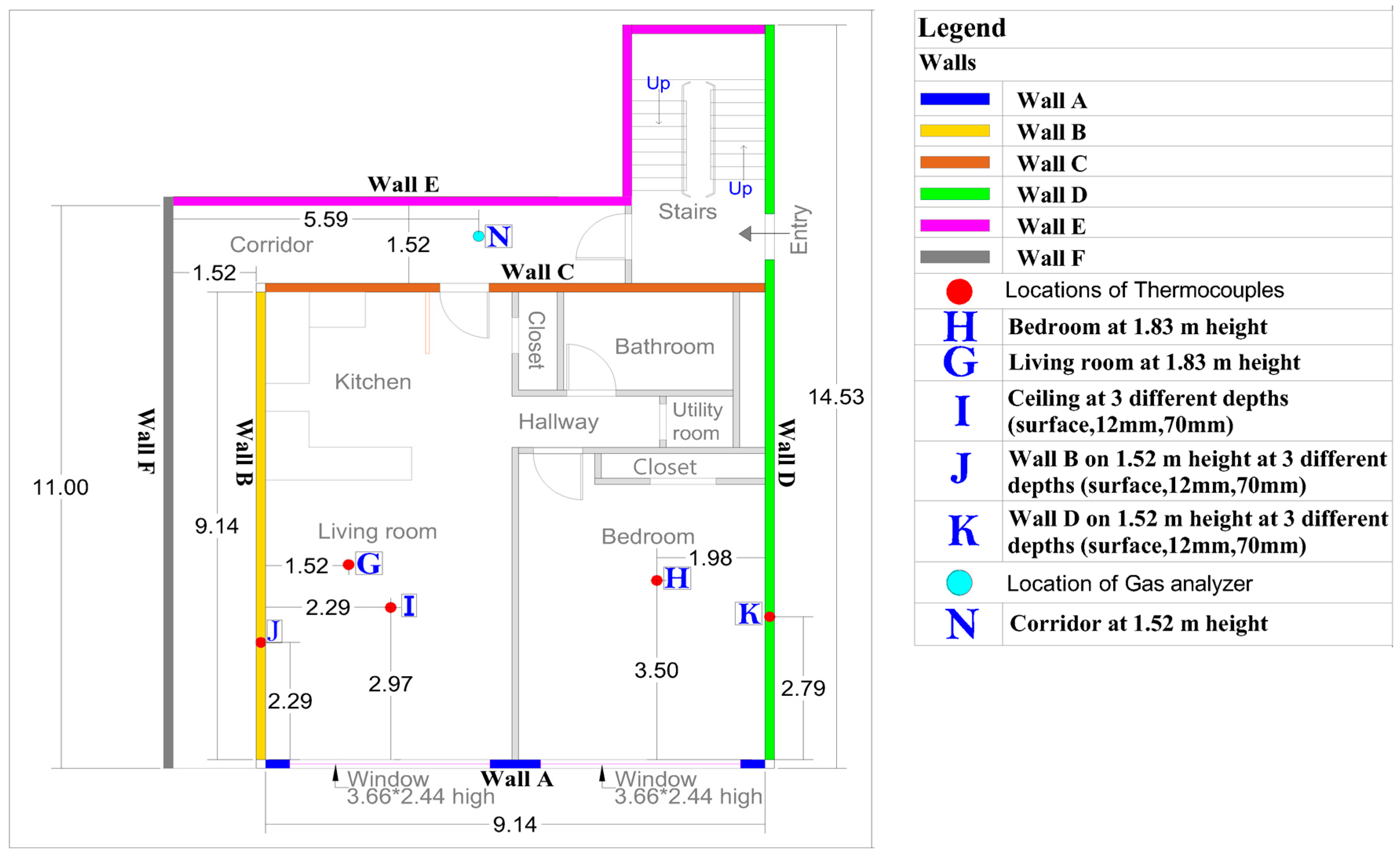
The proposed model is a 10-storey CLT building, Figure 1 illustrates the typical floor plan of the building layout with major details. The walls and locations of measurement instruments used inside the building are represented in the layout with letters (A, B, C, D, E, F, G, H, I, J, K, N), as shown in Figure 1. Each floor has an apartment of 9.14 m length by 9.14 m width and 2.75 m height. The corridor is 1.52 m in width and 2.75 m in height. The staircase is 2.44 m in width by 4.88 m in length. The total building height is 30 m. Each floor is divided into five-zone areas, including a living room, bedroom, open kitchen area, toilet and washing room.
The timber surfaces in the first two floors were encapsulated with gypsum wallboard, as per the reference experiments [23]. All stair doors and main apartment doors were kept closed during modelling, as per the reference experiments [23]. Windows on the first floor were kept open, and on the second floor were protected using gypsum wallboard (see Figure 2 and Figure 3b), as per the reference experiments [23]. Temperatures, heat release rate (HRR), and concentrations, and performance of the CLT building structure were evaluated.
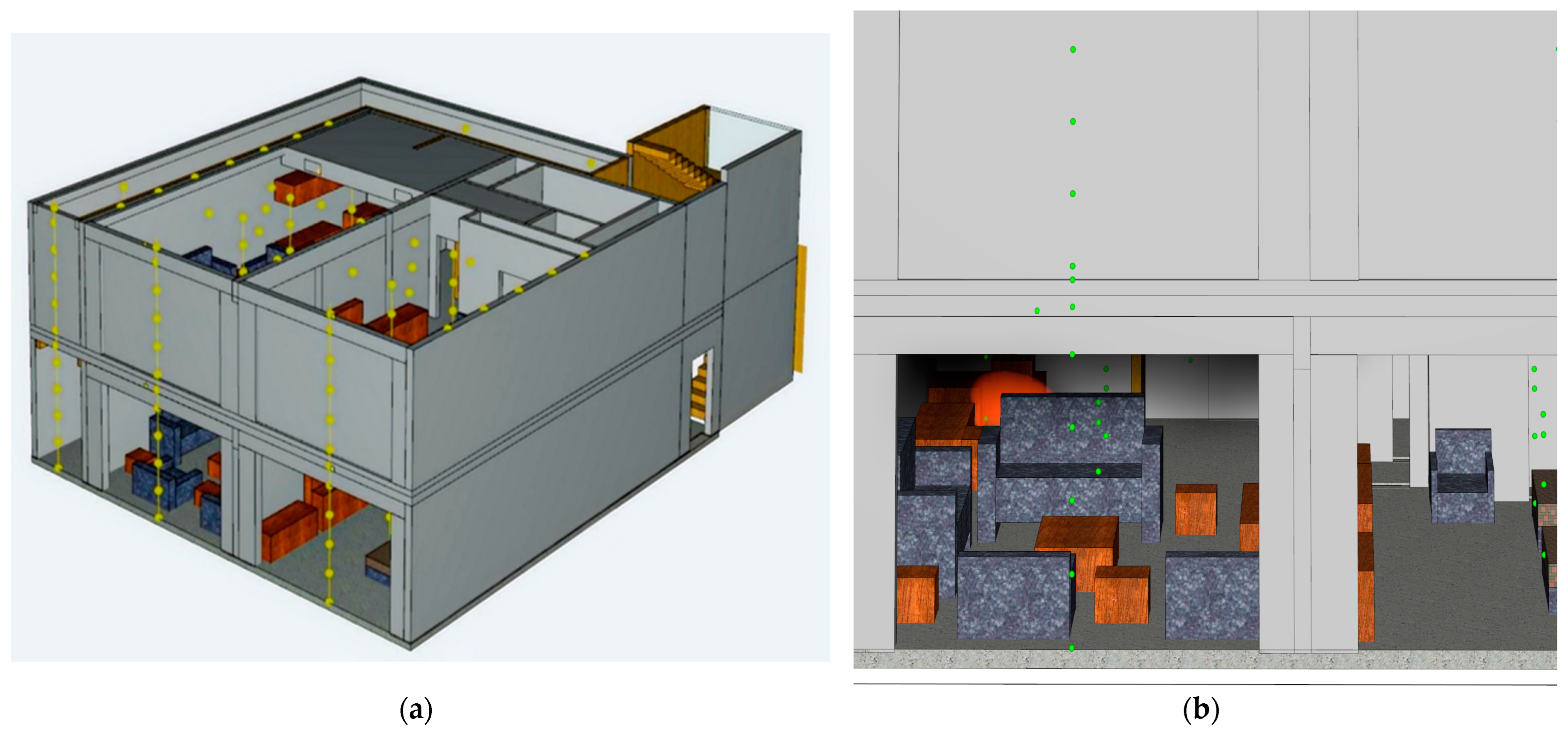
In the present simulation model, the locations of thermocouples were placed in the same positions as the reference experiments [23]. Figure 2a shows locations of thermocouples in yellow circle points, where 218 thermocouples were used along the proposed building in two configurations. 1. Multiple thermocouples were placed in a vertical layer 60 cm apart. 2. Single thermocouples were placed at various heights and locations along the building, as well as on the ceiling in each room on the first floor and second floor, as shown in Figure 2a.
According to experimental data [23], the fire scenario started on the first floor from the kitchen by ignition source of 250 mL of gasoline, as shown in Figure 2b. However, is the molecular formula of gasoline. The Thermal properties of gasoline were taken from [24] as explained in Table 1.
The complete combustion of hydrocarbons with oxygen will produce carbon dioxide and water vapour as follows:
Gas analysers were placed in the corridor on each floor to record and concentration. Estimation of HRR was based on the thermal property and heat release rate per unit area (HRRPUA) of combustible materials is explained in Section 3.
Multiple materials were used in the model. The properties of the materials used in the model were the same as in the reference experiment [23]. FDS uses the constant thermal properties for the surfaces of the solid materials. The details can be found in Hurley et al. (2015) [24]. Wood (yellow pine) was used in cribs to increase fuel load in the living room and bedroom. The proposed model was constructed from CLT consisting of beams, columns, walls, and ceiling. Concrete was used in the exterior surface of the CLT ceiling and on the floor of the first floor. Thus, the model was built directly on the concrete. Gypsum wallboards were used as interior walls between rooms in the apartment and to cover CLT (internal and external walls, ceiling, beams, and columns) as passive fire protection in the first two storeys, as shown in Figure 3b. The fire started in the corner of the kitchen (see Figure 2a), as was done in the reference experiment [23]. The total fuel load, including all furniture and the wood cribs throughout the apartment, was approximately 570 MJ/m2. The thermal properties of the furniture and construction materials used in the building were obtained from the literature [25,26,27]. The thermo-physical properties of the materials were taken as assumed in the literature of [25,26,27].
2.3. Computational Grid and Domain
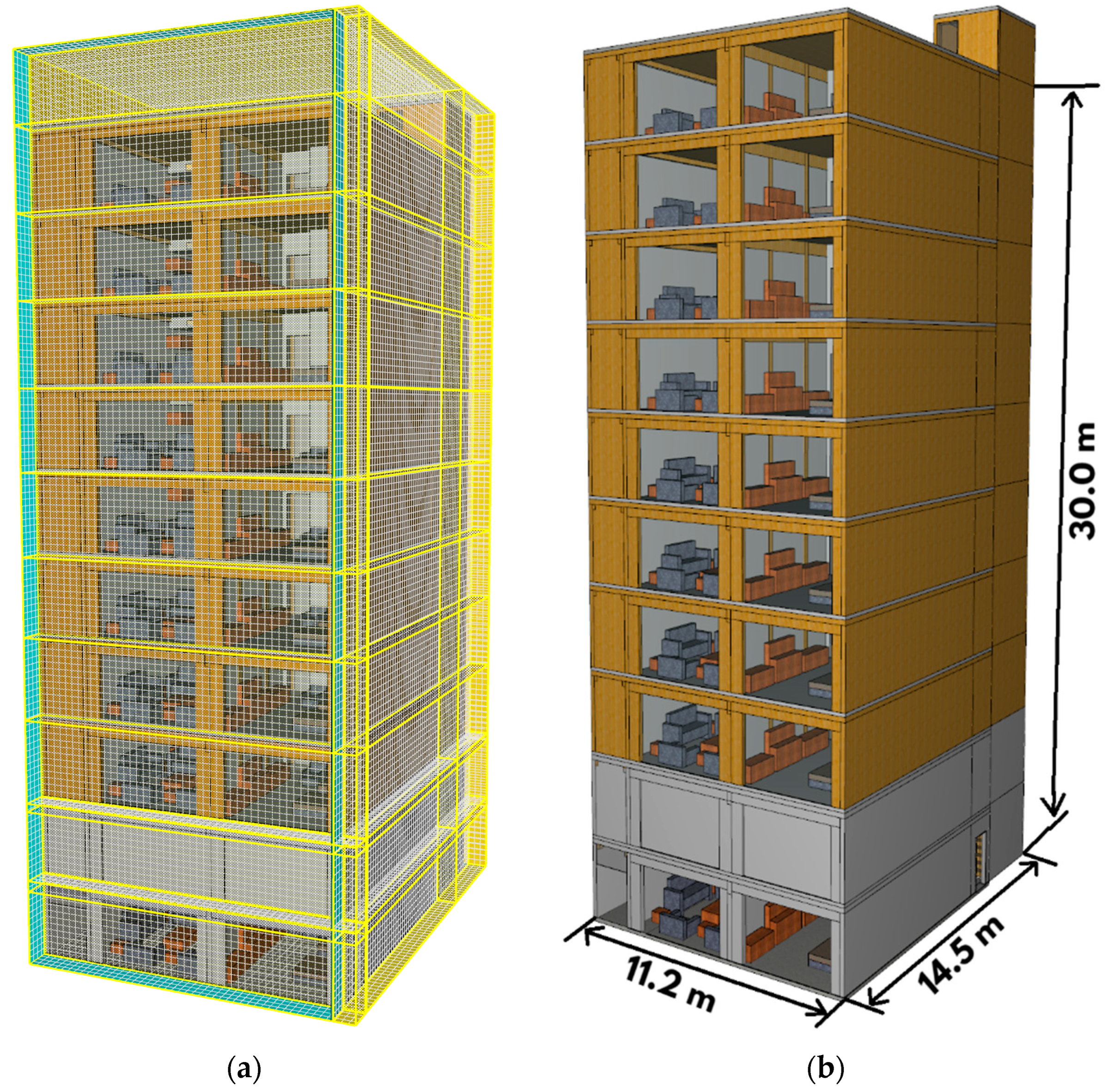
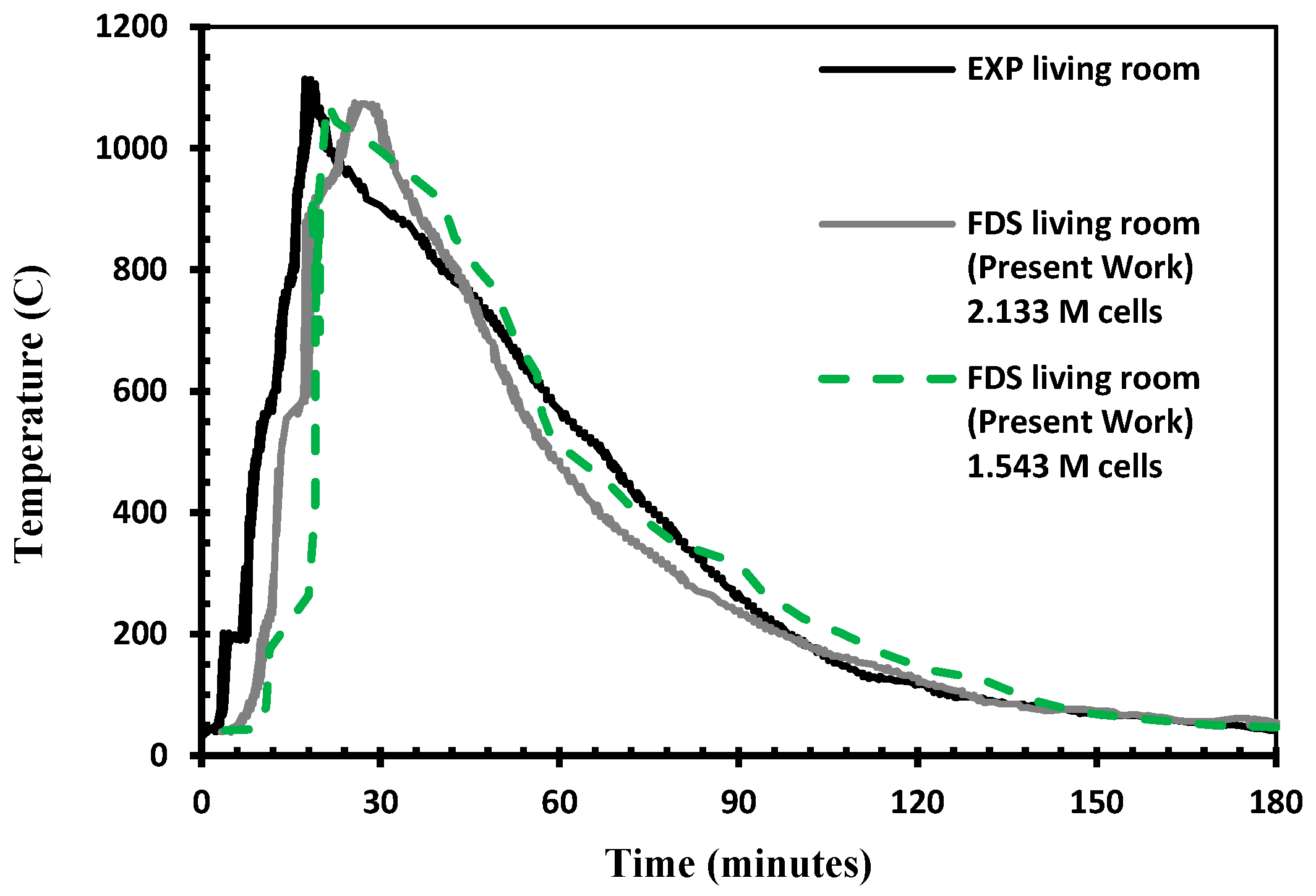
The dimensions of the CLT building model are 14.5 m, 11.2 m and 30 m (see Figure 3b). The building was divided into a computational grid. Grid independency tests were carried out. A total of 2,133,243 mesh (grid) cells were used, where every cubic cell dimension was (0.15 × 0.15 × 0.15 m). A sample of grid independency test, using 1,543,336 mesh cells (grid), is shown in Figure 4 and Figure 5. This grid independency test shows that a total of 2,133,243 mesh (grid) cells were good enough. This is also justified by the good agreement of results obtained with the 2,133,243 mesh cells against the experimental data. Figure 3a shows front view of the building with mesh blocks as used in the model. As can be seen, the computational mesh block is consistent throughout the simulation. The computational mesh resolution and distribution was varied until the impacts of computational mesh on simulated results were almost eliminated. Consequently, the present mesh structure can accurately capture the characteristics of thermal fields and flow. The numerical simulation was performed using the high-performance computing (HPC), supercomputing OzSTAR facility at Swinburne University which is providing computational resources to researchers.
The computational domain was extended around the building by 0.8 m on the right side, 1 m on the front side, 0.8 m above the roof of the tenth floor and 0.4 m on the rear side. These extensions were made to facilitate fire spreading out of the building through the windows on the first floor. Following the reference experiment [23], the external and internal wall thicknesses in the proposed model is 0.175 m and 0.127 m, respectively. The floor, walls, stairs and ceiling in the building model are made of CLT except for internal walls, which are made of gypsum, as per the reference experiment [23].
2.4. Boundary Conditions
At the start of numerical modelling (t = 0), the temperature and velocity of the indoor and outdoor regions of entire computation domain were assumed to be 20 °C and zero velocity, respectively. The total simulation time was 180 min. Using FDS code the numerical time-step is modified dynamically. Following the reference experiment [23], all boundary conditions were set accordingly. All stair doors and main apartment doors were kept closed during modelling. Windows on the first floor were kept open. As per the reference experiment, the door between the living room, the bedroom and the opening vent located in the front view on the first floor were kept open to remake a well-ventilated fire scenario. The fire scenario started on the first floor from the kitchen by igniting the fuel source of 250 mL gasoline, which is represented in the model as a rectangular volume with dimensions 1 m × 1 m and 0.2 m height.
The furniture and wood cribs were allowed to burn by themselves using pyrolysis model in FDS with proper thermal and kinetic parameters, where the pyrolysis of solid surfaces and fuel materials were assumed to be specified by setting HRRPUA for every surface material. All solid layers were designated the thermal boundary conditions and burning rate of materials. The heat release rate profile of the fire source in modelling was obtained from experimental report [23]. In the FDS model, the mass of wood is converted to 82% gaseous and 18% is converted to char.
3. Pyrolysis Model
Several fire models have been used [28] to study fire behaviour in building structures, where fire models range from simple models using maximum gas temperatures of a compartment fire to a complicated CFD model using software such as FDS v.6.7 [28]. Pyrolysis is carried out in FDS using appropriate material properties. FDS can handle both liquid and solid fuels [20]. Several layers of various materials can be assumed to exist on a solid surface. FDS assumes local thermal equilibrium between the volatiles and solids. FDS produces volatiles by converting appropriate amount solid fuels to gaseous phase under appropriate thermodynamic conditions.
The pyrolysis in FDS model is modelled using a finite rate reaction instead of the default mixing-controlled model. All gaseous species are identified, and the gaseous species produced from solid-phase reactions are defined.
The mass fraction of solid component α is calculated using the density of the solid component α, and density of composite material :
The densities of composite material is given by:
where is representing the number of solid material components. The general equation for a material that undergoes one or more reactions is:
where (in unit ) is the rate of consumption of component α. The second term on the right side in Equation (4) is the production rate ; it represents the sum of material components α, produced by reactions with a yield of .
The rate of reactions are a function of temperature and concentration of local mass, representing the amalgamation of power functions and Arrhenius through of the component material temperature (), and the rate of reactions including the optional term:
where is the optional threshold temperature, which allows definitions of ignition criteria and non-Arrhenius pyrolysis. A and E are parameters of the kinetic constants, as shown in Equations (7) and (8), respectively, and they can specify by the link temperature and rate .
If is equal to 1, in a simple pyrolysis model between a single reaction with a single component, is a heating rate (in unit ). Further details can be found in the FDS manual [20].
The rate of volumetric production for each gaseous volatile is calculated using the production rate , and initial density of the solid layer :
The gases were assumed to be transferred immediately to the surface material. The surface thickness (L) was used to calculate the mass fluxes:
The heat conduction equation of the reaction material presents in Equation (11), where is the term for a chemical source. The equation consists of the heat of combustion which provides the heat of reaction.
The evaporation rate of liquid fuel using the Clausius–Clapeyron equation is a function of the concentration of fuel vapour and the temperature of liquid above the combustible surface material form.
where is the volume fraction of volatile combustible gas above the fuel surface, which is a function of molecular weight (), heat of vaporisation ( and the liquid boiling temperature (. As a result, the mass flux of the vapour fuel above the surface, at the start of modelling was created first by the FDS user through specifying the initial vapour volume flux . However, in the modelling, the evaporation mass flux is updated by identifying the difference between the specified equilibrium value obtained from Equation (2) and the predicted fuel vapour volume fraction near the surface.
Furthermore, in the modelling of thermal conductivity, the liquid fuel is considered a thermally thick solid. In the FDS model, convection is not taken into consideration for liquid fuels. In predicting heat transfer, temperatures, and fire spread, the FDS user can specify the HRR as an input parameter. This HRR of fuel is converted into fuel mass flux [29] at solid fuel surface. This mass flux of fuel is calculated as a function of specific time ramp and heat release rate per unit area , as shown in Equation (14). Thus, the input value of HRR in FDS can provide fuel mass loss rate.
As a result, the input value of heat release per unit area in FDS modelling can give the mass loss rate. The HHR of gasoline was identified as an input parameter with increasing heating rate according to the experimental data in [23]. As mentioned by Authors of software developers [21], in the FDS liquid fuel model will generate some issues. The authors also figured out the obstacles in previous work [29,30].
In this paper, the numerical study focused on pyrolysis of the solid wooden fuel. The burning rate () of wooden material after flashover in the compartment fire is commonly measured using Equation (15). The burning rate at the decay stage after flashover depends on ventilation rather than fuel load. The modelling of flashover and flame spread phenomenon is taken from [31], where the flashover phenomenon occurs when the upper gas layer temperature reaches 600 °C under free burn conditions and then the transition from flashover to fully developed fire occurs under favourable conditions. The details can be seen in [32] which is taken as a reference model.
where is the height of the ventilation opening (m), is the ventilation area (m2), and 5.5 is a typical coefficient value for wood material [33].
4. Results and Discussion
Following the experimental data [23], flashover has been taken based on thermocouple temperature at the height of 1.83 m above the finished floor inside the apartment, when at least two of the thermocouple’s readings reach up to 600 °C [23]. Table 2 shows the present and experimental [23] flashover timings in the bedroom and living room at locations G and H, respectively (shown in Figure 1). Table 2 also compares the present and experimental [23] time taken for apartment door failure after fire ignition.
The present prediction shows flame spread out of the apartment door and propagating into the corridor after 33 min, whereas in experiment [23], the flame propagated into the corridor from the apartment after 26 min. This may be attributed to the possibility that the fire door frame was either not fitted properly during the experiment or had inherent flaws in it, as explained in [23]. The apartment door was closed at the start of the experiment; it failed after 57 min in experiment [23], and it failed after 62 min in the present work. Additionally, the failure of the automatic door to shut down properly, as explained in [23], may be a reason for the discrepancy.
Figure 4 and Figure 5 compare the experimental temperature at 1.83 m height in the living room and bedroom at locations G and H, respectively (see Figure 1) against the predicted temperatures. The figures illustrate flashover incidents at 600 °C. Figures also show the reasonable agreement of peak temperature in the living room, where the experimental value is 1100 °C and in the predicted value is 1150 °C. The peak temperature recorded in the bedroom is 1000 °C for both the experimental [23] and present prediction. These results show that the experimental and predicted temperature compared well with a small difference in time of occurrence of the peak value.
Comparisons of temperatures, as a function of time at the height of 1.52 m along wall B and wall D in locations J and K (see Figure 1), are shown in Figure 6 and Figure 7. Each location has three places at different depths, one at the wall surface and two embedded at depths 12 mm and 70 mm. The maximum experimental temperature recorded on wall B at location J surface was 1150 °C and in the predicted model was 1050 °C, as shown in Figure 6. The temperature curves demonstrate good agreement on the same location at 12 mm and 70 mm depths. Temperature results on wall D at location K, also show a similar trend, where the maximum temperature at the surface in the predicted model and experimental data was 1100 °C, as shown in Figure 7. Furthermore, in Figure 6 and Figure 7, the temperature results at 12 mm and 70 mm depths did not exceed 100 °C and 40 °C, respectively.
The predicted and experimental temperature in the living room ceiling surface at location I, is presented in Figure 8. The peak measured temperature at the surface is the same as the predicted value. However, the simulation time to reach peak temperature is lower than the experimental data. The comparisons of temperature at depths 12 mm and 70 mm show good agreement. Nevertheless, it was observed that the level of agreement between the model predictions and the experimental data is remarkable.
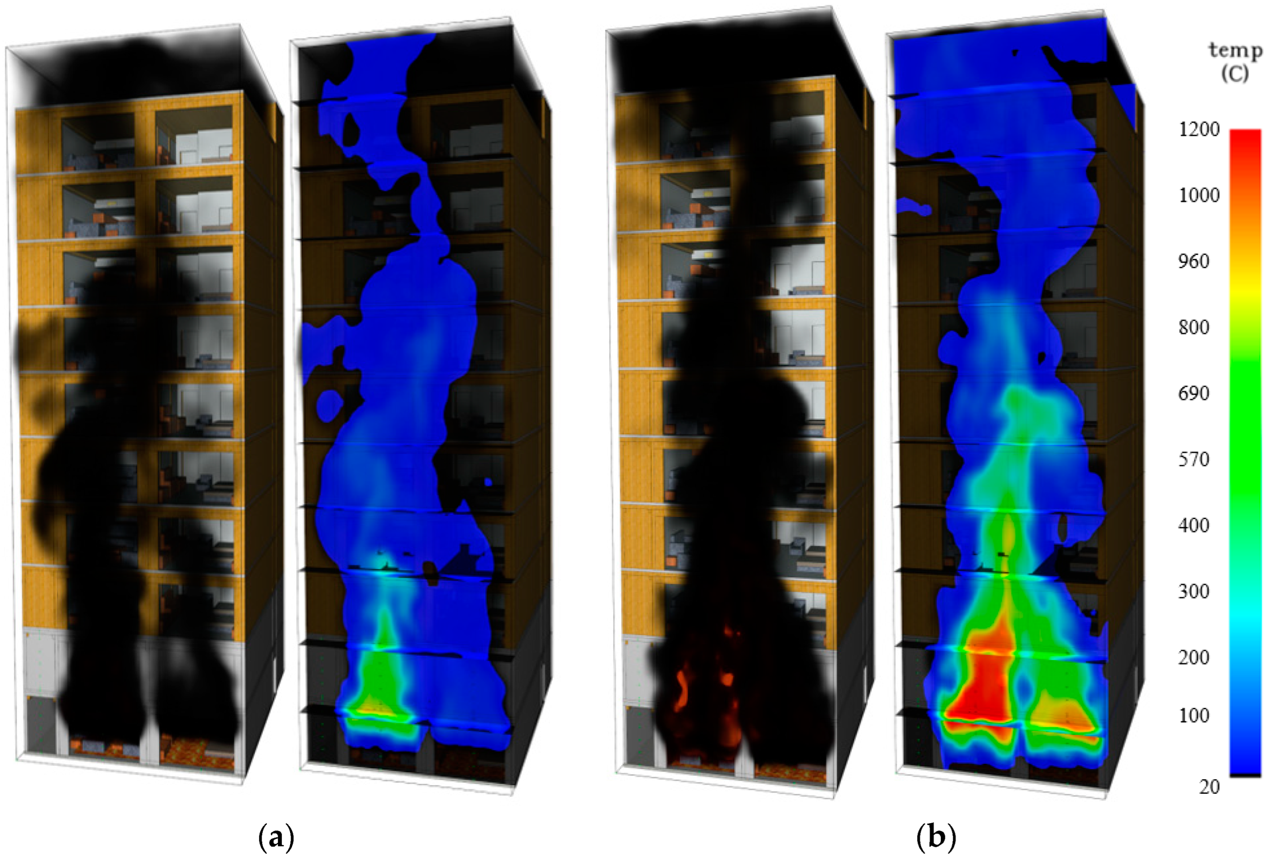
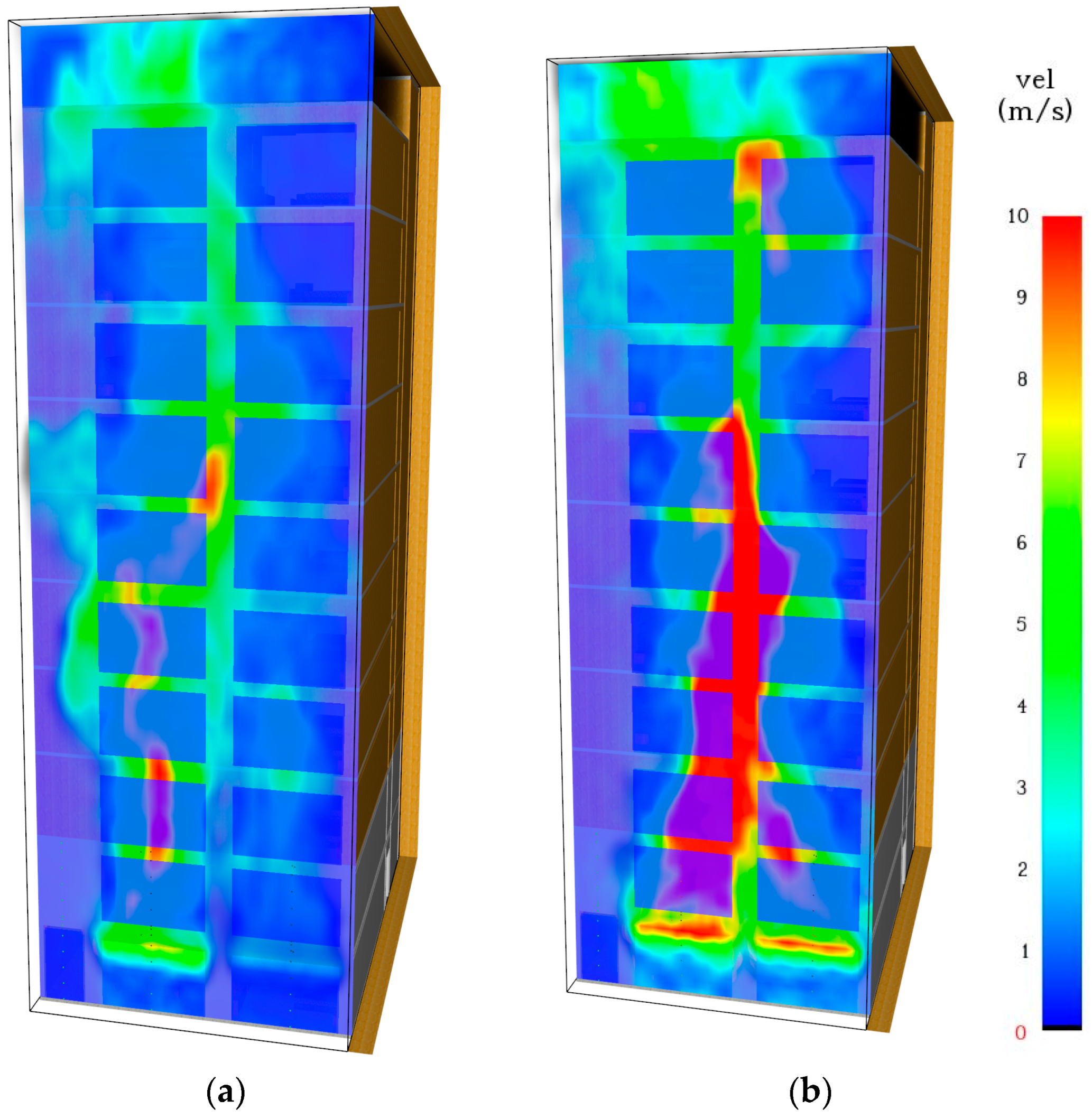
Figure 9 demonstrates temperatures and fire spread outside the building, along wall A (see Figure 1), where Figure 9a,b show predicted models after 14 and 18 min, respectively. Figure 10 shows the velocity contours associated with fire spread outside the CLT building model along wall A: (a) 14 min after the fire ignition (b) 18 min after the fire ignition. It is evident from the velocity contours that the velocity value in the fire is in the range of 5 m/s to 10 m/s; hence, FDS is suitable for the present study.
Comparisons of temperatures as a function of time between the predicted model and experimental data outside the building along wall A at 3 m and 6 m heights are presented in Figure 11 and Figure 12, where locations of thermocouples are shown in red circular points. Figure 11 indicates that the maximum peak temperature recorded for both the prediction and experimental data at height of 3 m was 1100 °C. At the height of 6 m, the peak temperature was 900 °C for both prediction and experimental data. Figure 12 shows comparisons at different heights (3 m and 6 m) above the bedroom, where the temperatures predicted by FDS are almost identical to experimental results.
Temperatures outside the building along wall A, at different heights (9 m, 12 m, 15 m, 18 m) are presented in Figure 13. Red circular points show locations of thermocouples. Predicted results show that temperature decreases from the 3rd to 6th floor by an average of 100–200 °C per floor. However, above 18 m, physically from 6th to 10th floor, only a slight change not exceeding 50 °C in the temperatures was noticed not increase above 50 °C. Figure 13 illustrates that the peak temperature on the 3rd floor at the height of 9 m was 500 °C. The maximum temperature recorded in the thermocouple on the 4th floor (15 m height) was 300 °C. The figure also shows that peak temperature on the 5th and 6th floor was 200 and 100 °C, respectively.
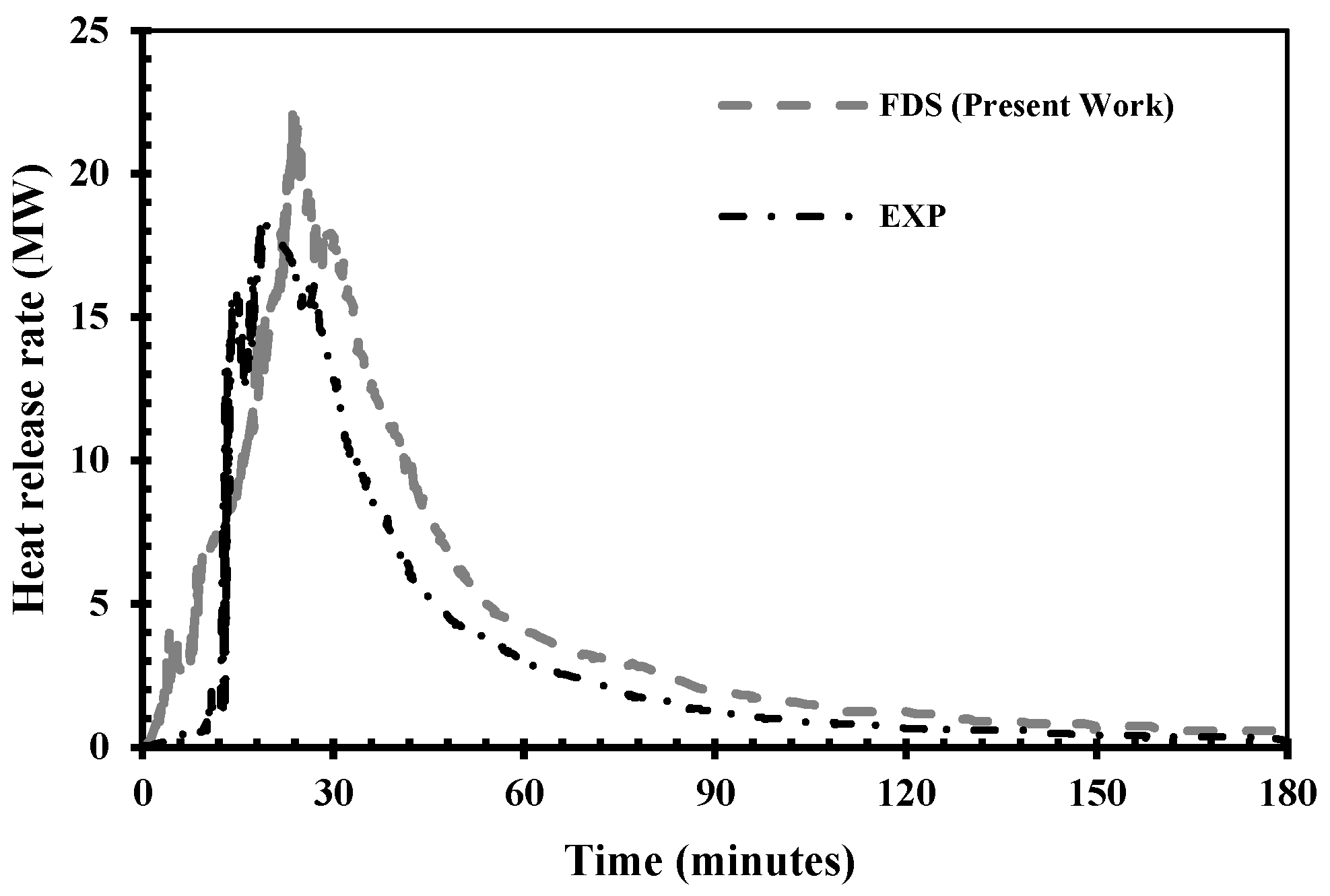
Figure 14 shows the optimal number of grid resolutions for deriving the acceptable curve of HRR of fire as a function of time. The proposed FDS simulation for the HRR is compared with the experimental results. It can be observed from Figure 14 that the curves obtained from the grid resolution of the proposed scheme shows a similar trend of curve with the experimental curve. However, the FDS-based simulation shows some fluctuation. The grid resolution for the proposed simulation was also varied; however, no change was observed on the predicted value of HRR. The predicted maximum value of HRR was 22 MW at approximately 22 min. In experimental results, the HRR peak value was 18.5 MW at 19 min. One reason for this difference may be because the fire products collector (FPC) which was used in the experiment was taken offline to change the gas filter for a certain time during the experiment [23]. Consequently, the FPC hood could not capture all combustion products.
The comparisons of oxygen and carbon dioxide concentrations between experimental data and the present simulation results are shown in Figure 15 and Figure 16. The oxygen gas analyser was placed in the same location in the corridor on all floors, as shown in Figure 1 by the letter N. The experimental result of concentration on the first floor was very close to numerical simulation, as shown in Figure 15. Figure also shows no change in concentration on the second floor. The change in concentration was only on the first floor. No change in concentration was observed between the second to tenth floors, due to the fire activity occurring only on the first floor.
Figure 16 shows that concentration increased at the same time of apartment door failure. The door failure occurred after 62 min in the FDS simulation and 57:54 min in the experiment, as shown in Table 2. The present prediction results and the experimental data showed no change in concentration on the second floor, as shown in Figure 16. This indicates that there was no fire activity on any floor above the first floor. The results show that the present numerical approach can reliably estimate and concentrations in building fire scenarios.
5. Conclusions
Numerical simulations were carried out to study fire scenarios in a multi-storey cross laminated timber (CLT) building. The CFD software FDS v.6.7 was used. Predicted results were validated by comparison with available experimental data. The experimental data were taken from a full-scale test performed on a two-storey CLT residential building. The fire scenarios in the predicted model were the same as in the experiment. Comparison of temperatures in the living room and bedroom showed reasonable agreement with experiments. In the living room, the flashover occurred after 16 min when two thermocouple temperatures reached up to 600 °C. Results showed that the fire spread rapidly in the period between 12–20 min, when the maximum temperature recorded by thermocouples at 1.83 m height was 1100 °C. In the bedroom, flashover occurred after 21 min, with a maximum temperature of 1000 °C recorded. A good agreement was noticed in the living room on the ceiling surface; the maximum temperature recorded on the ceiling surface reached up to 1200 °C, whereas at 12 mm and 70 mm depths were not exceeding 50 °C and 20 °C, respectively. Experimental data of temperatures on wall B, wall D, and ceiling demonstrated good agreement with the predictions. A reasonable agreement between predicted and experimental temperatures outside the building along wall A on the first and second floors at different heights was obtained, where the peak experimental and numerical temperatures above the living room at height 3 m and 6 m were 1100 °C and 900 °C, respectively. On the other side, above the bedroom at the same height, the temperatures were slightly higher than in the living room, at 1300 °C at 3 m and 1000 °C at 6 m height. This variation was attributed to fuel load in the bedroom being higher than in the living room. Present predicted results were almost the same as experimental results. Temperatures along wall A, from the 3rd to 10th floor, were also predicted by numerical simulation. The predicted results showed the temperatures increased rapidly in the period between 12–20 min. At different heights 9 m, 12 m, 15 m and 18 m, the maximum temperature recorded was 500 °C, 300 °C, 200 °C and 100 °C, respectively. The measured temperatures in the remaining floors above the 6th floor, physically at height 21 m, 24 m, 27 m and 30 m, were less than 100 °C. The predicted HRR during the fire compared very well with the experimental data. The concentrations of and were also recorded on all floors in the corridors. The results demonstrated no change in gas concentration on the floors from 2nd to 10th, due to no fire activity occurring on those floors. The comparison of and concentrations in the corridors on the first and second floors showed good agreement. The results indicate that the CFD tools such as Fire Dynamics Simulator can be used for predicting fire scenarios in high-rise CLT buildings.
Author Contributions
Writing—original draft, S.M.H.; Supervision, J.N. All authors have read and agreed to the published version of the manuscript.
Funding
This research received no external funding.
Data Availability Statement
Not applicable.
Conflicts of Interest
The authors declare no conflict of interest.
References
- Buchanan, A.H.; Abu, A.K. Structural Design for Fire Safety; John Wiley & Sons: Hoboken, NJ, USA, 2017. [Google Scholar] [CrossRef]
- Hu, Q.; Dewancker, B.; Zhang, T.; Wongbumru, T. Consumer Attitudes Towards Timber Frame Houses in China. Procedia-Soc. Behav. Sci. 2016, 216, 841–849. [Google Scholar] [CrossRef]
- Brandner, R.; Flatscher, G.; Ringhofer, A.; Schickhofer, G.; Thiel, A. Cross laminated timber (CLT): Overview and development. Eur. J. Wood Wood Prod. 2016, 74, 331–351. [Google Scholar] [CrossRef]
- Abrahamsen, R.B.; Malo, K.A. Structural design and assembly of “Treet”—A 14-storey timber residential building in Norway. In World Conference on Timber Engineering; 2014; Available online: https://wcte2014.ca (accessed on 12 March 2023).
- Walsh, N.P. The Tallest Timber Tower in Australia Opens in Brisbane. 2018. Available online: https://www.archdaily.com/906495/the-tallest-timber-tower-in-australia-opens-in-brisbane (accessed on 12 March 2023).
- Green, J. World’s tallest timber for Australia. Build. Connect. 2012, 20–21. Available online: https://search.informit.org/doi/10.3316/informit.790325717655902 (accessed on 12 March 2023).
- Harrouk, C. The World’s Tallest Hybrid Timber Tower Is under Construction in Sydney, Australia. 2020. Available online: https://www.archdaily.com/942496/the-worlds-tallest-hybrid-timber-tower-is-under-construction-in-sydney-australia (accessed on 12 March 2023).
- Su, J.; Lafrance, P.-S.; Hoehler, M.S.; Bundy, M. Fire Safety Challenges of Tall Wood Buildings–Phase 2: Task 3-Cross Laminated Timber Compartment Fire Tests. 2018. Available online: https://tsapps.nist.gov/publication/get_pdf.cfm?pub_id=925297 (accessed on 12 March 2023).
- Emberley, R.; Putynska, C.G.; Bolanos, A.; Lucherini, A.; Solarte, A.; Soriguer, D.; Gonzalez, M.G.; Humphreys, K.; Hidalgo, J.P.; Maluk, C.; et al. Description of small and large-scale cross laminated timber fire tests. Fire Saf. J. 2017, 91, 327–335. [Google Scholar] [CrossRef]
- Hoehler, M.; Su, J.; Lafrance, P.-S.; Bundy, M. Fire Safety Challenges of Tall Wood Buildings: Large-scale Cross-laminated Timber Compartment Fire Tests. In Proceedings of the SiF 2018-The 10th International Conference on Structures in Fire, Belfast, UK, 6–8 June 2018; New University of Ulster: Belfast, Ireland, 2018. [Google Scholar]
- Gorska, C.; Hidalgo, J.P.; Torero, J.L. Fire dynamics in mass timber compartments. Fire Saf. J. 2020, 120, 103098. [Google Scholar] [CrossRef]
- Fernandes, C.; Fraga, G.; França, F.; Centeno, F. Radiative transfer calculations in fire simulations: An assessment of different gray gas models using the software FDS. Fire Saf. J. 2020, 120, 103103. [Google Scholar] [CrossRef]
- Betting, B.; Varea, E.; Gobin, C.; Godard, G.; Lecordier, B.; Patte-Rouland, B. Experimental and numerical studies of smoke dynamics in a compartment fire. Fire Saf. J. 2019, 108, 102855. [Google Scholar] [CrossRef]
- Hou, L.-F.; Li, M.; Cui, W.-Y.; Liu, Y.-C. Numerical Simulation and Analysis of On-building High-rise Building Fires. Procedia Eng. 2011, 11, 127–134. [Google Scholar] [CrossRef]
- Yi, X.; Lei, C.; Deng, J.; Ma, L.; Fan, J.; Liu, Y.; Bai, L.; Shu, C.-M. Numerical Simulation of Fire Smoke Spread in a Super High-Rise Building for Different Fire Scenarios. Adv. Civ. Eng. 2019, 2019, 1659325. [Google Scholar] [CrossRef]
- Ling, D.; Kan, K. Numerical Simulations on Fire and Analysis of the Spread Characteristics of Smoke in Supermarket. In International Conference on Computer Education, Simulation and Modeling; Springer: Berlin/Heidelberg, Germany, 2011; pp. 7–13. [Google Scholar]
- Rahmani, A.; Salem, M. Simulation of Fire in Super High-Rise Hospitals Using Fire Dynamics Simulator (FDS). Electron. J. Gen. Med. 2020, 17, em200. [Google Scholar] [CrossRef] [PubMed]
- Chen, C.-J.; Hsieh, W.-D.; Hu, W.-C.; Lai, C.-M.; Lin, T.-H. Experimental investigation and numerical simulation of a furnished office fire. Build. Environ. 2010, 45, 2735–2742. [Google Scholar] [CrossRef]
- Wang, M.; Han, X.; Wu, G.; Liu, Q.Q. Simulation Analysis of Temperature Characteristics for a Theater Fire. In Proceedings of the Int Symp on Innovations and Sustainability of Structures in Civil Engineering. 2008, p. 2. Available online: https://iopscience.iop.org/article/10.1088/1742-6596/410/1/011001 (accessed on 12 March 2023).
- McGrattan, K.; Hostikka, S.; McDermott, R.; Floyd, J.; Weinschenk, C.; Overholt, K. Fire Dynamics Simulator User’s Guide; National Institute of Standards and Technology, Building and Fire Research Laboratory: Gaithersburg, MD, USA, 2013; Volume 1019, p. 347. [CrossRef]
- McGrattan, K.B.; McDermott, R.; Weinschenk, C.; Overholt, K.; Hostikka, S.; Floyd, J. Fire Dynamics Simulator Technical Reference Guide, Volume 1 Mathematical Model; Hughes Associates, Inc.: Baltimore, MD, USA, 2013; p. 149. [Google Scholar] [CrossRef]
- Jevtić, R.B. The importance of fire simulation in fire prediction. Tehnika 2014, 69, 153–158. [Google Scholar] [CrossRef]
- Zelinka, S.L.; Hasburgh, L.E.; Bourne, K.J.; Tucholski, D.R.; Ouellette, J.P. Compartment Fire Testing of a Two-Story Mass Timber Building; United States Department of Agriculture, Forest Service, Forest Products Laboratory: Washington, DC, USA, 2018; Volume 247, pp. 1–475. [CrossRef]
- Morgan, J.H.; Gottuk, D.T.; Hall, J.R., Jr.; Harada, K.; Kuligowski, E.D.; Puchovsky, M.; Torero, J.; Watts, J.M., Jr.; Wieczorek, C.J. (Eds.) SFPE Handbook of Fire Protection Engineering; Springer: Berlin/Heidelberg, Germany, 2016. [Google Scholar] [CrossRef]
- Hadden, R.M.; Bartlett, A.I.; Hidalgo, J.P.; Santamaria, S.; Wiesner, F.; Bisby, L.A.; Deeny, S.; Lane, B. Effects of exposed cross laminated timber on compartment fire dynamics. Fire Saf. J. 2017, 91, 480–489. [Google Scholar] [CrossRef]
- Hadjisophocleous, G.; Jia, Q. Comparison of FDS Prediction of Smoke Movement in a 10-Storey Building with Experimental Data. Fire Technol. 2009, 45, 163–177. [Google Scholar] [CrossRef]
- Xiao, B. Comparison of Numerical and Experimental Results of Fire Induced Doorway Flows. Fire Technol. 2012, 48, 595–614. [Google Scholar] [CrossRef]
- Khan, A.A.; Usmani, A.; Torero, J.L. Evolution of fire models for estimating structural fire-resistance. Fire Saf. J. 2021, 124, 103367. [Google Scholar] [CrossRef]
- Cai, N.; Chow, W.-k. Numerical studies on heat release rate in a room fire burning wood and liquid fuel. In Building Simulation; Springer: Berlin/Heidelberg, Germany, 2014; pp. 511–524. [Google Scholar]
- Sharma, T.; He, Y.; Mahendran, M. Lifts for emergency evacuation in apartment buildings. In Fire Safety Science-Proceedings of the Ninth International Symposium; International Association for Fire Safety Science: London, UK, 2008; pp. 1–6. [Google Scholar]
- Cortés, D.; Gil, D.; Azorín, J.; Vandecasteele, F.; Verstockt, S. A Review of Modelling and Simulation Methods for Flashover Prediction in Confined Space Fires. Appl. Sci. 2020, 10, 5609. [Google Scholar] [CrossRef]
- Babrauskas, V. Estimating room flashover potential. Fire Technol. 1980, 16, 94–103. [Google Scholar] [CrossRef]
- Drysdale, D. An Introduction to Fire Dynamics; John Wiley & Sons: New York, NY, USA, 2011. [Google Scholar] [CrossRef]
Figure 1.
Building typical floor plan (present work) with letter (A, B, C, D, E, F, G, H, I, J, K, N) designations for the walls and measurement instruments.
Figure 1.
Building typical floor plan (present work) with letter (A, B, C, D, E, F, G, H, I, J, K, N) designations for the walls and measurement instruments.

Figure 2.
(a) Thermocouples represented as yellow circle points in the first two-storey in two configurations multiple thermocouples placed in a vertical layer at 60 cm apart and single thermocouples placed in each room at various heights and locations. (b) Location of fire source when fire started.

Figure 3.
CLT Building model (present work) (a) divided into computational mesh interconnected blocks and (b) front view with dimensions, where the first two-floor covered by gypsum wallboard as in the experiment [23].
Figure 3.
CLT Building model (present work) (a) divided into computational mesh interconnected blocks and (b) front view with dimensions, where the first two-floor covered by gypsum wallboard as in the experiment [23].

Figure 4.
Comparisons of air temperatures between predicted model (present work) and experimental data [23] at location G (see Figure 1) in living room at 1.83 m height.

Figure 5.
Comparisons of air temperatures between predicted model (present work) and experimental data [23] at location H (see Figure 1) in bedroom at 1.83 m height.

Figure 6.
Comparisons of air temperatures between predicted model (present work) and experimental data [23] on wall B at location J (see Figure 1) in different depths, one at the wall surface and two embedded at depths 12 mm and 70 mm.

Figure 7.
Comparisons of air temperatures between predicted model (present work) and experimental data [23] on wall D at location K (see Figure 1) in different depths, one at the wall surface and two embedded at depths 12 mm and 70 mm.

Figure 8.
Comparisons of temperatures between predicted model (present work) and experimental data [23] at location I (see Figure 1), in living room ceiling, at different depths, one at the wall surface and two embedded.

Figure 9.
Temperatures and fire spread outside CLT building model (present work) along wall A: (a) 14 min after the fire ignition, (b) 18 min after the fire ignition.
Figure 9.
Temperatures and fire spread outside CLT building model (present work) along wall A: (a) 14 min after the fire ignition, (b) 18 min after the fire ignition.

Figure 10.
Velocity contours associated with fire spread outside CLT building model (present work) along wall A: (a) 14 min after the fire ignition (b) 18 min after the fire ignition.
Figure 10.
Velocity contours associated with fire spread outside CLT building model (present work) along wall A: (a) 14 min after the fire ignition (b) 18 min after the fire ignition.

Figure 11.
Comparison of temperatures between predicted model (present work) and experimental data [23] outside the building along wall A (see Figure 1) at different heights (3 m, 6 m) above living room where location of thermocouples in red circular points.

Figure 12.
Comparison of temperatures between predicted model (present work) and experimental data [23] outside the building along wall A (see Figure 1) at different heights (3 m, 6 m) above the bedroom, where the locations of thermocouples in red circular points.

Figure 13.
Temperatures outside the building (present work) along wall A at different heights (9 m, 12 m, 15 m, 18 m).
Figure 13.
Temperatures outside the building (present work) along wall A at different heights (9 m, 12 m, 15 m, 18 m).

Figure 14.
Comparison of heat release rate of the fire between predicted model (present work) and experimental data [23].
Figure 14.
Comparison of heat release rate of the fire between predicted model (present work) and experimental data [23].

Figure 15.
Comparison of oxygen concentration in the corridor in the first two-floor between predicted model (present work) and experimental data [23].
Figure 15.
Comparison of oxygen concentration in the corridor in the first two-floor between predicted model (present work) and experimental data [23].

Figure 16.
Comparison of carbon dioxide concentration in the corridor in first two floor between predicted model (present work) and experimental data [23].
Figure 16.
Comparison of carbon dioxide concentration in the corridor in first two floor between predicted model (present work) and experimental data [23].


Table 1.
Thermal properties of gasoline [24].
Table 1.
Thermal properties of gasoline [24].
| Fuel | Heat of Combustion kJ/g/K | Heat of Reaction KJ/Kg | Boiling Temperature | Soot Yield Factor | CO Yield Factor | |
|---|---|---|---|---|---|---|
| Gasoline | 27.6 | 338.9 | 155 °C | 0.181 | 0.067 | 2.33 |
Table 2.
Flashover incidents versus time.
| Locations | Incidents | (FDS) Present Work (Min) | Experiment [23] (Min) |
|---|---|---|---|
| Living room | Flashover | 16:00 | 13:27 |
| Bedroom | Flashover | 21:00 | 17:20 |
| Corridor | Flame spread outside apartment | 33:00 | 26:51 |
| Apartment door | Failure | 62:00 | 57:54 |
Disclaimer/Publisher’s Note: The statements, opinions and data contained in all publications are solely those of the individual author(s) and contributor(s) and not of MDPI and/or the editor(s). MDPI and/or the editor(s) disclaim responsibility for any injury to people or property resulting from any ideas, methods, instructions or products referred to in the content. |
© 2023 by the authors. Licensee MDPI, Basel, Switzerland. This article is an open access article distributed under the terms and conditions of the Creative Commons Attribution (CC BY) license (https://creativecommons.org/licenses/by/4.0/).
Share and Cite
MDPI and ACS Style
Hayajneh, S.M.; Naser, J. Fire Spread in Multi-Storey Timber Building, a CFD Study. Fluids 2023, 8, 140. https://doi.org/10.3390/fluids8050140
AMA Style
Hayajneh SM, Naser J. Fire Spread in Multi-Storey Timber Building, a CFD Study. Fluids. 2023; 8(5):140. https://doi.org/10.3390/fluids8050140
Chicago/Turabian StyleHayajneh, Suhaib M., and Jamal Naser. 2023. "Fire Spread in Multi-Storey Timber Building, a CFD Study" Fluids 8, no. 5: 140. https://doi.org/10.3390/fluids8050140