

Numerical Study of Flow around Two Circular Cylinders in Tandem, Side-By-Side and Staggered Arrangements

School of Mechanical and Design Engineering, University of Portsmouth, Portsmouth PO1 3DJ, UK
*
Author to whom correspondence should be addressed.
Fluids 2023, 8(5), 148; https://doi.org/10.3390/fluids8050148
Submission received: 31 March 2023
/
Revised: 28 April 2023
/
Accepted: 4 May 2023
/
Published: 7 May 2023
(This article belongs to the Collection Advances in Turbulence)
Abstract
:Simulations are presented for flow around pairs of circular cylinders at a Reynolds number of 3900. The flow is assumed to be two-dimensional and incompressible in nature and the simulations are performed using a RANS (Reynolds Averaged Navier Stokes) approach with a k-ε model. Simulations are performed for three different configurations of the cylinders: A tandem configuration where the line joining the centre of the cylinders is parallel to the mean flow direction; side-by-side, where the centre line is perpendicular to the mean flow direction; and staggered where the centre line is an angle α to the flow direction. Simulation results are presented for cylinder separations ranging from 1.125 to 4 diameters and for values of α between 10° and 60°. The results are presented and discussed in terms of the lift and drag coefficients, the Strouhal number, the vorticity field and the flow regimes observed. The results and flow regimes are also compared to previous observations at lower Reynolds numbers to investigate the Reynolds number dependence of the phenomena.
1. Introduction
The flow around a single circular cylinder has been investigated in detail and it is one of the classical problems of fluid mechanics with the dependence of the flow on the Reynolds number being well established [1,2]. However, when more than one cylinder is placed in the fluid flow, the entire behaviour of the flow becomes more complex, depending not only on the Reynolds number but also on the distance between the cylinders and their orientation to the flow direction. The flow around two circular cylinders has not been studied at the same depth as the flow around a single cylinder. For a two-cylinder configuration, the line joining the centre of the cylinders can be aligned with the flow direction in the following ways: Parallel to the flow direction giving a tandem arrangement; perpendicular to the flow direction giving a side-by-side orientation; or at an intermediate angle, giving a staggered arrangement.
Early studies of tandem configuration were performed by Igarashi [3] in the range of and , where L is the centre-to-centre separation of the cylinders along the flow direction, D is the diameter and Re is the Reynolds number based on the diameter. sensitivity was examined and six flow patterns were identified, which depended on and . These flow patterns were simplified to three regimes by Zhou and Yiu [4]: An “extended-body” regime at where the cylinders act as one bluff body; a “reattachment” regime at where instead of enclosing the downstream cylinder, the shear layers from the upstream cylinder reattach to the downstream cylinder; and a “co-shedding” regime at , where is large enough for Kármán vortex streets to occur behind both cylinders. Sharman et al. [5] performed numerical predictions at for and found , where is the critical spacing between the cylinders, where a sudden significant change in the values of force coefficients and the Strouhal number occurred. Meneghini et al. [6] performed numerical simulation at and found .
In the side-by-side configuration, the effect is less noticeable than in the tandem configuration, and three main flow patterns were identified [7]. In a “single-bluff-body” at , where T is the centre-to-centre separation of the cylinders perpendicular to the flow direction, the cylinders act as a single bluff body. In “biased flow” at , one cylinder has a narrow wake and higher values of shedding frequency, , and drag coefficient, , while the other cylinder has a wider wake and lower values of the same parameters. In “parallel vortex streets” at , the flow field becomes symmetrical, and behind both cylinders, Kármán vortex streets occur with the same . Ng and Ko [8] examined side-by-side cylinders numerically in the range of for and . Out-of-phase and in-phase vortex shedding and a maximum greater than in the single cylinder case were recorded. Sarvghad-Moghaddam et al. [9] used the finite volume approach at and for . For , values of , the time-averaged drag coefficient, and the Strouhal number, , for were found to be and and for were and , respectively. Side-by-side configurations have also been considered recently at higher experimentally by Alam et al. [10] ( and by Wu et al. [11] (using an LES simulation, with the focus of both studies being the flopping behaviour observed. Afgan et al. [12] also performed LES simulations on side-by-side cylinders, at . Afgan et al. also observed flopping behaviour in the flow and at this Reynolds number and identified a “single-bluff-body” at , “biased flow” at , and “parallel vortex streets” at . A 3D DNS simulation was presented by Chen et al. [13] at . Due to the 3D nature of this simulation, the effect of both the 3D structure of the vortices and the finite length of the cylinder could be assessed. Chen et al. determined that due to the transfer of energy from the initial 2D vortices into the third dimension, the vortices were not as strong as in the 2D case and the lift and drag coefficients and shedding frequencies were smaller, indicating that these could be overestimated in a 2D simulation. Additionally, Chen et al. [13] showed that for a cylinder greater than 6D in length, the end effects on the cylinder have minimal influence.
In the staggered configuration, Sumner et al. [14] used flow visualization and PIV in the range of , and , where is the angle between the centre-to-centre line and the flow direction with = 0 corresponding to a tandem orientation and P is the centre-to-centre separation. Nine flow patterns were identified and further grouped into three categories named “single bluff-body flow patterns”, “small-incidence-angle flow patterns” and “large-incidence-angle flow patterns”. Zhou et al. [15] classified four types of behaviour in the range of and . Type 1 occurred for and the cylinders act as a single body with independent of . In type 2, , a single value of was also observed, but the value was dependent on with a sudden change occurring at a critical point in the range of , with the critical , which was dependent on . Type 3 with and had different values of for each cylinder, with the higher value of more sensitive to change in than the other. In type 4, with , the two cylinders have a different at low , where one is below the value for a single cylinder and the other is above. As Re increases, for both cylinders gradually change towards the value of a single cylinder. Wong et al. [16] examined the reliance of flow classification on in the range of for and and found that the transition between different flow regimes have a significant dependency on . Akbari and Price [17] presented simulations of the staggered configuration at , established five flow patterns and obtained consistent results compared with existing experimental data.
Although numerical methods have gradually increased over the past two decades, the flow around two cylinders has not been fully explored due to its complexity. The majority of numerical methods in the literature are restricted to , as opposed to a larger range in experimental studies [7,17,18]. Here we present simulation results for tandem, side-by-side and staggered configurations of two cylinders at within the subcritical regime where data exist for a single cylinder for validation purposes, but where there are limited data for two-cylinder configurations. Additionally, simulations are also presented at lower Reynold numbers to enable a comparison of two-cylinder configurations. The main aim of this work is to provide details of the flow regimes for different arrangements of two circular cylinders and to investigate the Reynolds number dependence of these regimes. This has applications in a wide range of air and water flows involving chimneys, skyscrapers, heat exchangers, bridges, piers, risers between offshore platforms and the ocean bed and electrical transmission lines.
Details of the numerical method applied in this study, including details of the computational grid, are set out in Section 2. In Section 3, the results are presented and discussed. Initially, simulation around a single cylinder is considered a validation case. The three orientations of tandem, side-by-side and staggered are then presented and discussed in Section 3.2.1, Section 3.2.2 and Section 3.2.3, respectively. Finally, Section 4 contains the conclusions drawn from the study. Additionally, a full set of the results for each configuration is presented in the Supplemental Material.
2. Numerical Method
Two-dimensional incompressible simulations were performed using CFD software STAR-CCM+, version 12.06.011. In the laminar regime, the fluid is described by the incompressible Continuity and Navier–Stokes equations:
while in the turbulent regime, we applied the Reynolds Averaged Navier–Stokes (RANS) equations
where and are the fluid velocity and pressure, is the kinematic viscosity, an overbar represents the time-averaged quantity, a prime represents the fluctuating component and summation is assumed over repeated indices. The Reynolds stresses, was modelled by the standard k-ε turbulent model, where
is the Kronecker delta, is the kinetic energy of the fluctuating motion and is the eddy-viscosity. This was modelled as
where the kinetic energy and the dissipation rate, , were modelled as
respectively, and the constants are given by , , and .
When simulating turbulent flow, the RANS approach adopted here is not the only option. Direct Numerical Simulation (DNS) [13] provides a direct solution of the Navier–Stokes equations without the need for a turbulent model, such as the k-ε turbulent model applied here. This is achieved by using a mesh, which is fine enough to capture the smallest length scales present in the turbulence. This comes at a computational cost, for example, the 3D simulations around a single cylinder at presented in [13] took more than a month running on 576 cores with a speed of 2.0 GHz. Large Eddy Simulation (LES) [12] is an alternative approach, which requires an intermediate level of mesh density between that of RANS and DNS, enabling it to directly simulate more of the turbulent flow compared to RANS. LES can produce greater detail of the structures within the wave region, but this also comes at an additional computational cost with a single run for a single cylinder at reported to take core hours [19]. For this reason, RANS is the standard approach in most industrial applications. The accuracy of the RANS approach depends on the turbulent model selected and the values used for the related constants. The performance of the turbulent models differs between applications, Reynolds number and even the required output, and the improvement and development of new turbulent models is an active area of research. In terms of flow past a cylinder, a number of authors have compared the different turbulent models [20,21]. Stringer et al. [20] suggest that the k-ε turbulent model can perform well at lower Reynolds numbers but suggest moving to a k-ω or SST k-ω model at higher Reynolds numbers. Rehman et al. [21] observed that, for the Reynold number considered here, the k-ε model accurately predicted the force coefficients but was less effective at visualising the vortex shedding.
In the present study, the rectangular fluid domain was created with dimensions of by where is the diameter of the cylinder, which was 0.01 m.
A velocity inlet was applied at the upstream boundary with the velocity required to achieve the desired Reynold number. A pressure outlet was set at the downstream boundary and the other two boundaries were set as symmetry planes. The cylinder combination (or single cylinder) was placed with its centre 12D from the inlet and 12.5D from the symmetry planes and had no-slip boundary conditions.
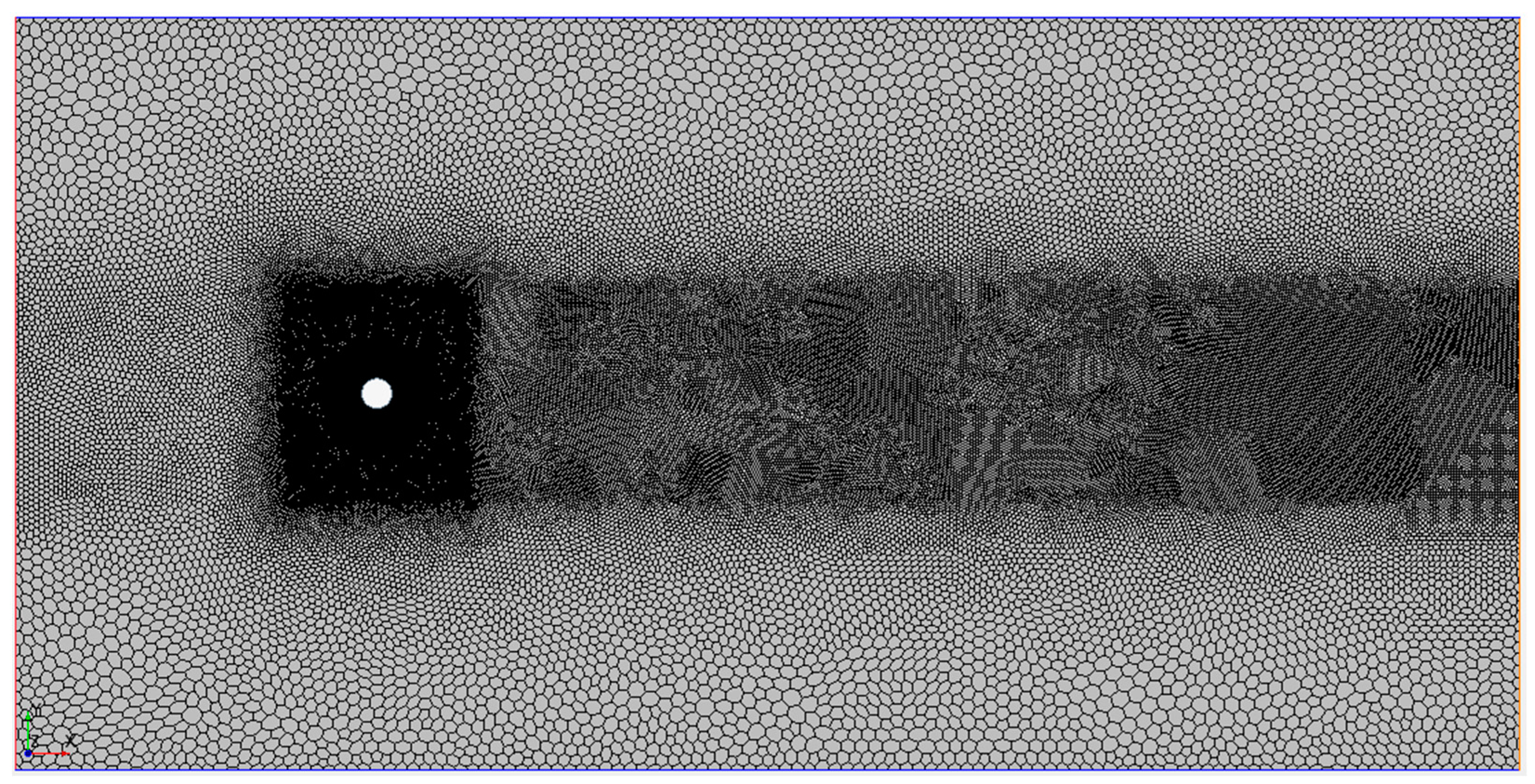
A polygonal mesher was applied to the fluid domain with prism layers around the surface of the cylinder, and the base size of the final mesh was set to 0.0004 m. Four refined regions, VC1, VC2, VC3 and VC4, were set up with relative sizes of and , respectively, compared to the base size, as shown in Figure 1. VC4 is the intersection of two circles of diameter 3D centred on the mid-points of the two cylinders. The dimensions of VC3 were determined such that the nearest point to a cylinder on the horizontal lines was 3.5D and on the vertical lines was 3D. The mesh consists of cells, interior faces and vertices in the case of two cylinders, in the side-by-side configuration, where . For other configurations, the same principle was applied to generate the mesh, but the number of cells, interior faces and vertices changes with the different arrangement of the two cylinders.
For the purpose of validating the accuracy of the results, a mesh convergence study was performed for the flow around a single cylinder at , with respect to and . shown in Table 1 where and represent the percentage differences compared to the finest mesh. Based on these results, a base size of 0.004 m was selected for further simulations. Full details of the mesh are shown in Table 2 and Figure 2.
Following Stringer [20], the prism layer parameters were selected to give Y+ < 1 and to expand to match the cell size in VC4. Figure 3 shows the variation in at where the values are less than one everywhere, with a maximum value of 0.963. This configuration was applied for all considered. The physics models used for the simulations at different of the flow are presented in Table 3.
The liquid used in the simulation was water with the constant density and dynamic viscosity . The temporal discretization of the implicit unsteady solver is set to 2nd-order. The time step was determined based on
where n is the number of cells around the cylinder and U is the speed required to achieve the desired Reynolds number. This gives for . The turbulence specification used in the case of is k-ε, following Rahman et al. [21]. The inlet conditions for the turbulent model were × 10−4 and = × 10−4
3. Results and Discussion
Simulations were performed for the configurations shown in Table 4.
A full set of results in terms of contour maps of the vorticity field, drag and lift coefficient from each cylinder and, where the frequency is not regular, Fourier transforms, are included in the Supplemental Material. Here only the specific results that are pertinent to the discussion are included.
3.1. Single Cylinder
Prior to considering two-cylinder configurations, a range of simulations were run on a single cylinder to validate the numerical approach.
The results of simulations of flow around a single cylinder were as expected, based on the information available in the literature, with decreasing and increasing as increases. Time averaging was applied to the fully developed drag coefficient due to observed fluctuations, the full details of which are presented in the Supplemental Material, where is the time-averaged value .
A comparison of and between the present study and literature data is presented in Table 5 and shows good agreement, indicating the suitability of the model and mesh configurations used in the simulations. For , the in the present study is within the error range of the experimental data [22], and the results from the present study differ from the 2D RANS study by Rahman et al. [21] by 4%. It is approximately 5% smaller than the lowest value found in the 3D LES simulation by Rajani et al. [23] and within the range observed in 3D LES simulations by Ouvrard et al. [24]. The range of values for the LES simulations was due to different models. In terms of its value is larger than the experimental range [22], 2D simulation [21] and 3D LES simulation [23,24] by 4%, 3% 7%, and 0.05%, respectively. This further suggests that the approximations introduced by performing the simulations in 2D and using a RANS approach are acceptable.
3.2. Dual Cylinders
All tandem and side-by-side arrangements were performed at and also at for comparative purposes with numerical reference solutions Meneghini et al. 2001). The staggered arrangements are performed at and are grouped into categories for comparative purposes with the experimental work of Sumner et al. [14] (in the range of ).
3.2.1. Tandem Arrangement
Table 6 shows and for the Downstream Cylinder (DC) and Upstream Cylinder (UC).
In Figure 4, C6 and C7 represent the tandem configuration at . C6 is in the “extended-body” regime, where two cylinders act as one bluff body. The DC is fully submerged in the wake of the UC. In C6, the separated shear layers from the UC are enclosing the DC, without any reattachment onto its surface before the shedding of vortices occurs in the wake of DC, and the gap between cylinders is considered to contain stagnant fluid [7] (Figure 4a). Whereas, in C7, the separated shear layers slightly reattach to the DC, and the fluid in the gap between cylinders is no longer stagnant (Figure 4b). The wake in both cases is narrower and eddies are less compacted than in the single-cylinder cases at the same . The in both cases is positive for the UC and negative for the DC with lower values as increases. The fluctuations increase with Re, but in both cases, the DC fluctuations are higher. Further simulations at lower values of at (see Supplemental Material) were found to remain in the “reattachment” regime, indicating that the “extended body” regime does not exist at this Reynolds number.
C8 and C9 represent the tandem configuration at . C8 is in the “reattachment” regime, where two cylinders are positioned with enough distance between them that the separated shear layers from the UC cannot enclose the DC, but they reattach to the DC [7]. The reattachment of the separated shear layers from the UC to the DC is shown in Figure 5a.
Whereas in C9, vortex shedding is evident from the UC, which indicates the transition to the “co-shedding” regime, where two cylinders are sufficiently far apart for the vortex shedding to occur from UC and DC, as shown in Figure 5b. In C8, the wake of the DC still maintains the pattern observed in C6 at . Whereas in C9, the flow pattern further downstream began to resemble the single-cylinder case. In C8, the of the UC has decreased (compared to C6), but for the DC had increased, while still maintaining a negative value. The negative value of indicates that the DC is still within a low-pressure region created by the separated shear layers from the UC [6]. In C9, the of UC is higher than at , and for the DC has become positive, which is in agreement with approaching the single-cylinder case as the gap increases. The behaviour of the fluctuations is similar to the case of , but in each cylinder, they are higher.
C10 and C11 represent a tandem configuration at . Both cases are now in the transition to the “co-shedding” regime. The UC is shedding vortices in both cases, but the DC is not located entirely outside the UC vortex formation [7], as shown in Figure 6. The eddies in the wake of the DC in C11 are distorted and weaker in terms of magnitude in comparison to C9, which is one of the characteristics of further transition to the “co-shedding” regime [7].
In C10, the of UC had increased to a value close to the single-cylinder case and the of the DC is positive. Whereas in C11, the of the UC maintains the same as at the lower , and of the DC has decreased, in contrast to the same arrangement at .
The results at in C6, C8 and C10 are as expected in comparison to the work performed by Meneghini et al. [6]. The critical value of the gap, where the started to rise, was found to be in the range of , which agrees with the data available in the literature [6]. The results of in C7, C9 and C11 demonstrate the sensitivity of the tandem arrangement to . The was found to be in the range of . The simulation at is in the “reattachment” regime and simulations at and are in the transition to the “co-shedding” regime. Additional simulations at lower (see Supplemental Material) were unable to find a lower limit to the “reattachment” regime indicating that the “extended body” regime does not exist at . This indicates that as Re increases, the range of the gap corresponding to the simplified flow patterns from the work performed by Zhou and Yiu [4] also increases. The in the tandem arrangement are the same for UC and DC in every simulation, and displayed the smallest values of .
3.2.2. Side-by-Side Arrangement
The comparison of and between the present study and literature data in the case of a side-by-side arrangement is presented in Table 7. Agreement with Meneghini et al. [6] is not as close as in the tandem case. The mesh density applied in this study is greater than that used in [6] by approximately an order of magnitude, suggesting that the mesh applied here was appropriate. The side-by-side simulations at were re-run using a refined mesh in VC3 and VC4; however, the results did not change in a significant manner, confirming that the mesh is appropriate. We also note that in the tandem case, only a small discrepancy was observed, suggesting that the discrepancy here is not mesh-dependent. We note that the force data in this arrangement is less regular than in the tandem arrangement, which is discussed below and is evident in the Supplemental Material. It is possible that this may be the cause of the poorer agreements with [6], either due to differences in the averaging approach or a finer mesh being required in [6] to fully capture the phenomenon. We note that the (and ) obtained by Meneghini et al. [6] at and are the same for Higher Cylinder (HC) and Lower Cylinder (LC) in each case, which is in contrast to the present study and Sumner [7]. The results are also compared to Afgan et al. [12], where the data have been extracted from Figures 14 and 15 in [12]. For the Strouhal number, there is reasonable agreement at T = 2D and T = 3D; however, there is a significant discrepancy at T = 1.5D where Afgan et al. [12] reports a significantly different value for the two cylinders. There are differences between the mean drag coefficient reported here at and by Afgan et al. [12] at ; however, they are constant with the decrease in the coefficient with increasing Reynolds number observed in all the results in the table between and .
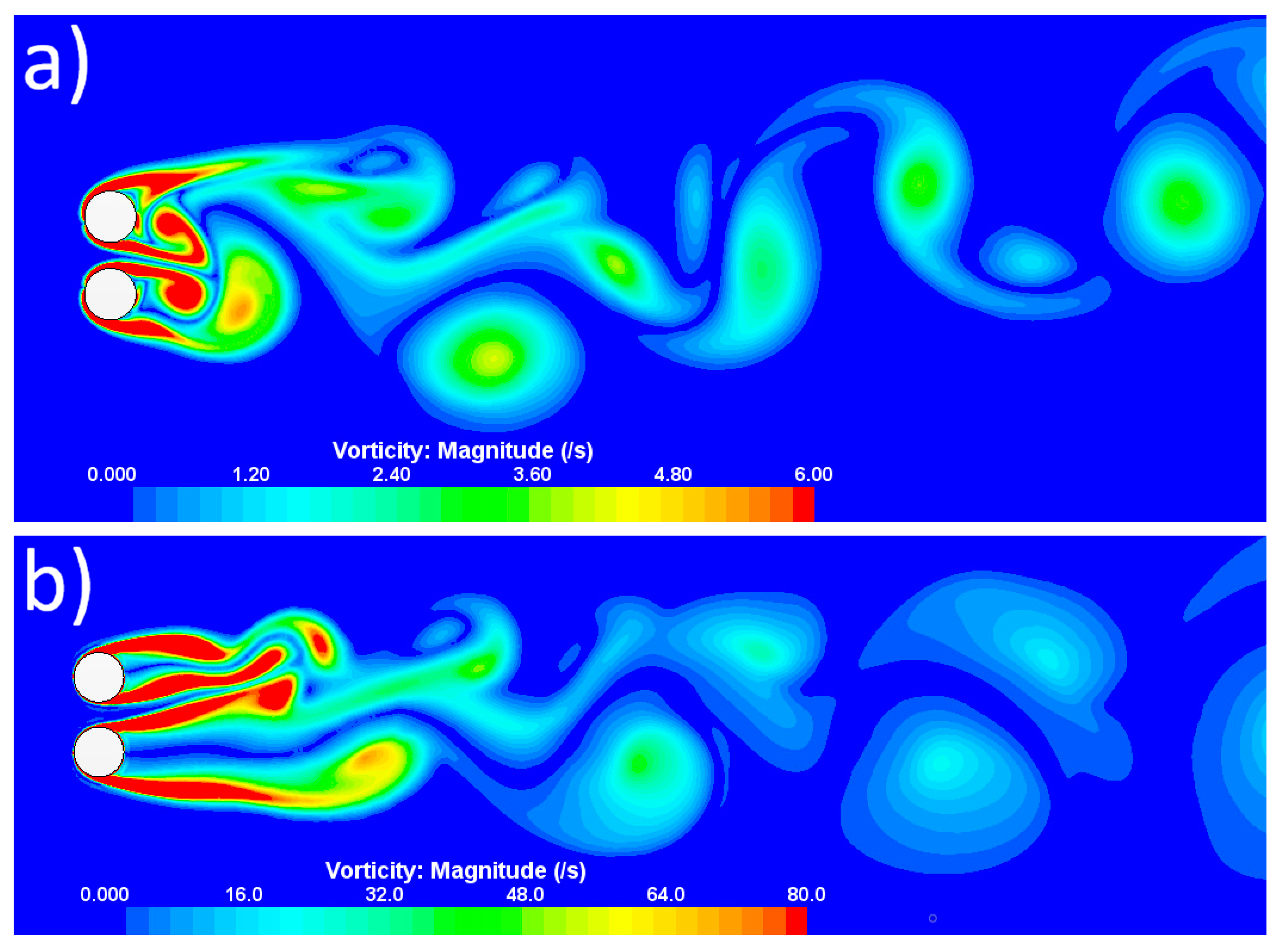
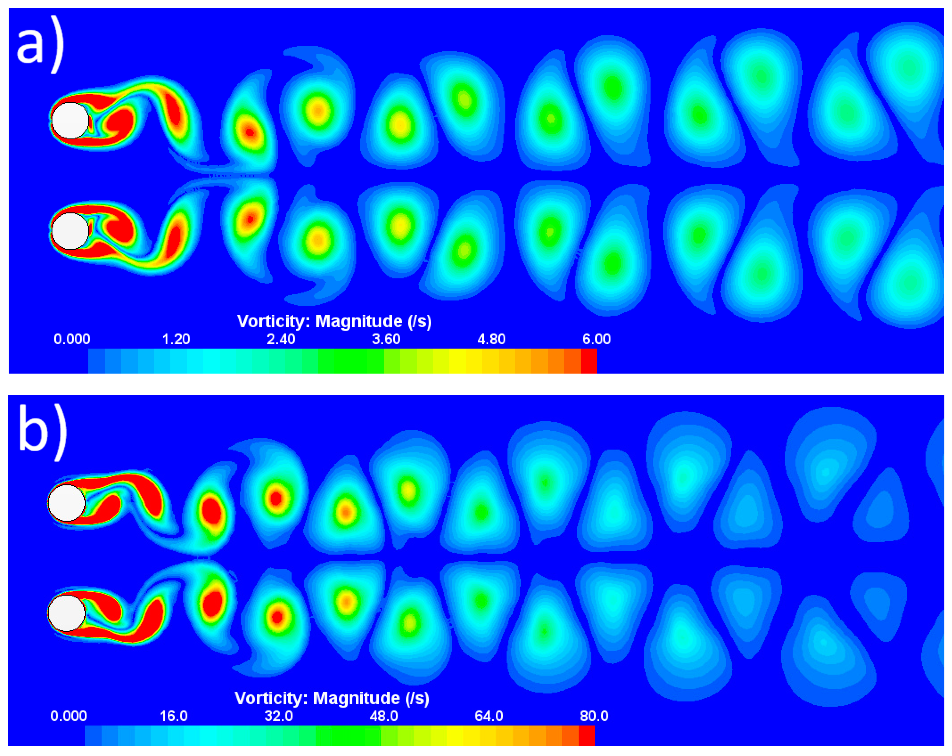
C12 and C13 represent a side-by-side configuration at . Both cases are in the “biased flow” regime, where one cylinder has a narrower wake and higher values of and compared to the other cylinder [7]. In C12, the narrower wake belongs to the LC, but it is not very noticeable from the vorticity contours shown in Figure 7a. Furthermore, the shedding of vortices occurs close to the cylinders, and frontal stagnation points have shifted towards the direction of the gap. In C13, the narrower wake belongs to the HC, which is clearly visible in Figure 7b, and the shedding of vortices is further downstream. In C12, the combined wake is characterized by strong vortices from the outer shear layers, and the deflection of the gap flow changes the direction of the vortices [7]. In C13, the combined wake is not deflected to the same extent, but eddies are distorted.
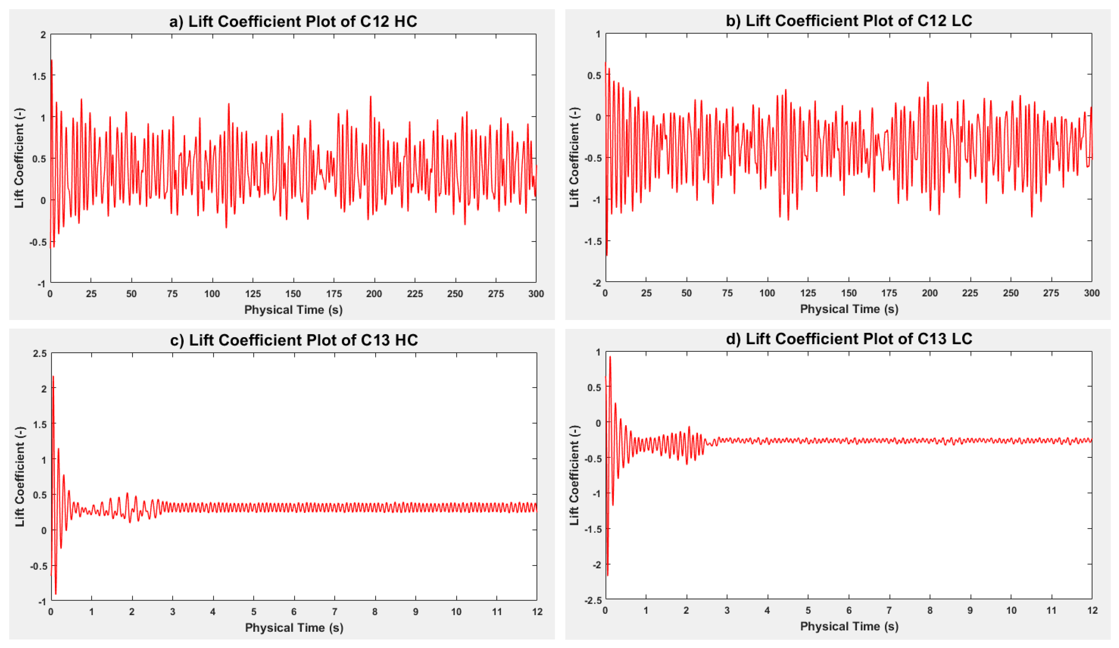
The and plots for both cases are shown in Figure 8 and Figure 9, respectively. They provide evidence of the “flopping” behaviour of the wake, which was described in experimental work performed by Kim and Durbin [29]. The wake is deflected towards one cylinder, which causes its drag to increase [6]. The difference in values between the HC and the LC in C12 is insignificant, as opposed to C13. Whereas in C13, the fluctuations of are lower and more predictable than in C12. In the configuration of , there is a repulsive force acting on both cylinders, which causes to be negative for LC and positive for HC in both cases [6]. The amplitude of is low in C13, which can be explained by inspecting the vorticity contours in Figure 7b. The wake downstream of both cylinders is almost symmetrical before the shedding occurs further downstream.
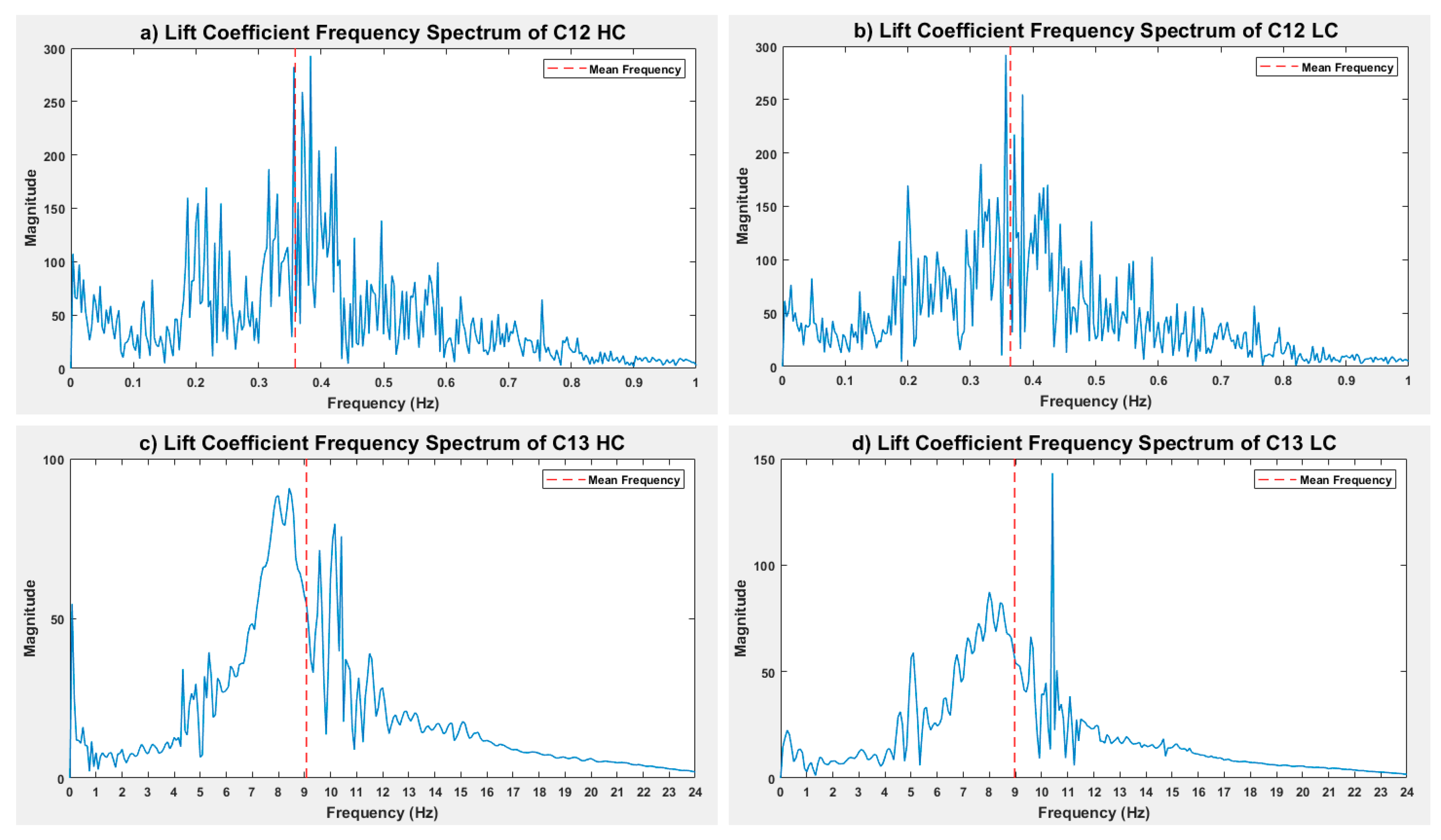
Fourier analysis was performed in Matlab R2018a and is shown in Figure 10. The value for C12 HC, C12 LC, C13 HC and C13 LC was found to be , , and , respectively. The differences between HC and LC are not significant, but the general concept agrees with the work of Sumner [7].
C14 and C15 represent a side-by-side configuration at . Both cases are still in the “biased flow” regime. The vorticity contours for C14 and C15 are shown in Figure 11a and Figure 11b, respectively. In C14, a smaller deflection of the frontal stagnation points towards the gap can be observed. The repulsive force is also smaller, but the wake in both cases is still combined and disorganised [6]. Shedding of vortices in C15 occurs close to the cylinder, unlike in C13.
The “flopping” behaviour of the wake is still present (see Supplemental Material) and shows evidence of a beat-like phenomenon. The values of have increased for every cylinder, which agrees with Meneghini et al. [6].
C16 and C17 represent a side-by-side configuration at . Both cases are in the “parallel vortex streets” regime, and the vorticity contours are shown in Figure 12. The “flopping” was not present for either cylinder in each case, and symmetry was restored, with each cylinder acting more as a single cylinder. However, the interference effects of close proximity still occur. The wakes of both cylinders in each case are synchronized in an anti-phase shedding pattern [7].
The fluctuations are identical for HC and LC in each case, along with . The solutions stabilised but did not regain fluctuations that occur in the single-cylinder case, in agreement with Meneghini et al. [6].
The side-by-side arrangement considered in this study at , in C12, C14 and C16, generally agrees with the work performed by Meneghini et al. [6]. The results at in C13, C15 and C17 show evidence that the side-by-side configuration is not as sensitive to changes in as was found for the tandem configuration and are comparable with the work of Afgan et al. [12], which found the “biased flow” regime at and the “parallel vortex streets” regime at at .
3.2.3. Staggered Arrangement
The values of and for the staggered arrangements are presented in Table 8. C18, C19 and C20 represent staggered configurations for “single bluff-body flow patterns”. C18 is a type 1 single bluff-body (SBB1), C19 is a type 2 single bluff-body (SBB2) and C20 is a base-bleed (BB). C18 is characterised by different lengths of the shear layers. The shear layers from the UC are significantly longer than the ones from the DC. The stretched shear layers are more likely to develop instabilities in the vortex shedding. In C19, the length of the shear layers is similar for both cylinders and the instabilities occur from the UC and the DC, simultaneously. In C20, there is a narrow gap between the cylinders, which allows fluid to flow through the base region. The gap causes stretching of the near-wake region, which causes the vortices to occur further downstream compared to Sumner et al. [14]. The vorticity contours of C18, C19 and C20 are shown in Figure 13a, Figure 13b and Figure 13c, respectively.
C21, C22 and C23 represent staggered configurations of “small-incidence-angle flow patterns”. C21 is a shear layer reattachment (SLR), C22 is an induced separation (IS) and C23 is a vortex impingement (VI). In C21, there is a gap between the cylinders, but the flow through that gap is prevented due to the separated shear layer from the upper side of the UC. This shear layer immediately reattaches onto the DC, which prevents the flow from penetrating the gap. As a result, the flow pattern of the combined wake resembles C18, where the lower shear layer of the UC stretches along the wake downstream, but with weaker magnitude in terms of vorticity and with smaller eddies. In C22, the DC moved further away from the wake of the UC, which allows the upper shear layer of the UC to be directed into the gap between the cylinders. This allows the flow to penetrate the gap and indicates the end of the stretched lower shear layer for the UC from the previous configuration. In C23, the DC is far enough from the UC to allow the shedding of vortices to occur behind both cylinders, which is similar to the “co-shedding” regime in the tandem configuration. The UC started to transition to the behaviour of the single-cylinder case, and the vortices shed from the UC impinge upon the DC [14]. The vorticity contours of C21, C22 and C23 are shown in Figure 14a, Figure 14b and Figure 14c, respectively.
In C23, the fluctuations for have two different peak-to-peak values that repeat every other period, as shown in Figure 15. This is different to the observations for the other cases (see Supplemental Material) and is a sign of instability most likely caused by the vortex shedding from both cylinders with the DC remaining in the wake of the UC. It is worth mentioning that this is not observed for the tandem configuration at at the same , suggesting that this phenomenon is dependent on the angle . No instability was observed in .
C24, C25 and C26 represent the staggered configuration of “large-incidence-angle flow patterns”. C24 is a vortex pairing and enveloping pattern (VPE), C25 is a vortex pairing, splitting and enveloping pattern (VPSE) and C26 is a synchronized vortex shedding pattern (SVS). In C24, the inner shear layers of both cylinders and the vortices created from them further downstream are greatly synchronized, and this phenomenon is called the pairing of gap vortices, which are then enveloped by the vortices formed from the outer shear layer of the UC. In C25, the angle of incidence was doubled, which caused the enveloping to be unfinished due to the increased gap and therefore increased distance between the inner shear layers of both cylinders. The vortices created from those further separated inner shear layers are not well synchronized, as opposed to C24. Gap vortices created from each cylinder split into two different regions of vorticity, which disrupts the enveloping of the outer shear layer of the UC [14]. The vorticity contours of C24 and C25 are shown in Figure 16a and Figure 16b, respectively.
The results for C25 and, to a lesser extent, for C26 (see Supplemental Material) show significantly unstable and unpredictable fluctuations from the UC and the DC, providing evidence of “flopping” behaviour, which was already discussed in the side-by-side arrangement, at and . Fourier analysis of both cylinders in C25 and C26 is shown in Figure 17. The for C25 UC, C25 DC, C26 UC and C26 DC was found to be , , and , respectively. The of the UC in both cases is higher than the DC, which agrees with the discussion in Sumner et al. [14].
For the staggered arrangement considered in this study, the results for the general behaviour of the flow at , in terms of flow patterns, are not dissimilar to the results in Sumner et al. [14], at . The reason for this similarity is most likely due to both studies being in the lower range of the subcritical regime.
C18 is characterized by the highest values of and the lowest values of among all nine flow patterns and where . In C23, at the highest in the present study, the is close to the value for the single cylinder case. C25 and C26 are the only flow patterns in which the “flopping behaviour” can be observed with different values of for each cylinder. The difference between and decreased as the interference effects of close proximity decreased due to an increase in the distance between UC and DC.
4. Conclusions
Two-dimensional simulations of the flow around a single cylinder and two cylinders in various configurations were created using CFD software STAR-CCM+, version 12.06.011. The rectangular fluid domain was created with the dimensions , where . A mesh convergence analysis was conducted for the single cylinder at and the chosen mesh quality was then used for all simulations.
The initial simulations were for flow around a single cylinder at and . The drag coefficient and Strouhal numbers were obtained from these simulations and used to validate the computer model.
Two cylinders were then considered in tandem arrangement, at and for and . The results at were found to be in good agreement with Meneghini et al. [6], providing further validation of the model. The results at showed that tandem arrangement is sensitive to changes. The flow regime at was the “reattachment” regime, and transition to the “co-shedding” regime was observed at and . Additionally, no lower gap limit was found for the “reattachment” indicating that the “extended body” regime does not exist at . In the “reattachment” regime, at , increases as the gap between cylinders decreases.
Two cylinders in the side-by-side arrangement were then presented, at and for and . The results in terms of flow regimes showed that the side-by-side arrangement is not as sensitive to changes as the tandem arrangement. The “biased flow” regime at and , and the “parallel vortex streets” regime at , occurred for both and . Instabilities in the fluctuating forces observed in the “biased flow” provided evidence of flopping behaviour in the wake, which has been observed experimentally [29]. Vortex shedding frequencies were found to be different for the HC and the LC in the “biased flow”. The values of both cylinders at are higher than at , when . However, the for both cylinders at are lower than at when . This shows a level of sensitivity and differences between and the gap ranges for each regime in the side-by-side configuration. In the results at , the interference effects between the cylinders are not as strong as in the “biased flow”. The flopping behaviour was no longer present, and the magnitude of the forces on the cylinders was tending towards the single-cylinder case; however, the wakes of the HC and the LC remained synchronized in an anti-phase shedding pattern. The results in terms of flow patterns were in fairly good agreement with the work performed by Meneghini et al. [6], at . However, in terms of fluctuating forces, differences were observed. In particular, differences were seen in the values of and for and at , in contrast to the result of Meneghini et al. [6] where the same for HC and LC was reported in both cases. At , larger differences between the averaged coefficients of the two cylinders indicate a dependence on as well as the gap.
The final simulations are related to the staggered arrangement at . The flow patterns were grouped into three categories to compare them with the experimental study performed by Sumner et al. [14], in the range of . The results showed that in terms of flow patterns and general behaviour of the flow, they are similar to the results at lower Reynolds numbers. This may be due to both studies being in the lower range of the subcritical regime. The key findings in the staggered configuration were that in the first group of flow patterns, at , the highest value of was found, along with the lowest value of , and this was the only configuration where . In the second group of flow patterns, at , the cylinders are so far apart that the is close to the single cylinder case. In the third group of flow patterns, at and , flopping behaviour was observed along with different values of for each cylinder. The of the UC in both cases is higher than the DC.
Supplementary Materials
The following supporting information can be downloaded at: https://www.mdpi.com/article/10.3390/fluids8050148/s1, A full set of results for each case, in terms of contour maps of the vorticity field, drag and lift coefficient from each cylinder and, where the frequency is not regular, Fourier transforms, are included in the Supplemental Material. Additionally, simulation results for and are also shown indicating that the “extended body” regime does not exist at .
Author Contributions
Conceptualization, J.M.B.; methodology, G.M.S. and J.M.B.; software, G.M.S.; validation, G.M.S.; formal analysis, G.M.S.; investigation, G.M.S.; resources, J.M.B.; data curation, G.M.S.; writing—original draft preparation, G.M.S.; writing—review and editing, G.M.S. and J.M.B.; visualization, G.M.S.; supervision, J.M.B.; project administration, J.M.B. All authors have read and agreed to the published version of the manuscript.
Funding
This research received no external funding.
Data Availability Statement
The data presented in this study are available upon request from the corresponding author.
Conflicts of Interest
The authors declare no conflict of interest.
References
- Derakhshandeh, J.F.; Alam, M.M. A review of bluff body wakes. Ocean Eng. 2019, 182, 475–488. [Google Scholar] [CrossRef]
- Nakayama, Y.; Boucher, R.; Izawa, K. Introduction to Fluid Mechanics; Elsevier Science & Technology: Oxford, UK, 1998. [Google Scholar]
- Igarashi, T. Characteristics of the flow around two circular cylinders arranged in tandem (1st Report). Bull. JSME 1981, 24, 323–331. [Google Scholar] [CrossRef]
- Zhou, Y.; Yiu, M.W. Flow structure, momentum and heat transport in a two-tandem-cylinder wake. J. Fluid Mech. 2006, 548, 17–48. [Google Scholar] [CrossRef]
- Sharman, B.; Lien, F.S.; Davidson, L.; Norberg, C. Numerical predictions of low Reynolds number flows over two tandem circular cylinders. Int. J. Numer. Methods Fluids 2005, 47, 423–447. [Google Scholar] [CrossRef]
- Meneghini, J.R.; Saltara, F.; Siqueira, C.L.R.; Ferrari, J.A., Jr. Numerical Simulation of Flow Interference Between Two Circular Cylinders in Tandem and Side-by-Side Arrangements. J. Fluids Struct. 2001, 15, 327–350. [Google Scholar] [CrossRef]
- Sumner, D. Two circular cylinders in cross-flow: A review. J. Fluids Struct. 2010, 26, 849–899. [Google Scholar] [CrossRef]
- Ng, C.W.; Ko, N.W.M. Flow interaction behind two circular cylinders of equal diameter—A numerical study. J. Wind. Eng. Ind. Aerodyn. 1995, 54–55, 277–287. [Google Scholar] [CrossRef]
- Sarvghad-Moghaddam, H.; Nooredin, N.; Ghadiri-Dehkordi, B. Numerical simulation of flow over two side-by-side circular cylinders. J. Hydrodyn. 2011, 23, 792–805. [Google Scholar] [CrossRef]
- Alam, M.M.; Moriya, M.; Sakamoto, H. Aerodynamic characteristics of two side-by-side circular cylinders and application of wavelet analysis on the switching phenomenon. J. Fluids Struct. 2003, 18, 325–346. [Google Scholar] [CrossRef]
- Wu, G.; Lin, W.; Du, X.; Shi, C.; Zhu, J. On the flip-flopping phenomenon of two side-by-side circular cylinders at a high subcritical Reynolds number of 1.4 × 10⁵. Phys. Fluids 2020, 32, 094112. [Google Scholar] [CrossRef]
- Afgan, I.; Kahil, Y.; Benhamadouche, S.; Sagaut, P. Large eddy simulation of the flow around single and two side-by-side cylinders at subcritical Reynolds numbers. Phys. Fluids 2011, 23, 075101. [Google Scholar] [CrossRef]
- Chen, W.; Ji, C.; Alam, M.M.; Yan, Y. Three-dimensional flow past two stationary side-by-side circular cylinders. Ocean Eng. 2022, 244, 110379. [Google Scholar] [CrossRef]
- Sumner, D.; Price, S.J.; Païdoussis, M.P. Flow-pattern identification for two staggered circular cylinders in cross-flow. J. Fluid Mech. 2000, 411, 263–303. [Google Scholar] [CrossRef]
- Zhou, Y.; Feng, S.X.; Alam, M.M.; Bai, H.L. Reynolds number effect on the wake of two staggered cylinders. Phys. Fluids 2009, 21, 125105. [Google Scholar] [CrossRef]
- Wong, C.W.; Zhou, Y.; Alam, M.M.; Zhou, T.M. Dependence of flow classification on the Reynolds number for a two-cylinder wake. J. Fluids Struct. 2014, 49, 485–497. [Google Scholar] [CrossRef]
- Akbari, M.H.; Price, S.J. Numerical investigation of flow patterns for staggered cylinder pairs in cross-flow. J. Fluids Struct. 2005, 20, 533–554. [Google Scholar] [CrossRef]
- Zhou, Y.; Alam, M.M. Wake of two interacting circular cylinders: A review. Int. J. Heat Fluid Flow 2016, 62, 510–537. [Google Scholar] [CrossRef]
- Jiang, H.; Cheng, L. Large-eddy simulation of flow past a circular cylinder for Reynolds numbers 400 to 3900. Phys. Fluids 2021, 33, 034119. [Google Scholar] [CrossRef]
- Stringer, R.M.; Zang, J.; Hillis, A.J. Unsteady RANS computations of flow around a circular cylinder for a wide range of Reynolds numbers. Ocean. Eng. 2014, 87, 1–9. [Google Scholar] [CrossRef]
- Rahman, M.M.; Karim, M.M.; Alim, M.A. Numerical investigation of unsteady flow past a circular cylinder using 2-D finite volume method. J. Nav. Archit. Mar. Eng. 2007, 4, 27–42. [Google Scholar] [CrossRef]
- Norberg, C. Effects of Reynolds Number and a Low-Intensity Freestream Turbulence on the Flow Around a Circular Cylinder; Chalmers University of Technology: Göteborg, Sweden, 1987; Available online: https://portal.research.lu.se/en/publications/3d112379-5cc5-4935-a097-6f195d9618f7 (accessed on 31 March 2023).
- Rajani, B.N.; Kandasamy, A.; Majumdar, S. LES of Flow past Circular Cylinder at Re = 3900. J. Appl. Fluid Mech. 2016, 9, 1421–1435. [Google Scholar] [CrossRef]
- Ouvrard, H.; Koobus, B.; Dervieux, A.; Salvetti, M.V. Classical and variational multiscale LES of the flow around a circular cylinder on unstructured grids. Comput. Fluids 2010, 39, 1083–1094. [Google Scholar] [CrossRef]
- Tritton, D.J. Experiments on the flow past a circular cylinder at low Reynolds numbers. J. Fluid Mech. 1959, 6, 547–567. [Google Scholar] [CrossRef]
- Ding, H.; Shu, C.; Cai, Q.D. Applications of stencil-adaptive finite difference method to incompressible viscous flows with curved boundary. Comput. Fluids 2007, 36, 786–793. [Google Scholar] [CrossRef]
- Franke, R.; Rodi, W.; Schönung, B. Numerical Calculation of Laminar Vortex-Shedding Flow Past Cylinders. J. Wind Eng. Ind. Aerodyn. 1990, 35, 237–257. [Google Scholar] [CrossRef]
- Braza, M.; Chassaing, P.; Minh, H. Numerical study and physical analysis of the pressure and velocity fields in the near wake of a circular cylinder. J. Fluid Mech. 1986, 165, 79–130. [Google Scholar] [CrossRef]
- Kim, H.; Durbin, P. Investigation of the flow between a pair of circular cylinders in the flopping regime. J. Fluid Mech. 1988, 196, 431–448. [Google Scholar] [CrossRef]
Figure 1.
Volumetric control dimensions and placement within the fluid domain mesh for the flow around two cylinders in the side-by-side configuration, where (not to scale).
Figure 1.
Volumetric control dimensions and placement within the fluid domain mesh for the flow around two cylinders in the side-by-side configuration, where (not to scale).

Figure 2.
The final generated mesh for flow around single cylinder.

Figure 3.
Wall Y+ plot of upper and lower surface of the single cylinder at .

Figure 4.
Vorticity contours of: (a) C6 at ; (b) C7 at .

Figure 5.
Vorticity contours of (a) C8 at ; (b) C9 at .

Figure 6.
Vorticity contours of (a) C10 at ; (b) C11 at .

Figure 7.
Vorticity contours of (a) C12 at ; (b) C13 at .

Figure 8.
Drag coefficient plot of (a) C12 HC at ; (b) C12 LC at ; (c) C13 HC at ; (d) C13 LC at .

Figure 9.
Lift coefficient plot of (a) C12 HC at ; (b) C12 LC at ; (c) C13 HC at ; (d) C13 LC at .

Figure 10.
Lift coefficient frequency spectrum plot of (a) C12 HC at ; (b) C12 LC at ; (c) C13 HC at ; (d) C13 LC at .
Figure 10.
Lift coefficient frequency spectrum plot of (a) C12 HC at ; (b) C12 LC at ; (c) C13 HC at ; (d) C13 LC at .

Figure 11.
Vorticity contours of (a) C14 at ; (b) C15 at .

Figure 12.
Vorticity contours of (a) C16 at ; (b) C17 at .

Figure 13.
Vorticity contours of single bluff-body flow patterns at of (a) C18 at ; (b) C19 at ; (c) C20 at .
Figure 13.
Vorticity contours of single bluff-body flow patterns at of (a) C18 at ; (b) C19 at ; (c) C20 at .

Figure 14.
Vorticity contours of small-incidence-angle flow patterns at of: (a) C21 at ; (b) C22 at ; (c) C23 at .
Figure 14.
Vorticity contours of small-incidence-angle flow patterns at of: (a) C21 at ; (b) C22 at ; (c) C23 at .

Figure 15.
Drag coefficient plot at of: (a) C21; (b) C22; (c) C23 UC; (d) C23 DC.

Figure 16.
Vorticity contours of large-incidence-angle flow patterns at of (a) C24 at ; (b) C25 at ; (c) C26 at .
Figure 16.
Vorticity contours of large-incidence-angle flow patterns at of (a) C24 at ; (b) C25 at ; (c) C26 at .

Figure 17.
Lift coefficient frequency spectrum plot at of: (a) C25 UC; (b) C25 DC; (c) C26 UC; (d) C26 DC.
Figure 17.
Lift coefficient frequency spectrum plot at of: (a) C25 UC; (b) C25 DC; (c) C26 UC; (d) C26 DC.


Table 1.
Mesh convergence data for the flow around a cylinder at .
| Base Size [m] | ||||
|---|---|---|---|---|
| −0.05% | ||||
| −0.03% | ||||
| −0.02% | ||||
| −0.03% | ||||
| 0.00% | ||||
| 0.00% | ||||
| −0.01% | ||||
| - | - |
Table 2.
Details of the mesh controls and volume controls used to generate mesh.
| Control | Value | Control | Value |
|---|---|---|---|
| Base Size | Volumetric Control 1 | ||
| Surface Growth Rate | Volumetric Control 2 | ||
| Number of Prism Layers | Volumetric Control 3 | ||
| Prism Layer Stretching | Volumetric Control 4 | ||
| Prism Layer Total Thickness |
Table 3.
Physics models used for the simulations at different of the flow.
| Model | Reynolds Number | ||
|---|---|---|---|
| 2040 | 80,200 | 3900 | |
| Space | Two-Dimensional | ||
| Time | Steady | Implicit Unsteady | |
| Material | Liquid | ||
| Flow | Segregated Flow | ||
| Equation of State | Constant Density | ||
| Viscous Regime | Laminar | Turbulent | |
| RANS Model | N/A | k-ε | |
| Near Wall Treatment | N/A | Enhanced Wall Treatment | |
Table 4.
Details of simulation configurations.
| Case | Type | L/T/P | α(deg) | Case | Type | L/T/P | α(deg) | ||
|---|---|---|---|---|---|---|---|---|---|
| C1 | 20 | Single | - | - | C14 | 200 | S-by-S | T = 2D | - |
| C2 | 40 | Single | - | - | C15 | 3900 | S-by-S | T= 2D | - |
| C3 | 80 | Single | - | - | C16 | 200 | S-by-S | T = 3D | - |
| C4 | 200 | Single | - | - | C17 | 3900 | S-by-S | T = 3D | - |
| C5 | 3900 | Single | - | - | C18 | 3900 | Staggered | P = 1D | 30 |
| C6 | 200 | Tandem | L = 1.5D | - | C19 | 3900 | Staggered | P = 1D | 60 |
| C7 | 3900 | Tandem | L = 1.5D | - | C20 | 3900 | Staggered | P = 1.125D | 60 |
| C8 | 200 | Tandem | L = 3D | - | C21 | 3900 | Staggered | P = 1.5D | 10 |
| C9 | 3900 | Tandem | L = 3D | - | C22 | 3900 | Staggered | P = 1.5D | 20 |
| C10 | 200 | Tandem | L = 4D | - | C23 | 3900 | Staggered | P = 4D | 10 |
| C11 | 3900 | Tandem | L = 4D | - | C24 | 3900 | Staggered | P = 1.5D | 30 |
| C12 | 200 | S-by-S | T = 1.5D | - | C25 | 3900 | Staggered | P = 1.5D | 60 |
| C13 | 3900 | S-by-S | T = 1.5D | - | C26 | 3900 | Staggered | P = 2.5D | 50 |
Table 5.
Comparison between experimental and numerical results from literature and present study for and in the flow around single cylinder.
Table 5.
Comparison between experimental and numerical results from literature and present study for and in the flow around single cylinder.
| Case | C1 | C2 | C3 | C4 | C5 | |||
|---|---|---|---|---|---|---|---|---|
| 3900 | ||||||||
| Parameters | ||||||||
| Exp. Tritton [25] | - | - | - | - | ||||
| Ding et al. [26] | - | - | - | - | - | - | ||
| Franke et al. [27] | - | - | - | - | ||||
| Braza et al. [28] | - | - | - | - | ||||
| Meneghini et al. [6] | - | - | - | - | - | - | ||
| Exp. Norberg [22] | - | - | - | - | - | - | ||
| 2D Rahman et al. [21] | - | - | - | - | - | - | ||
| 3D LES Rajani et al. [23] | - | - | - | - | - | - | ||
| 3D LES Ouvrard et al. [24] | - | - | - | - | - | - | ||
| Present Study | ||||||||
Table 6.
Comparison between numerical literature results at and present study at and for and for two cylinders in the tandem arrangement.
Table 6.
Comparison between numerical literature results at and present study at and for and for two cylinders in the tandem arrangement.
| Gap L | 1.5 D | 3.0 D | 4.0 D | |||||||||
|---|---|---|---|---|---|---|---|---|---|---|---|---|
| Parameters | ||||||||||||
| Meneghini et al. [6] | ||||||||||||
Table 7.
Comparison between numerical literature results at and and the present study at and for and for two cylinders, in side-by-side arrangement.
Table 7.
Comparison between numerical literature results at and and the present study at and for and for two cylinders, in side-by-side arrangement.
| Gap T | 1.5 D | 2.0 D | 3.0 D | |||||||||
|---|---|---|---|---|---|---|---|---|---|---|---|---|
| Parameters | ||||||||||||
| Meneghini et al. [6] | 1.32 | 1.32 | - | - | 1.42 | 1.42 | - | - | 1.34 | 1.34 | ||
| 1.55 | 1.57 | 0.201 | 0.204 | 1.58 | 1.63 | 0.216 | 0.223 | 1.56 | 1.56 | 0.214 | 0.214 | |
| 1.13 | 0.96 | 0.261 | 0.258 | 1.22 | 1.15 | 0.244 | 0.241 | 1.10 | 1.10 | 0.238 | 0.238 | |
| Afgan et al. [12] | 1.4 | 1.2 | 0.39 | 0.11 | 1.3 | 1.3 | 0.24 | 0.22 | 1.4 | 1.4 | 0.23 | 0.23 |
Table 8.
Numerical results of and for single bluff-body flow patterns from present study at in the flow around two cylinders, in staggered arrangement.
Table 8.
Numerical results of and for single bluff-body flow patterns from present study at in the flow around two cylinders, in staggered arrangement.
| P, α, Case | C18 | C19 | C20 | |||||||||
| Parameter | ||||||||||||
| Value | ||||||||||||
| P, α, case | , C21 | C22 | , C23 | |||||||||
| Parameter | ||||||||||||
| Value | ||||||||||||
| P, α, case | , C24 | C25 | , C26 | |||||||||
| Parameter | ||||||||||||
| Value | ||||||||||||
Disclaimer/Publisher’s Note: The statements, opinions and data contained in all publications are solely those of the individual author(s) and contributor(s) and not of MDPI and/or the editor(s). MDPI and/or the editor(s) disclaim responsibility for any injury to people or property resulting from any ideas, methods, instructions or products referred to in the content. |
© 2023 by the authors. Licensee MDPI, Basel, Switzerland. This article is an open access article distributed under the terms and conditions of the Creative Commons Attribution (CC BY) license (https://creativecommons.org/licenses/by/4.0/).
Share and Cite
MDPI and ACS Style
Skonecki, G.M.; Buick, J.M. Numerical Study of Flow around Two Circular Cylinders in Tandem, Side-By-Side and Staggered Arrangements. Fluids 2023, 8, 148. https://doi.org/10.3390/fluids8050148
AMA Style
Skonecki GM, Buick JM. Numerical Study of Flow around Two Circular Cylinders in Tandem, Side-By-Side and Staggered Arrangements. Fluids. 2023; 8(5):148. https://doi.org/10.3390/fluids8050148
Chicago/Turabian StyleSkonecki, Gracjan M., and James M. Buick. 2023. "Numerical Study of Flow around Two Circular Cylinders in Tandem, Side-By-Side and Staggered Arrangements" Fluids 8, no. 5: 148. https://doi.org/10.3390/fluids8050148