
Rapid Hydrate Formation Conditions Prediction in Acid Gas Streams
by
 , ,
, ,
Anna Samnioti
1,
Eirini Maria Kanakaki
1,
Sofianos Panagiotis Fotias
1 and
Vassilis Gaganis
1,2,* 1
School of Mining and Metallurgical Engineering, National Technical University of Athens, 15780 Athens, Greece
2
Institute of Geoenergy, Foundation for Research and Technology-Hellas, 73100 Chania, Greece
*
Author to whom correspondence should be addressed.
Fluids 2023, 8(8), 226; https://doi.org/10.3390/fluids8080226
Submission received: 2 July 2023
/
Revised: 28 July 2023
/
Accepted: 3 August 2023
/
Published: 5 August 2023
(This article belongs to the Special Issue Multiphase Flow and Granular Mechanics)
Abstract
:Sour gas in hydrocarbon reservoirs contains significant amounts of H2S and smaller amounts of CO2. To minimize operational costs, meet air emission standards and increase oil recovery, operators revert to acid gas (re-)injection into the reservoir rather than treating H2S in Claus units. This process requires the pressurization of the acid gas, which, when combined with low-temperature conditions prevailing in subsurface pipelines, often leads to the formation of hydrates that can potentially block the fluid flow. Therefore, hydrates formation must be checked at each pipeline segment and for each timestep during a flow simulation, for any varying composition, pressure and temperature, leading to millions of calculations that become more intense when transience is considered. Such calculations are time-consuming as they incorporate the van der Walls–Platteeuw and Langmuir adsorption theory, combined with complex EoS models to account for the polarity of the fluid phases (water, inhibitors). The formation pressure is obtained by solving an iterative multiphase equilibrium problem, which takes a considerable amount of CPU time only to provide a binary answer (hydrates/no hydrates). To accelerate such calculations, a set of classifiers is developed to answer whether the prevailing conditions lie to the left (hydrates) or the right-hand (no hydrates) side of the P-T phase envelope. Results are provided in a fast, direct, non-iterative way, for any possible conditions. A set of hydrate formation “yes/no” points, generated offline using conventional approaches, are utilized for the classifier’s training. The model is applicable to any acid gas flow problem and for any prevailing conditions to eliminate the CPU time of multiphase equilibrium calculations.
1. Introduction
Many hydrocarbon reservoirs contain a considerable amount of H2S and, potentially, CO2 content, which has to be separated at gas plants by isolating the acid content from the hydrocarbons in amine units. This way, a natural “sweet” gas product is formed with specifications appropriate for transport to a variety of end users or for on-site consumption for operation energy demands [1,2]. Acid gas is composed mainly of H2S and/or CO2, water vapor, arriving from the sour gas sweetening process, and contaminants such as small amounts of methane and heavier hydrocarbons [3]. Typically, the resulting acid gas waste stream is processed in sulfur recovery units (SRUs), such as the Claus unit, where H2S is converted to elemental sulfur [2,4]. However, SRUs are not a major revenue generator due to the economically unattractive sulfur market price, whereas, air emission standards and regulatory authorities are becoming increasingly strict. As a result, oil and gas operators face an expanding economic burden and are in search of environment-friendly and cost-effective alternative methods for dealing with acid gases produced in association with sour natural resources [1,5].
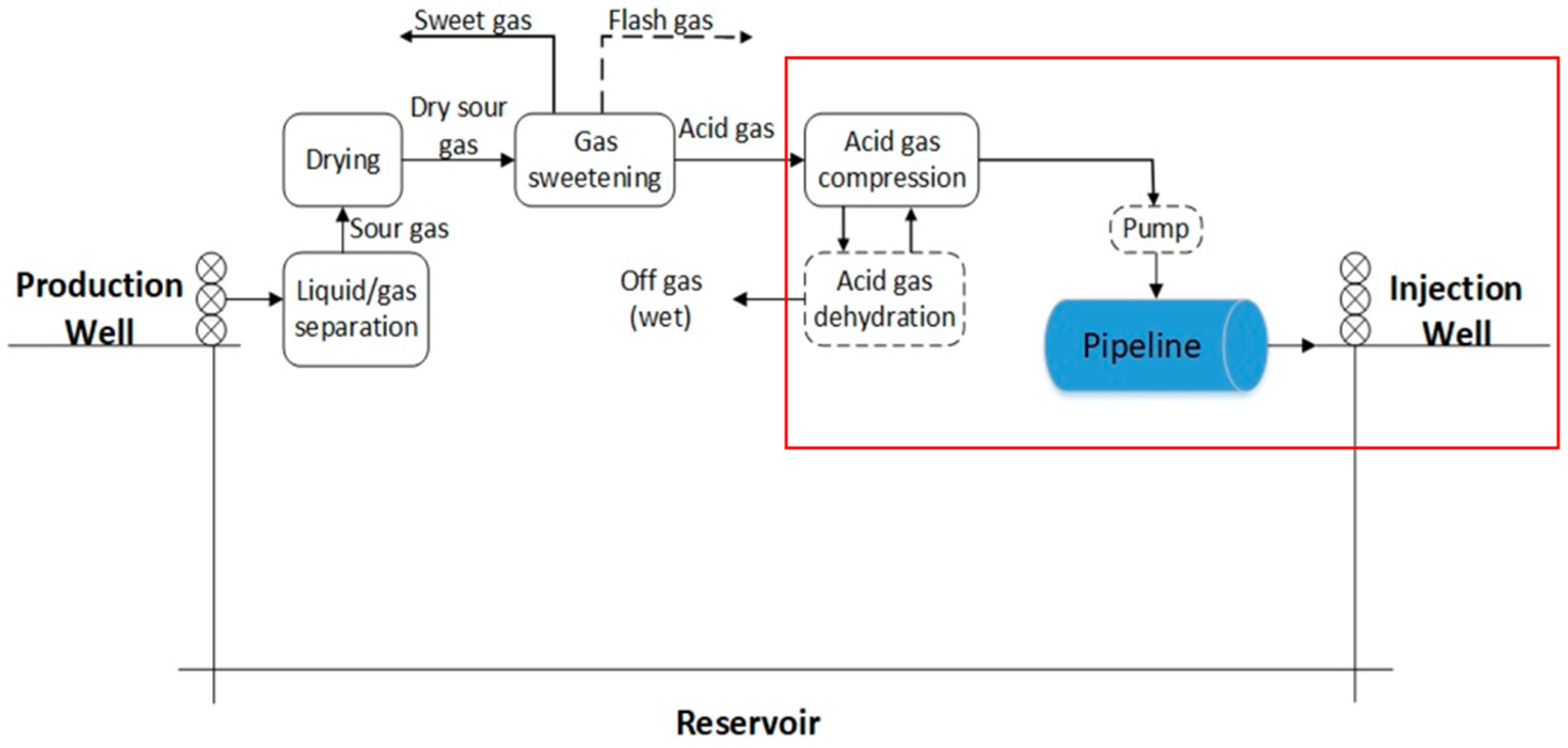
One such alternative is acid gas (re-)injection (AGI) into suitable subsurface reservoirs combining, thus cutting operating costs due to the Claus unit deactivation, reducing sulfur emissions into the atmosphere and increasing oil recovery [2,5]. In a basic AGI scheme (Figure 1), the produced reservoir gas undergoes a one- or two-stage absorbing process where it contacts an amine solution. The water-saturated acid gas mixture is then separated from the amine unit at low pressures (35 to 70 kPa) and at relatively high temperatures and is typically compressed in three or four stages to arrive at sufficiently high pressure for its injection into the subsurface formation [6,7]. The high-pressure acid gas flows through pipelines to the well site, arrives at the wellbore in a dense-fluid (liquid or supercritical) state, and finally gets injected into the reservoir through the well tubing [7]. Depending on the composition and the specifications set by the operator, it may also be necessary to dehydrate the acid gas to moderate corrosion [8].
Gas hydrates are white, solid, ice-like structures of hydrogen-bonded cavities of water molecules, in which gas molecules, H2S and CO2 in the acid gas treatment context (typically smaller than 0.9 nm), are encapsulated in the cavities of the hydrate’s crystallized cage-like lattice (Figure 2) under low temperature and elevated pressure conditions. Their structural stability depends on the van der Waals and London forces developed by the interactions between the host (water molecules) and the guest (gas molecules) components [9]. The required conditions for their formation are sufficient gas and water supply under suitable pressure and temperature conditions [10,11]. These conditions are indicated by the p-T phase envelope, also known as the hydrate equilibrium or hydrate dissociation curve which defines the boundary line below which (i.e., at lower temperatures and/or at higher pressures) hydrates might form [5].
Hydrates are considered a promising energy technology for the future as the amount of methane trapped in subsurface formations is enormous. However, they also are a long-standing challenge faced by the chemical industry when it comes to flow in pipelines and related equipment, as they are responsible for severe flow assurance issues, such as pipeline plugging, thus posing economic, safety, health and environmental risks [5,12]. When it comes to subsea or permafrost pipelines, the extreme temperature conditions prevailing in such environments severely increase the risk of hydrate formation leading to new challenges in production operations and imposing the need for additional safety control procedures [13,14]. The risk of hydrate formation can be mitigated by continuous injection of thermodynamic inhibitors, such as monoethylene glycol (MEG) [15] which causes a shift of the hydrate equilibrium curve (phase envelope) to lower temperatures and to higher pressures [16]. As this technique imposes significant additional operational costs, the accurate determination of the pressure and temperature conditions of hydrate formation using complex computational fluid dynamics (CFD) simulations becomes necessary.
Figure 2.
Molecular structure of gas hydrate [17].
Figure 2.
Molecular structure of gas hydrate [17].

For the case of sour/acid gas re-injection purposes, the hydrate formation risk is high due to the nature and prevailing conditions of this operation. Hydrates occur mostly in transportation pipelines, restrictions (chokes or valves) due to the Joule–Thompson effect, as well as at the plant restart following shut-in operations where transient conditions are observed [18]. Indeed, after the acid gas is compressed, it is directed to subsurface pipelines where the inevitably low-temperature prevailing conditions often lead to the formation of hydrates that can potentially block them. The best possible scenario would be for the acid gas to be thermally controlled sufficiently above the hydrate formation temperature and, based on the pipeline length and the seawater temperature, to arrive at the injection point (wellhead) before its temperature arrives at the formation one. Nevertheless, in cases where long pipelines must be constructed due to a large distance between the compression and the injection point, the acid gas temperature can potentially reach the temperature of the subsurface environment that, especially in deepwater and permafrost areas, can be lower than the hydrate formation one. The course of action in such cases is usually decided based on the selected surface injection design and can include a mandatory dehydration system or, if dehydration is not considered feasible due to economic, design or operating constraints, the insulation of the pipeline and its heating using electric resistances or the injection of an inhibitor (e.g., methanol) can be alternatively investigated [19].
Clearly, engineers must perform a thorough investigation on the possibility of hydrates’ appearance based on accurately predicting the hydrate formation conditions in all liable operating systems and parts to better secure the safety of the operations and, most importantly, mitigate safety, health and environmental risks. Such predictions are typically based on complex thermodynamic calculations which check for hydrates formation during the course of CFD simulations, at each segment of a pipeline network and for each timestep, for any varying composition, pressure and temperature. Millions of such calculations are needed that can become even more intense when transient, rather than steady-state conditions, are anticipated. The complexity is attributed to the use of the van der Walls–Platteeuw theory in conjunction with the Langmuir adsorption theory, further combined to quite complex fluid models to account for the polarity and electrolyte properties of the fluids phases (i.e., water and inhibitors), such as the cubic plus association (CPA) one [20]. Much more complex calculations are required to identify the exact hydrate type formed (sI or sII) [21].
To significantly accelerate such calculations, ML methods have been proposed. The concept of ML entails a set of techniques that allow the generation of computational models representing physical problems without the demand to mathematically express first principle laws. These models are developed (trained) entirely by the use of data gathered through the observation of a system and they offer explicit computational tools to understand and control the system under study [22]. Among other applications, ML methods are used to solve regression and classification problems. In the former, the model’s input is mapped to one or more continuous quantitative variables whereas in the latter, the purpose is to assign the input to one out of a number of qualitative/discrete categories (labels) [23]. In their basic form, binary classification problems assign the input to classes such as yes/no, 0/1, etc., although multiclass problems can be handled as well. During their training, classifiers learn each class’s decision boundary using ML algorithms that try to minimize the misclassification rate [24], that is, the number of data points for which a wrong class is assigned. The model development is performed using training data, which consists of several input variable samples as well as the desired output which is represented by a class for each sample (thus rendering the learning strategy as a supervised one).
As the Machine Learning (ML) community progressively expands, the number of ML-based projects has significantly increased, as evidenced by the successful implementation of several methods for a variety of engineering problems, such as for EOR-related production optimization [25,26], history matching [27,28], field development planning [29], phase behavior predictions [22,30], waterflooding processes [31], gas lift optimization [32], etc. More specifically, in the context of hydrate formation prediction and related subjects, Yu and Tian [33] developed Random Forest, Naïve Bayes and Support Vector Regression models to determine the formation conditions of natural gas hydrates. Similarly, Qasim and Lal [34] presented four different case studies involving the use of ML methods for gas hydrates prediction purposes. Suresh et al. [35] developed three ML algorithms based on Artificial Neural Networks, the Least Square version of Support Vector Machines (LSSVM), and Extremely Randomized Trees. They evaluated their accuracy in predicting gas hydrate formation conditions by using natural gas composition, pressure and inhibitor concentration as input to predict hydrate formation temperature. Finally, Kumari et al. [36] examined LSSVM and ANN models in conjunction with Genetic Programming and Genetic Algorithms to predict the stability conditions of natural gas hydrates.
In this work, a set of classifiers is proposed to handle the hydrates formation question in acid gas flow simulations. The ML models answer whether the prevailing conditions at any pipeline segment and at any timestep during the simulation lie to the left (i.e., where hydrates are formed) or to the right-hand side of the phase envelope of the fluid’s composition where hydrates formation is not favorable. Eventually, the classifiers will provide a clear answer to the hydrates formation question directly, in a non-iterative fashion, for any possible composition and prevailing conditions, in a tiny fraction of the time required by the conventional iterative, complex and CPU-demanding process. Moreover, they can account for arbitrarily high operating pressures and acid gas compositions containing various amounts of impurities and inhibitors. A large set of hydrate formation “yes/no” test points are generated offline, using the conventional, rigorous approach. Subsequently, the test data is introduced to various classifying ML architectures which are trained to provide rapidly the correct hydrate formation answer. The prediction capability and the CPU time gain of the developed tool are demonstrated by simulating the flow conditions along large pipeline networks and for a variety of acid gas compositions. The developed model is directly applicable to any acid gas pipeline problem and for any prevailing conditions to drastically reduce the CPU time spent for multiphase equilibrium calculations during heavy-duty CFD flow simulations.
The rest of the paper is structured as follows: Section 2 discusses the existing rigorous methods to determine hydrate formation conditions. In Section 3, the classification techniques tested in this study are presented, including Decision Trees, Random Forests, Support Vector Classifiers and classification Neural Networks. Additionally, this section elaborates on the methodology used for acquiring the training data. Section 4 presents a thorough analysis of the obtained results followed by an acid gas reinjection design case study. Section 6 concludes the paper with the final findings.
2. Determination of Hydrates Formation Conditions
2.1. Thermodynamic Approach
The study of hydrate phase equilibrium has a long history spanning several decades. In the 1940s, Wilcox et al. [37] developed a semi-empirical model that employed the equilibrium constants (k-values) method and relied on the theory of solid phase equilibrium to create a corresponding hydrate phase equilibrium chart. Later in 1989, Mann et al. [38] introduced an updated chart for CO2, H2S and nitrogen gas hydrates to enhance the accuracy. In 1988, Holder et al. [39] introduced the first empirical correlations for single-component gas hydrate phase equilibrium. Markogon [40] and Kobayashi et al. [41] expanded these empirical correlations to account for multiple-composition natural gas and developed correlations based on gas gravity.
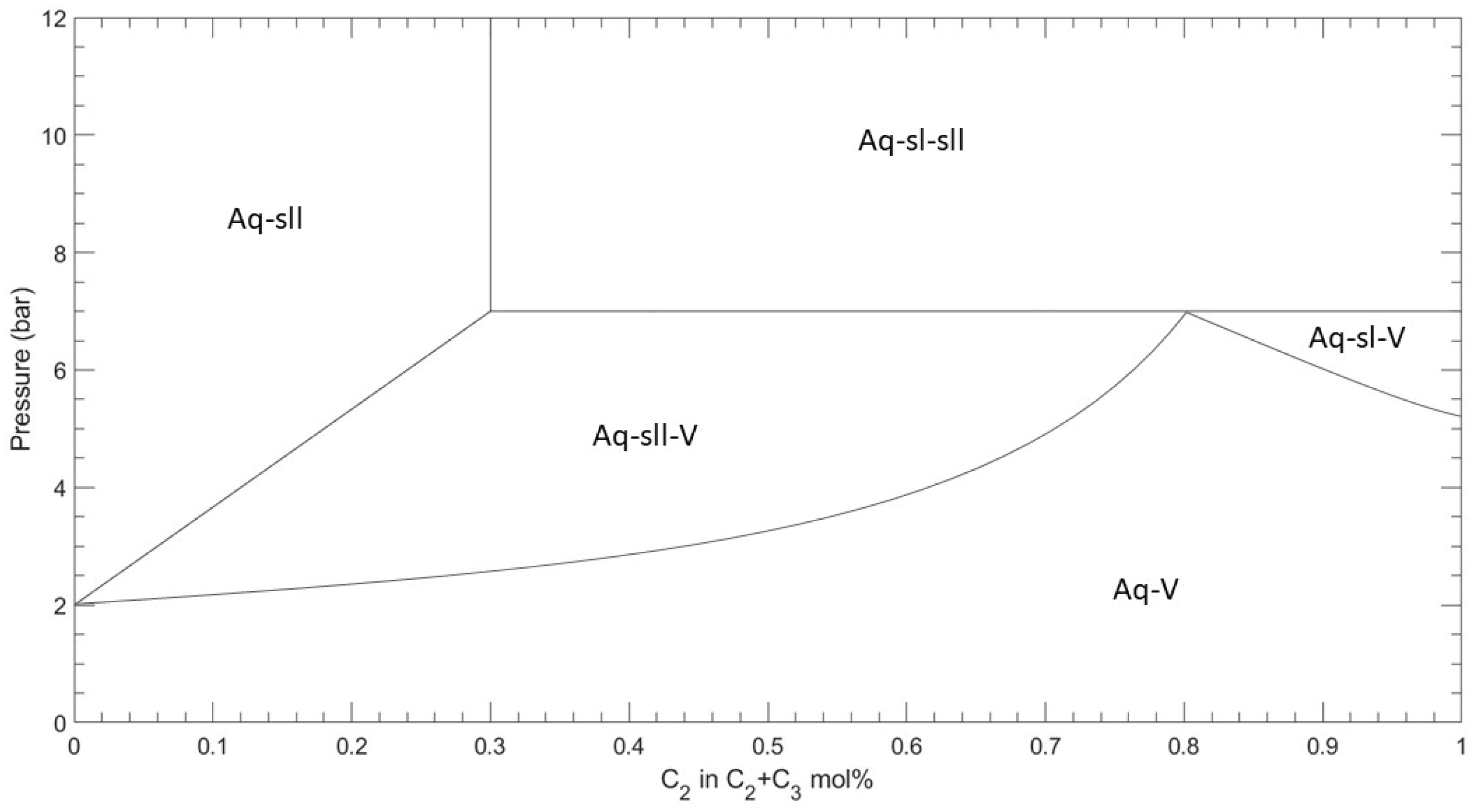
These charts and empirical correlations were extensively used in early hydrate phase equilibrium prediction but have become largely outdated with the advent of more precise rigorous thermodynamic models. Currently, the existing thermodynamic models for hydrate phase equilibrium are founded on the base model proposed by van der Waals and Platteeuw [42] as discussed below. Classic stability analysis is typically used to examine whether some specific fluid phase is formed in a mixture at given pressure and temperature conditions. When it comes to hydrates, there is no simple stability algorithm to provide a single binary answer (hydrate forming/no forming) and the presence of hydrates can only be examined by comparing the prevailing pressure (temperature) to the hydrates formation one at current temperature (pressure). This approach requires that the hydrates’ formation conditions are estimated using rigorous thermodynamic methods. Figure 3 depicts an example hydrates phase diagram formation curve for a gas mixture of C2H6 and C3H8. Various phase boundaries can be observed depending on the presence of hydrates and their specific structure type (sI or sII).
Estimating hydrates formation pressure or temperature has been a hot topic in thermodynamics since 1960 when van der Waals and Platteeuw presented the first rigorous approach. The idea lies in that at hydrate formation conditions, all phases present exhibit the same water fugacity and that hydrates appear at an infinitesimal quantity, that is
where superscripts denote hydrates, liquid, gas and ice (if applicable) phases. Therefore, estimating the formation conditions requires the solution of a multiphase phase split problem to determine the amount and composition of each phase present [44]. The computational cost to obtain the fugacity of water in the fluid phases is moderate as complex Equation of State models, such as the CPA one [20], need to be incorporated, the complexity of which is significantly higher than that of simple cubic EoS models [45]. However, the estimation of water fugacity in the hydrate phase is very cumbersome as acid gas molecules are assumed to be trapped in the water molecules’ cage through adsorption. Langmuir’s theory is utilized to describe the thermodynamics of adsorption incorporating complex potential functions such as those proposed by Kihara [46].
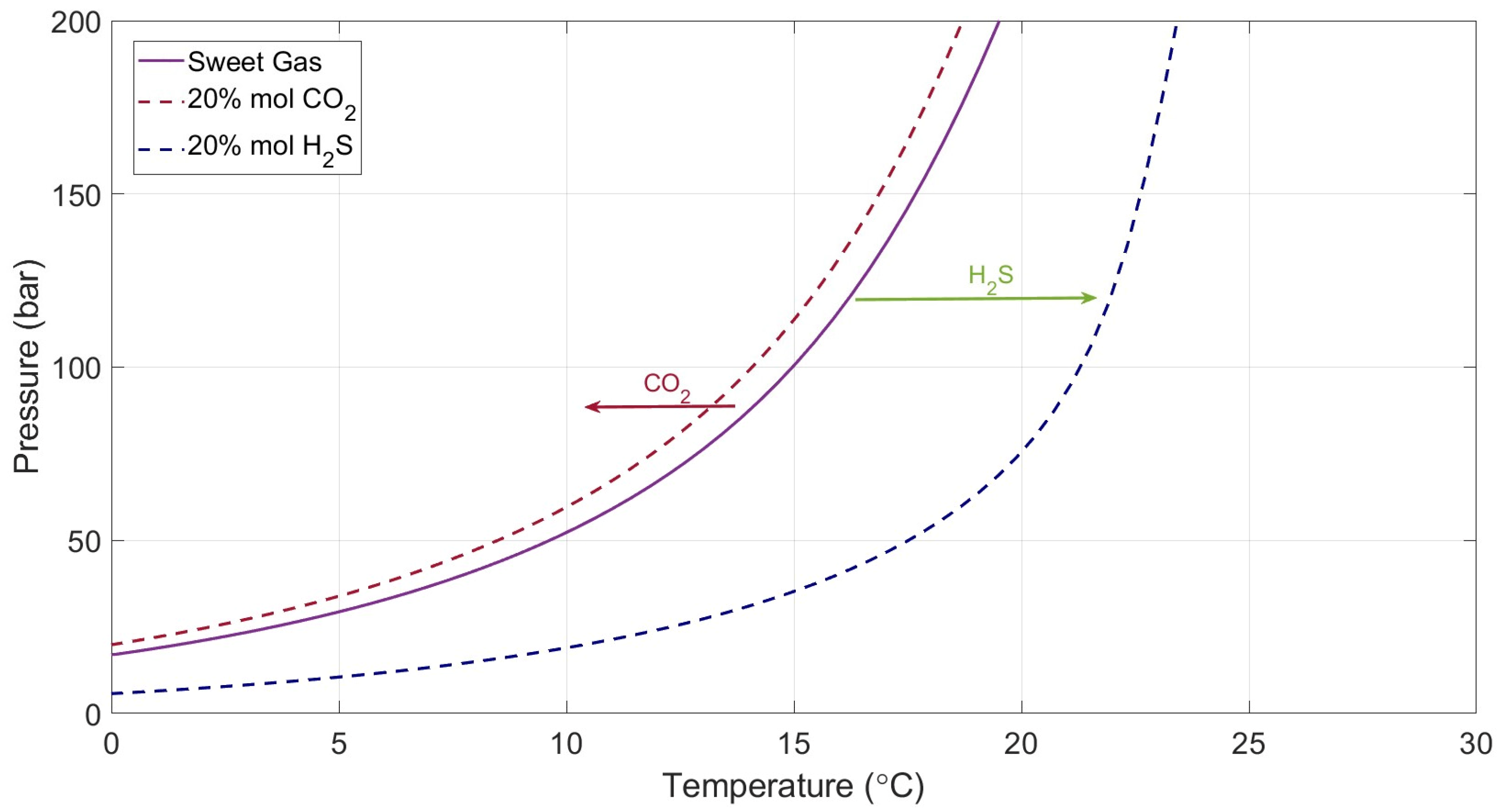
Acid gases, specifically H2S, play a significant role in altering the phase equilibrium of gas hydrates during acid gas injection operations since their presence affects both the stability and formation of hydrates. When H2S and CO2 are present in an injection system, they participate in hydrate formation along with other components and they can form hydrates at higher temperatures and lower pressures compared to methane (the dominant constituent of natural gas), thereby expanding the hydrate stability zone. In other words, the presence of these acid gases lowers the temperature and pressure thresholds for hydrate formation. Figure 4 illustrates the calculated hydrate formation curves for three different gases: a sweet gas, the sour gas obtained by enriching the sweet one with 20 mole % CO2, and 20 mole % H2S. As demonstrated, the impact of H2S is significantly more pronounced than that of CO2. While CO2 slightly depresses (shifts to the left) the hydrate formation condition, H2S considerably promotes hydrate formation [47].
Wu and Carroll [48] performed an experimental procedure to test the hydrate formation of 4 sour gas mixtures with increasing H2S content (8.3, 8.4, 11.68 and 28.8%), concluding with the following remarks:
- The hydrate formation temperature rises with an elevated H2S content and, specifically, when it exceeds 10%, there is a notable increase in the temperature of hydrate formation. For gas containing less than 10% H2S, the increase in hydrate formation temperature is relatively small, but not insignificant.
- When the gas contains more than 30% H2S, the hydrate formation temperature becomes comparable to that of pure H2S.
- The hydrate formation temperature shows a rapid increase with pressure changes at lower pressures. However, at higher pressures, the hydrate formation temperature changes more gradually, indicating that it is more sensitive to pressure variations at lower pressure levels.
The thermodynamics of hydrate formation is also influenced by the molecular size and shape of the gas. Acid gas (CO2 and H2S) have larger molecular sizes compared to methane and thus prefer to occupy larger cavities in the hydrate structure. This may lead to a change in the distribution of hydrate structures, potentially causing the hydrate to shift from a structure I (sI) to a structure II (sII) depending on the composition. Furthermore, acid gases affect the stability of the hydrate. CO2 hydrates are less stable than methane hydrates, implying that, in a mixed system, the presence of CO2 could destabilize the hydrate. However, H2S forms more stable hydrates than methane, so it can stabilize hydrates in a mixed system.
Strictly speaking, crossing the hydrates formation boundary does not necessarily mean that blockage will immediately take place. In fact, hydrates are spread in the flowing acid gas phase which is continuously enriched in solid particles, forming a “slurry”. Although the deposition, which will eventually lead to pipeline blockage, starts later, the initiation of the process acts as a warning to engineers who need to handle this issue as soon as possible.
It should be noted that this work focuses on hydrate generation rather than on hydrate blockage which requires real-time information and detailed knowledge of the exact conditions along the pipelines. Nevertheless, anticipating the blockage problem using a comparison to the phase envelope is the way engineers and related software go when first dealing with a network design problem. Steady-state network simulations are used to roughly evaluate whether hydrates endanger the acid gas flow as well as to estimate the inhibitors’ dosage, if needed. Getting further with a fully detailed analysis is not a common task, especially for small players in the market, as it requires plenty of monitoring data which will be utilized to tune and run a representative model of the flowing conditions and predict in detail hydrates blockage.
The commercial software available to the petroleum industry only handles steady-state flow conditions where time derivatives are equal to zero as is the case with Pipesim by SLB, Prosper by Petroleum Experts, HYSYS by Aspen and UniSim by Honeywell. As a result, handling the hydrates formation effect in a fully detailed level where subcooling and eventually aggregation take place needs to be handled by transient analysis. OLGA by Schlumberger and HYSYS Dynamics by Aspen are suitable products for that kind of analysis. Furthermore, according to the industry’s experience, engineers’ expertise in a corporate environment is usually focused on steady-state solutions rather than transient ones as the latter are much more complex to handle. To satisfy that need of the industry, software developers have focused mostly on steady-state products. Therefore, this work aims at providing an easy-to-embed methodology to improve the speed of exactly this kind of simulation where the only criterion that can be applied is the comparison of running conditions against the thermodynamically defined hydrate formation ones.
2.2. Classification Approach
Estimating the formation pressure (temperature) at a given temperature (pressure) is a complex task that requires multiple iterative calculations and consumes a significant part of the total acid gas flow simulation time as it involves the computation of numerous intermediate values such as components’ fugacity, Langmuir constants and cell potentials. On the other hand, the stability question eventually only requires a binary yes/no answer which, since rigorous thermodynamics cannot provide that, ML methods can be utilized instead.
Let , and correspond to the flowing stream composition and the pressure and temperature prevailing conditions. Let also denote a function that exhibits
- Positive values when the prevailing conditions do favor hydrates formation;
- Negative values when the prevailing conditions do not favor hydrates formation;
- Zero value exactly at the hydrates formation phase envelope.
Function is known as a “discriminating function”, the sign of which suffices to clearly determine the existence or not of hydrates since
To generate such a model, classification methods from the ML field, such as Decision Trees or Support Vector Machines can be utilized. The training dataset can be generated by picking random input points within the expected operating space and then running offline the rigorous hydrates stability algorithm to obtain the corresponding class label, i.e., whether hydrates are formed or not. Subsequently, the training dataset is forwarded to the training algorithm which generates the discriminating function form employing an iterative procedure known as the “training” of the classifier.
As a simple example consider a fixed acid gas composition case and a set of training points, i.e., combinations of potential pressure and temperature values. In Figure 5, points in the green-colored area correspond to conditions where hydrates formation is favorable as opposed to those in the blue background where pressure is too low or temperature is too high to allow hydrates to form. The classifier training aims at developing an explicit expression to evaluate the red line which separates the points in the two areas without allowing for misclassifications. Clearly, the more training data points, the more densely each area is populated, hence, the closer the red discriminating line lies to the exact, thermodynamically rigorous phase boundary.
3. Classification Models Development
3.1. Classification Models
Four popular ML classification techniques are evaluated in this work, namely Decision Trees (DTs), Random Forests (RFs), Support Vector Classifiers (SVCs) and classification Neural Networks (NNs). It must be emphasized that training time is not an issue in the present case, as training is performed once, offline and prior to any fluid flow simulation run. What really matters is the time required to evaluate the sign of the obtained discriminating function, i.e., obtain the label during the simulation, once the training has been completed. A very complex function expression may handicap the anticipated CPU time gain; hence, it should be dropped and replaced by another classification technique that leads to a simpler expression.
DTs construct a flowchart-like structure (Figure 6), where internal nodes represent input features such as pressure and temperature, and branches represent decision rules which split data points based on a chosen feature and threshold value (e.g., < 10 bar, > 8 °C). Finally, the ending leaf nodes represent predicted class labels (True or False). Training the DT aims at defining the appropriate order of splits, i.e., selecting the feature to be used and its splitting value, which minimizes or even zeros the misclassifications over the training population while ensuring optimal generalization capability.
To train a DT, the Gini impurity measure is utilized to select optimal splits in the variable space as a criterion that quantifies the impurity or disorder within a set of class labels. It is defined as the probability of misclassifying a randomly chosen data point based on the distribution of class labels. By selecting the splits that minimize the Gini impurity, the decision tree aims to segregate the data points into pure or nearly pure subsets, optimizing the classification accuracy. This allows the DT to effectively partition the input space based on the training data, enabling accurate predictions for new, unseen data points.
RF is an ensemble learning method that combines multiple simple DTs to create a more robust and accurate prediction model. Each tree is trained on a different subset of the data using a random subset of the input features and the algorithm randomly selects a subset of data points with replacement, a procedure known as bootstrap aggregating or “bagging”. Additionally, at each split in a DT, only a random subset of features is considered. This randomization reduces overfitting and increases the diversity among the individual DTs. The final prediction of the RF is determined by aggregating the predictions of all the individual trees through majority voting. By combining the predictions of multiple DTs, RF improves the generalization performance and provides robustness, scalability and better overall predictive accuracy compared to a single DT.
SVCs are powerful supervised ML algorithms that aim to identify an optimal hyperplane for separating data points of different classes. Unlike traditional classification algorithms that focus on minimizing misclassification error, SVMs seek to maximize the margin, which is the distance between the class discriminating hyperplane and the closest training data points, known as support vectors. The optimization task of SVMs involves finding the optimal hyperplane that maximizes the margin while correctly classifying the training data. This is achieved by solving a quadratic optimization problem subject to linear inequality constraints. To handle non-linear relationships, SVMs utilize kernel functions, such as polynomial or a Radial Basis Function (RBF), to implicitly map the input data into a higher-dimensional feature space where the data becomes linearly separable. The choice of the kernel function depends on the specific problem and the underlying characteristics of the data. By employing SVMs with appropriate kernel functions, complex decision boundaries can be captured, allowing for the effective classification of the data.
NNs are a class of ML models inspired by the structure and functioning of the human brain. They are composed of interconnected layers of artificial neurons, which are organized in an input layer, one or more hidden layers and an output one. Each neuron processes the information and passes it to the next layer through weighted connections. During the training process, NNs learn to adjust the weights of these connections based on a given objective, typically to minimize the error between the predicted and actual output. This is done through an optimization algorithm, such as gradient descent, which iteratively updates the weights to improve the network’s performance. Classification NNs obtain a class label from the output of the neural network, by applying a threshold to the value produced by the logistic function at the single output layer. The logistic function produces a value between 0 and 1, which can be interpreted as the probability of the input belonging to a particular class. By setting a threshold, typically 0.5, the input data can be assigned to class 1 if the output value is greater than or equal to the threshold, and class 0 otherwise. This way, the neural network can produce a class label based on the input data. Once trained, NNs can classify (, ) points quickly by propagating the input through the network and producing an output at the final layer.
3.2. Classification Models Input
The data required by a thermodynamically rigorous approach to determine hydrates formation conditions are the composition vector 𝐳, the prevailing pressure and temperature values as well as the component properties. The same input needs to be incorporated into the ML models apart from the component properties which are constant and do not bear any information. Based on that, the data used to train the ML models consisted of a large number of pairs, where the input vector comprises the composition vector 𝐳 containing the concentration of all four components typically found in acid gas mixtures, that is, CO2, H2S, C1 and C2. To honor the condition that the composition vector 𝐳 lies in the 3D simplex since valid composition mole fractions sum up to unity and to avoid linear dependence of the inputs, only 3 independent components concentrations were introduced, thus reducing the input vector size to 5. The pressure and temperature values for each composition combination, and , respectively, were uniformly drawn and the Prosper software by PetEx was used to construct the hydrate dissociation curves that, ultimately, generate the corresponding output vector which contains the assigned label that designates whether hydrates will form or not (1 or 0, respectively). The generated dataset can be arbitrarily large and the data itself is noise-free as it is generated by a thermodynamically consistent method such as the solids thermodynamic model implemented in the HydraFLASH software that is integrated into Prosper. For a given acid gas mixture, HydraFLASH uses the multiphase equilibrium algorithm by Michelsen [50], the van der Waals and Platteeuw theory and the CPA EoS [51] to predict the hydrate dissociation curve for the acid gas mixture of interest.
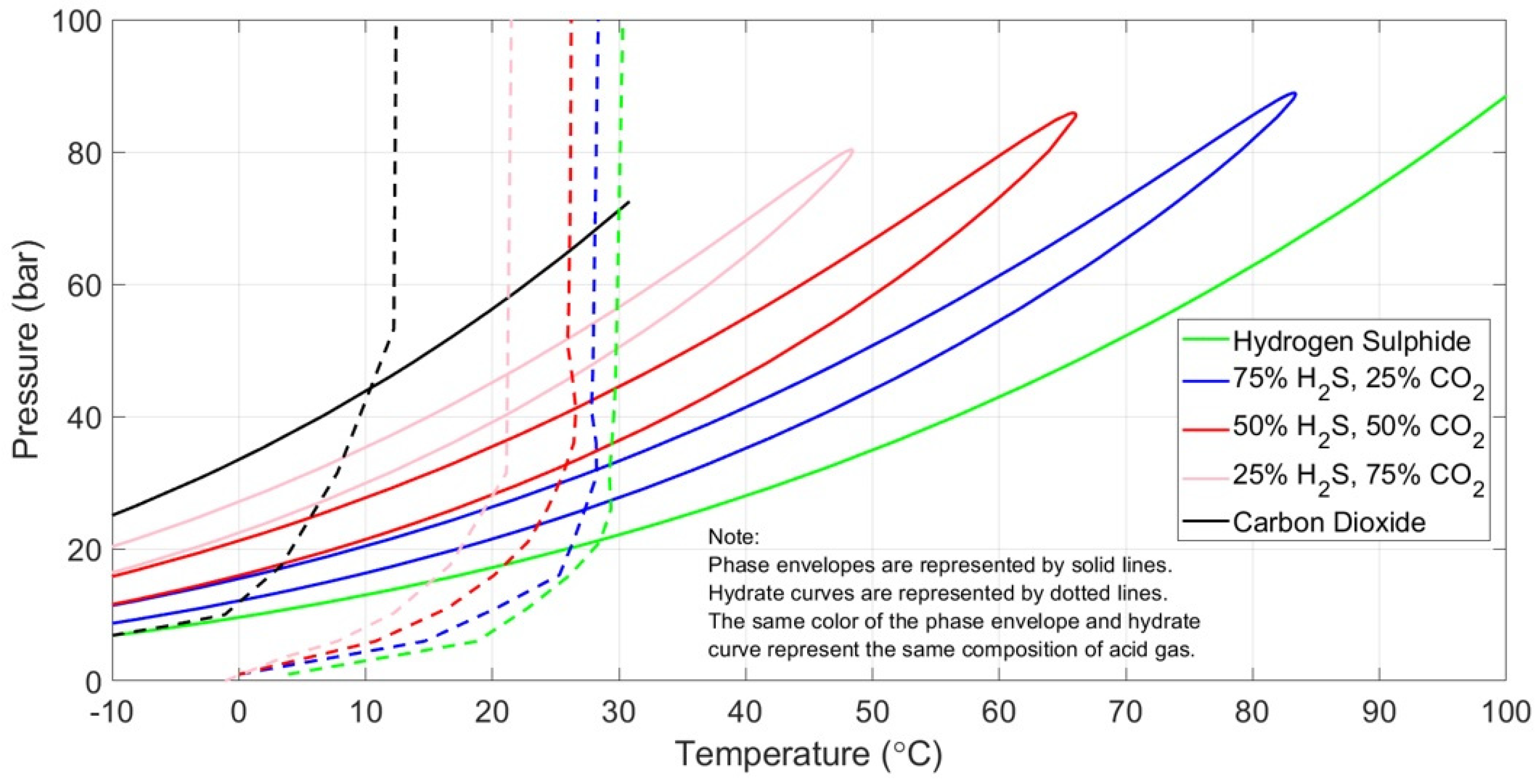
Compositions were randomly generated from the uniform distribution shown in Table 1 to densely cover the expected range of reservoir and surface conditions of the acid gas re-injection system. To account for the anticipated acid gas re-injection conditions, the pressure and temperature range of interest was determined based on the hydrate formation conditions in acid gas streams (Figure 7) as studied by Wu and Carroll [52]. This chart provides useful insight into the hydrate formation curves of three acid gas mixtures of varying H2S and CO2 content, namely 75%/25%, 50%/50% and 25%/75% with the rightmost and the leftmost lines corresponding to pure H2S and CO2, respectively. The three test acid gas mixtures lie perfectly between the two bounding curves, with decreasing maximum formation temperature as H2S decreases [5].
Based on Figure 7, the temperature range selected is [−20, 40] °C to account for the minimum possible subsea temperature (−20 °C) that may be encountered in colder regions across the world, as well as for the maximum possible upper hydrate formation temperature limit (approximately 35 °C) when a safe margin of 5 °C is added to secure a safety window (40 °C). As far as the pressure range is concerned, the lower pressure limit was dictated by the acid gas output pressure from the AU, which is close to the atmospheric one. However, the selection of the upper-pressure limit is a trickier procedure since it depends on the operation under consideration. For the case of acid/sour gas injection in shallow formations, high-pressure compressors can reach high-pressure values, up until 1000 psi (70 bar), as is the case of the high-pressurized sour gas compressor in the Tengiz field in Kazakhstan [53]. In the case of the pipeline distribution system, pressures can be as high as 2800 psi (or 190 bar) [54]. Finally, for the case of the injection pressure at the wellhead, which is determined during the process design phases and depends on the reservoir properties, it can reach values as high as 4000 psi (275 bar) [5]. Subsequently, the pressure range of [1, 300] bar was selected for the present study.
3.3. Classification Models Dataset Generation
To build the training dataset, hydrate formation curves were generated for several acid gas mixtures which span the entire composition spectrum, using the Prosper software by IPM [55]. Subsequently, for each composition, thousands of pairs were randomly generated. To properly classify the position of each test point relative to the curve (left or right), an algorithm known as the winding number algorithm was used. The winding number of a given reference point, in this case, a non-uniformly randomly generated one, is an integer that represents the total number of times that a closed curve travels counterclockwise around the point under consideration. This algorithm is implemented by, firstly, considering a horizontal line segment that starts at the reference point and extends out to positive infinity (ray). Then, the algorithm iterates over each edge of the curve and checks whether the ray cast from the point intersects the edge. If the ray intersects the edge from below and the slope of the edge is greater than the slope of the ray, the winding number is incremented otherwise it is decremented.
As the above-mentioned procedure produces uniformly drawn samples, over the operating space a tweak was used to generate a “biased” sampling procedure. Indeed, the training dataset should include more points “close” to the phase envelope, as these points provide more detailed information compared to the ones lying comfortably far to the left or right. To achieve such a non-uniform distribution of training points, each point was assigned a “keep or discard” probability as soon as it was randomly generated, which depended on its Euclidean distance to the phase boundary in the Min–Max scaled space and takes the form
The lower the distance, the higher the probability that the uniformly drawn data point will eventually be included in the training population, thus densifying points close to the phase boundary.
Ultimately, the dataset used to train the selected ML models consisted of approximately 40,000 pressure and temperature data points. A total of 60% of them were used for training purposes and another 30% for testing after the training procedure was over. Furthermore, the remaining 10% of the training dataset was retained for validation purposes to confirm the efficiency of the trained models.
4. Results
MATLAB was the commercial software utilized for the purposes of this work and all codes were developed using commands offered by the Classification Learner App contained in the Machine Learning and Deep Learning Toolbox. In-house MATLAB codes were further developed to split randomly the training dataset into training and testing points while avoiding any bias and generating extra explanatory Figures. Note that the same datasets were used to train and test all ML models.
Matlab can handle auto-tuning of model hyperparameters to identify the best set of values that result in optimal performance for a given ML model. In the case of feedforward NNs, hyperparameters include the number of hidden layers, the number of nodes in each hidden layer, and the activation functions used in the neurons, among others. A variety of optimization techniques is provided for hyperparameter tuning, such as grid search, random search, and Bayesian optimization. These methods involve searching through a predefined hyperparameter space to find the best combination that minimizes a specified objective function, such as the validation misclassification error. This can be performed using the Bayesopt function, which implements Bayesian optimization, or the OptimizeHyperparameters name–value pair with the fitensemble function, which allows for a manual specification of the hyperparameter search method.
4.1. Decision Tree Model
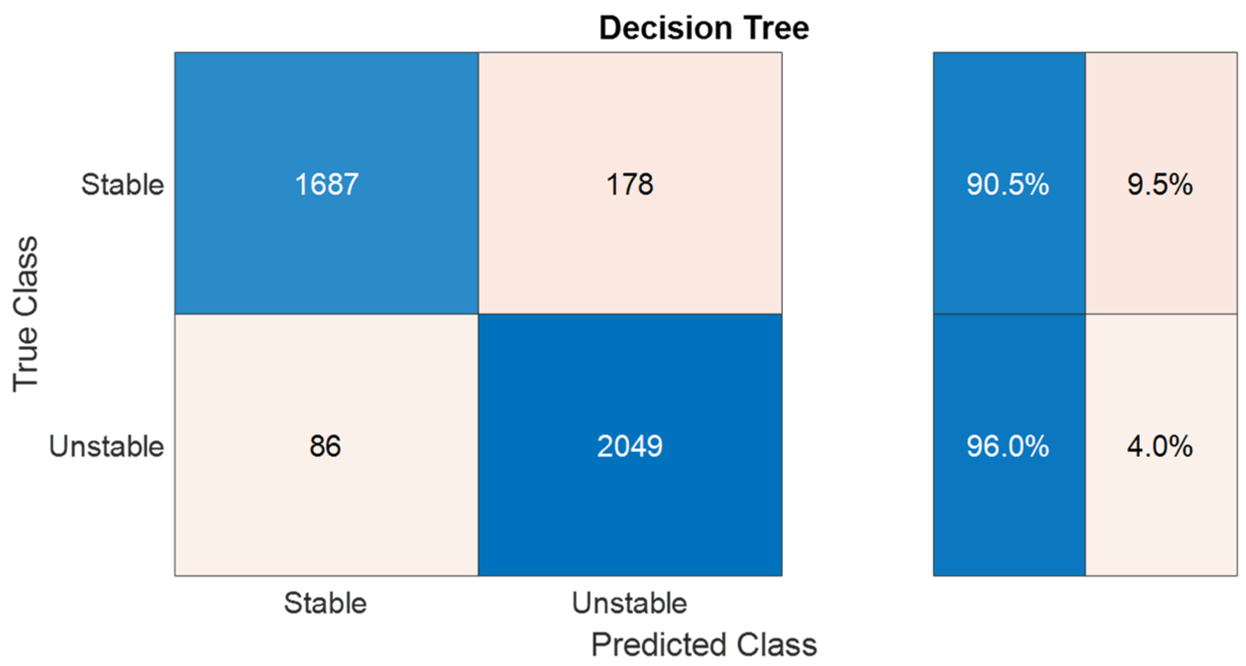
The first model to be tested is a DT model using the Gini index as the criterion for node splitting. A maximum limit of 160 splits was imposed to prevent the DT from oversizing and overfitting. To evaluate the performance of the classification model in predicting whether hydrates are formed or not, the confusion matrix of the DT, shown in Figure 8, was first evaluated. The confusion matrix rows correspond to the actual class labels, while the columns represent the predicted class labels. The cells on the main diagonal indicate correctly classified observations (shown in blue background), whereas the cells opposite to the diagonal indicate observations that were misclassified. According to Figure 8, out of the 4000 validation samples, the model accurately predicts 1687 as stable and 2049 as unstable, while incorrectly predicting 264 samples (86 + 178). As a result, false stable and false unstable predictions account for 4% and 9.5% of all stable and unstable points, respectively.
To further evaluate the classifier performance using fluid flow-oriented criteria rather than ”blind” ML-based ones, the proximity of misclassifications obtained on the validation dataset to the hydrates formation curve for two sample acid gas streams was evaluated. The first acid gas mixture is very high in H2S (97.55%), with CO2 and light hydrocarbon impurities (C1 and C2) only accounting for 2.45%. The second gas is a balanced mixture consisting of 45.18% CO2, 52.10% H2S, and 2.72% of C1 and C2. Correctly labeled points are shown in green, while false stable and false unstable answers are shown in red and blue, respectively, in Figure 9. These results demonstrate that incorrect responses for the first acid gas stream mainly occur very close to the hydrates formation curve. As a result, the impact of such a misclassification is minimal to the flow simulation given that a safety margin will be set on top of the predictions obtained. Therefore, the DT classifier is reliable, as the false stable points, which are of the utmost interest, account for a negligible proportion of the total population and are located in close proximity to the hydrate phase boundary of the acid gas mixtures under investigation.
However, the classifier does exhibit weak performance when the phase boundary shape becomes more complex, as is the case of the balanced acid gas at 27 °C and 40 bar (enclosed by a rectangle). Clearly, the classifier has missed the part which is thermodynamically related to the composition of the mixture. Nevertheless, this drawback could still be compensated by introducing a temperature “safety margin” of approximately 3 °C to the flow simulation.
4.2. Random Forest Model
As part of the investigation procedure to determine the most suitable classifier, the performance of RF models with Boosted Trees and AdaBoost, where each of the 30 DTs has a maximum limit of 100 splits imposed, was also assessed. According to Figure 10, the model performance on the validation data was significantly improved, resulting in only 2% and 3.9% of false stable and false unstable predictions, respectively. The visualization of the misclassifications for the two sample acid gas streams (Figure 11) further confirms the high reliability of the RF model employed. The RF model’s misclassifications lie even closer to the phase boundary whereas its behavior in the complex area has now been corrected. The developed RF model clearly surpasses the DT solution in terms of accuracy; however, it is worth noting that this improvement comes at the expense of increased complexity due to its ensemble nature, consisting of 30 individual DTs, in stark contrast to the simplicity of a single DT. As a result, the CPU time cost per each hydrates formation evaluation, although still a tiny fraction of the currently available rigorous thermodynamic calculation, increases by a factor of about 20 on average compared to the DT.
4.3. Support Vector Classifier
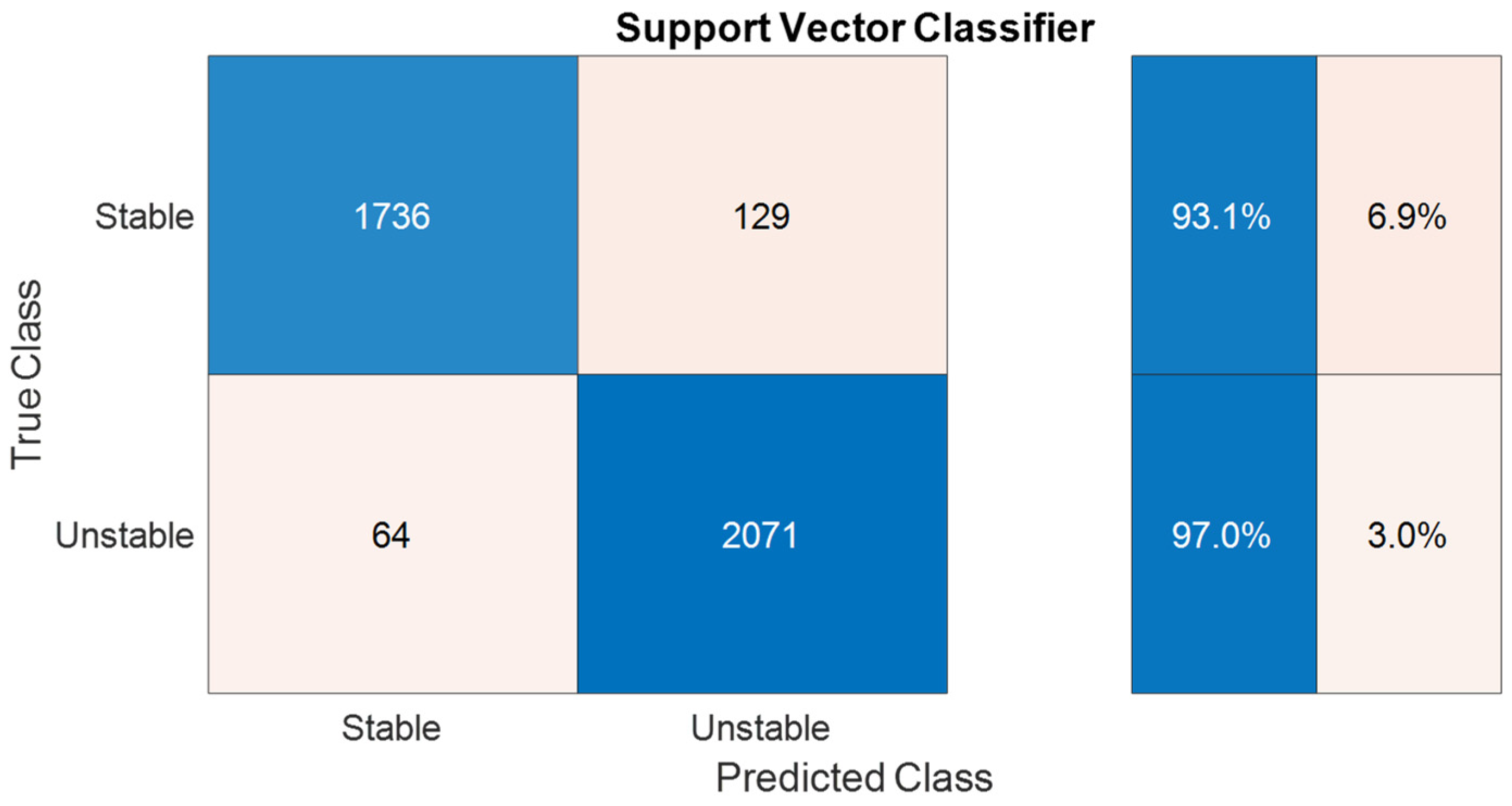
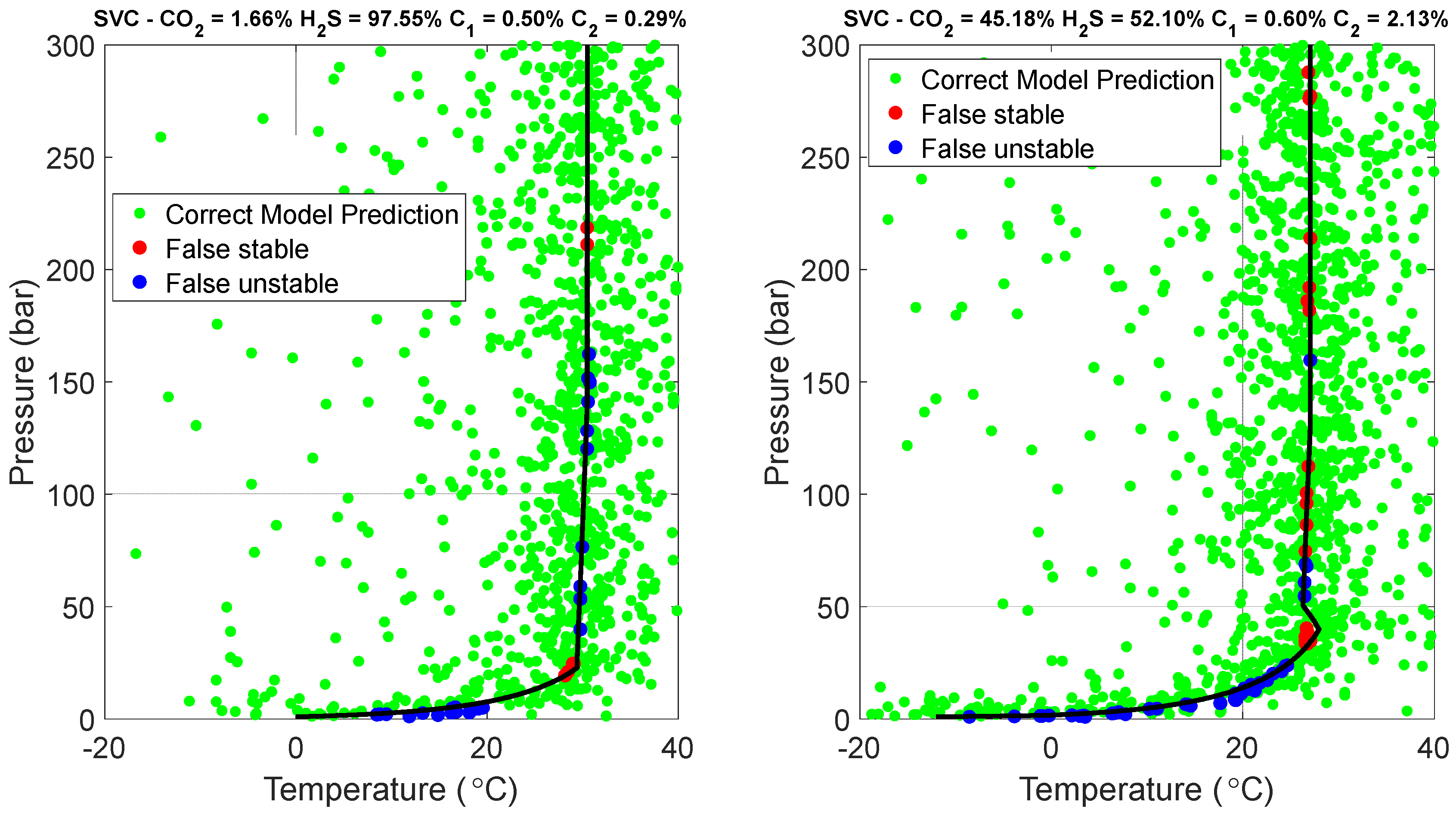
A SVC equipped with a Gaussian kernel function was also tested. SVCs, renowned for their high accuracy and robustness, are powerful ML algorithms; however, one downside to their implementation is that they are expected to be “expensive” in terms of CPU time to provide predictions on new samples due to the kernel functions involved. In this work, a total number of 5413 support vectors were identified. The results of the SVC’s assessment are presented in Figure 12, in which the confusion matrix of the Gaussian SVC shows moderate misclassification rates compared to the RF. Finally, Figure 13 illustrates the high proximity of misclassifications made by the SVC model while also showing the inability of the model to capture the complex behavior of the balanced mixture envelope. All these figures collectively indicate that SVC demonstrates enhanced reliability in accurately predicting the pressure and temperature conditions for hydrate formation but is clearly overwhelmed by the RF as far as both accuracy and CPU time requirements on new points are concerned.
4.4. Neural Network Model
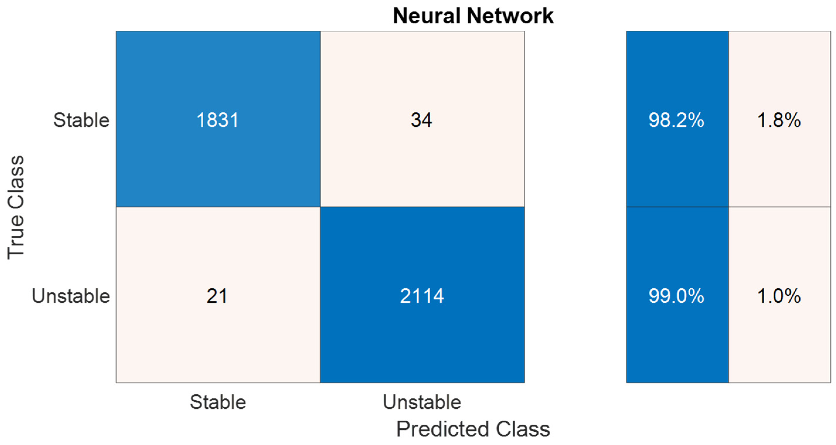
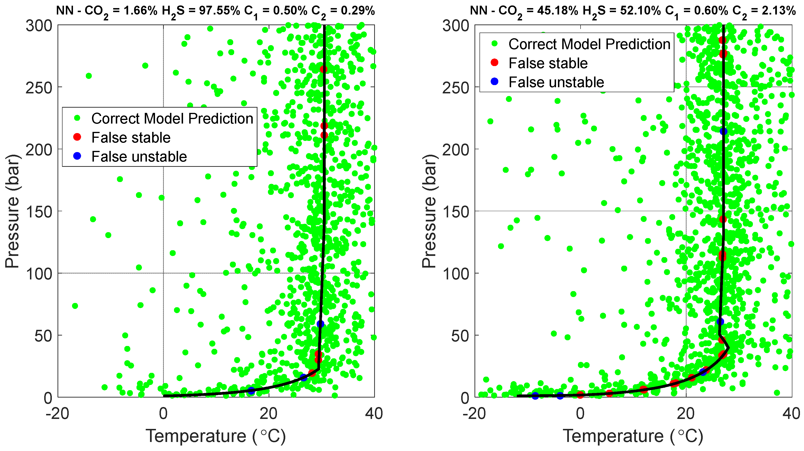
A feedforward NN was also employed, consisting of one hidden layer with 15 nodes and a logistic function applied at the single output node. Despite its reduced size, the NN outperformed any other ML model in terms of accuracy. Figure 14 illustrates that the error rate for false stable and unstable points was as low as 1% and 1.8%, respectively, resulting in an overall misclassification rate of 2.8%. Figure 15 further demonstrates that the misclassifications for the selected acid gas compositions essentially lie on the phase boundary and the complex area is handled accurately.
Table 2 provides a concise overview of the accuracy of each of the four classifiers employed.
It should be noted that the phase envelope of the quaternary mixtures studied (H2S + CO2 + C1 + C2) would exhibit a continuous shape if it had not been for its intersection with the two-phase, vapor (V)–liquid (L) envelope. As a result, the part of the hydrates phase envelope corresponding to low pressures indicates LA + V + H equilibrium, that is, the liquid aqueous phase, Vapor and Hydrate. At the point where the hydrates phase envelope intersects the low part of the two-phase boundary (such as the one shown in Figure 7), lower dew point conditions take place and two-phase acid gas equilibrium comes further into play (liquid acid gas appears), thus forming a quadruple point. Note that this is thermodynamically consistent with Gibbs law as the mixture comprises four components. The upper intersection of the hydrates phase envelope to the two-phase boundary corresponds to the conditions where vapor vanishes (bubble point), thus leaving only LA + LH + H equilibrium.
The effect of the increasing liquid acid gas (while travelling from the lower dew point to the bubble point through the two-phase envelope) to the slope of the hydrates phase boundary (i.e., what makes the difference between left- and right-hand side plots in Figure 9, Figure 11, Figure 13 and Figure 15) depends on the variety of the acid gas components concentration. The left-hand side plots correspond to compositions that are dominated by H2S (97.55%) and the two-phase boundary is too narrow to exhibit a considerable effect on the slope of the hydrates phase envelope. On the other hand, when at least two components exhibit significant concentration (as is the case with the right-hand side plots where CO2 = 45.18%, H2S = 52.10%), the change in the slope is considerable, as marked by the red rectangle.
5. Case Study
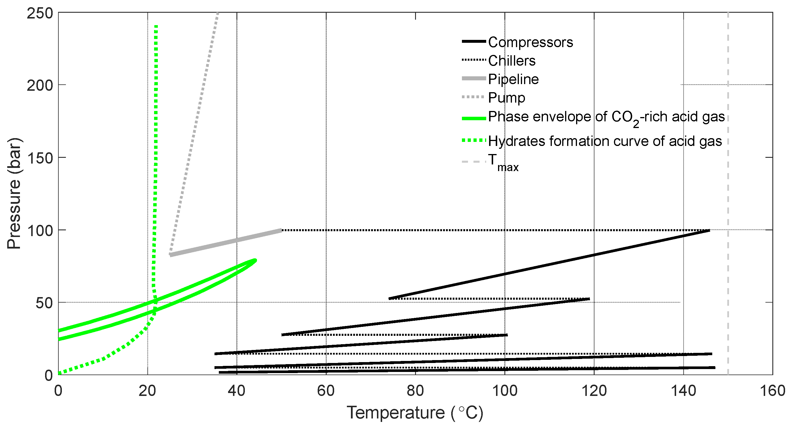
Figure 16 depicts the initially proposed design of a CO2-rich acid gas re-injection scheme. Firstly, the compressors receive the acid gas at the AU outlet and increase its pressure at a compression ratio of 2.5. Throughout each compression stage strict temperature control is maintained to ensure that the temperature of the gas exiting the compressor does not exceed 150 °C (due to the Joule–Thompson effect). Subsequently, each compression stage is followed by a cooling one (implemented using chillers) which cools down the heated fluid at constant pressure. The whole process begins at atmospheric conditions and gradually reaches a pressure of 100 bar, thus requiring a five-stage process that involves both compression and cooling of the undesired acid gas mixture produced by the reservoir. After the last cooling stage, where the acid gas turns from a supercritical fluid to a liquid, the stream is driven to the wellhead location through a subsea pipeline lying at a minimum temperature of 9 °C according to the local weather data. At that stage, the acid gas undergoes a slight pressure drop (due to friction) and a significant temperature drop due to the low temperature and huge capacity of seawater. Finally, the high pressure to ensure re-injection to the reservoir (250 bar) necessitates the inclusion of a pump.
The proposed design effectively avoids the two-phase region of the CO2-rich acid gas by developing a pressure (100 bar) higher than the acid gas cricondenbar (76 bar). However, a more thorough examination of the acid gas mixture hydrates formation curve (generated using the trained NN model and a bisection method) verifies the flow simulation results which indicate the formation of hydrates halfway along the pipeline and all along the pump path.
To remedy this situation, pipeline insulation is proposed, thus achieving a similar pressure drop but reducing the temperature drop and keeping the acid gas conditions safely away from the hydrate formation conditions (Figure 17). It should be noted that the insulation quality and thickness are also a function of the flow rate, as the lower the latter, the bigger the temperature drop since more time is allowed for the fluid to exchange heat with the seawater.
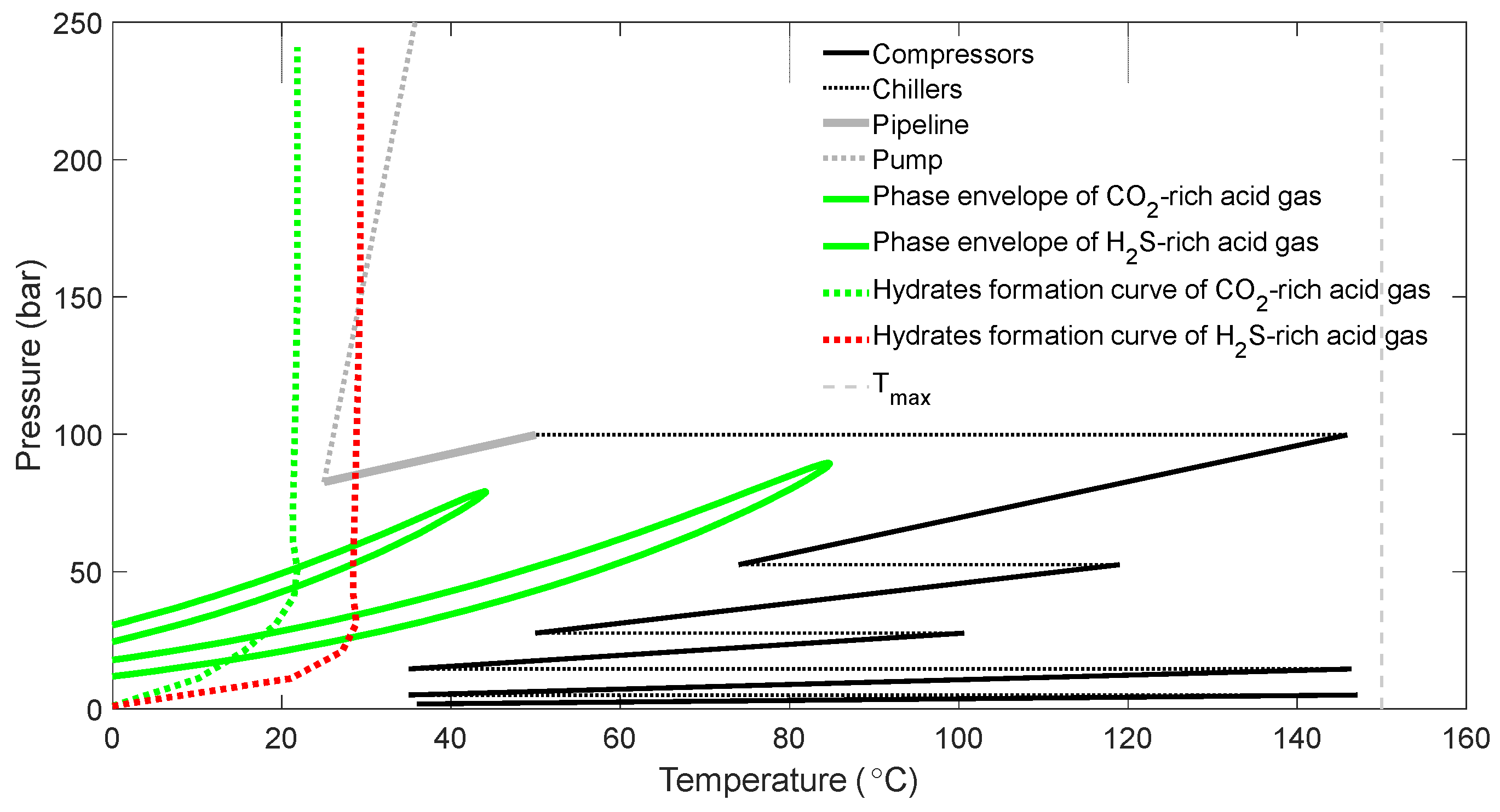
According to the operator’s field development plans, it is expected that additional H2S-rich sections of the reservoir will soon be brought into production, resulting in an increased concentration of H2S in the acid gas. This way, the design shown in Figure 17 is no longer suitable, although the prevailing conditions during compression still lie far away from the two-phase region. This is due to the shifting of the hydrates formation curve to the right-hand side by approximately 8 °C due to the increased H2S content of the acid gas stream, as shown in Figure 18. As a precautionary measure, there are two potential approaches to consider. Firstly, reinforcing the pipeline insulation can be considered to provide extra protection against hydrate formation by further reducing the temperature drop. Alternatively, the compressed gas can be mixed with some suitable additive, at a considerable cost, which helps to inhibit hydrate formation, or electric heating elements might be installed. By implementing these precautionary measures, the formation of hydrates can be successfully prevented, as demonstrated in Figure 19.
6. Conclusions
This study addresses the challenge of rapidly identifying hydrate formation in acid gas re-injection schemes in oil and gas reservoirs where millions of such calculations are required during the course of the flow simulation runs to properly design and optimize the process. Recognizing that the conventional approach of calculating hydrate formation through iterative multiphase equilibrium calculations is time-consuming and computationally intensive, this work sought a more efficient solution. A set of classifiers was developed to quickly determine the likelihood of hydrate formation given the prevailing pressure and temperature conditions, as well as the composition of flowing acid gas mixtures. These classifiers offer a direct, non-iterative approach, bypassing the need for lengthy calculations and reducing by orders of magnitude the computational time required for multiphase equilibrium analysis. In order to train the classifiers and ensure accurate predictions, a large dataset of hydrate formation data was generated offline using traditional methods.
The results of the study demonstrated the effectiveness and high precision of the classifiers in predicting hydrate formation. Among the classifiers tested, the NN classifier exhibited the highest accuracy in detecting hydrate formation, providing reliable insights into the occurrence of hydrates. The DTs classifier emerged as the fastest option, enabling rapid assessments in real-time scenarios at the cost of reduced accuracy. By enabling rapid and reliable predictions, the trained classifiers can help operators minimize operational costs, comply with air emission standards, and optimize the flow scheme. The ability to identify hydrate formation potential in an infinitesimal fraction of the time required by conventional methods can greatly improve operational efficiency and decision making in acid gas injection processes.
The potential impact of this study on future research and applications is substantial. The development of classifiers for hydrate formation prediction opens up possibilities for further advancements in fluid flow simulations and computational modeling in the chemical industry. By reducing the computational time required for multiphase equilibrium calculations, this research paves the way for a more efficient and accurate analysis of hydrate-related issues in acid gas pipelines. Future studies can build upon this work to refine the classifiers and explore additional applications to address more challenges in the industry.
Author Contributions
Conceptualization, A.S. and V.G.; methodology, A.S., E.M.K. and S.P.F.; software, A.S., E.M.K. and S.P.F.; validation, V.G.; writing—original draft preparation, A.S., E.M.K. and S.P.F.; writing—review and editing, V.G.; visualization, E.M.K.; supervision, V.G. All authors have read and agreed to the published version of the manuscript.
Funding
This research received no external funding.
Data Availability Statement
No public or private data where used or analyzed in this study. The data used were generated by commercial software, thus data sharing is not applicable.
Conflicts of Interest
The authors declare no conflict of interest.
References
- Siddiqui, M.I.; Baber, S.; Saleem, W.A.; Jafri, M.O.; Hafeez, Q. Industry practices of sour gas management by reinjection: Benefits, methodologies, economic evaluation and case studies. In Proceedings of the SPE/PAPG Annual Technical Conference, Islamabad, Pakistan, 26–27 November 2013; p. SPE-169645-MS. [Google Scholar]
- Kokal, S.L.; Al-Utaibi, A. Sulfur Disposal by Acid Gas Injection: A Road Map and A Feasibility Study. In Proceedings of the SPE Middle East Oil and Gas Show and Conference, Al Manama, Bahrain, 12–15 March 2005; p. SPE-93387-MS. [Google Scholar]
- Maddocks, J. Capacity Control Considerations for Acid Gas Injection Systems; Gas Liquids Engineering Ltd.: Calgary, AB, Canada, 2015. [Google Scholar]
- Burgers, W.F.J.; Northrop, P.S.; Kheshgi, H.S.; Valencia, J.A. Worldwide development potential for sour gas. Energy Procedia 2011, 4, 2178–2184. [Google Scholar] [CrossRef] [Green Version]
- Samnioti, A.; Kanakaki, E.M.; Koffa, E.; Dimitrellou, I.; Tomos, C.; Kiomourtzi, P.; Gaganis, V.; Stamataki, S. Wellbore and reservoir thermodynamic appraisal in acid gas injection for EOR operations. Energies 2023, 16, 2392. [Google Scholar] [CrossRef]
- Bachu, S.; Gunter, W.D. Overview of acid-gas injection operations in Western Canada. In Proceedings of the 7th International Conference on Greenhouse Gas Control Technologies, Vancouver, BC, Canada, 5 September 2004. [Google Scholar]
- Mokhatab, S.; Poe, W.A.; Mak, J.W. Handbook of Natural Gas Transmission and Processing, 4th ed.; Gulf Professional Publishing: Cambridge, MA, USA, 2019; ISBN 978-0-12-815817-3. [Google Scholar]
- Carroll, J.J. Acid gas injection: Past, present, and future. In Proceedings of the International Acid Gas Injection Symposium, Calgary, AB, Canada, 5–6 October 2009. [Google Scholar]
- Ismail, I.; Gaganis, V.; Marinakis, D.; Mousavi, R.; Tohidi, B. Accuracy of different thermodynamic software packages in predicting hydrate dissociation conditions. Chem. Thermodyn. Therm. Anal. 2023, 9, 100103. [Google Scholar] [CrossRef]
- Zatsepina, O.; Buffett, B.A. Thermodynamic conditions for the stability of gas hydrate in the seafloor. J. Geophys. Res. 1998, 103, 24127–24139. [Google Scholar] [CrossRef]
- Davidson, D.W.; Garg, S.K.; Gough, S.R.; Handa, Y.; Ratcliffe, C.I.; Ripmeester, J.; Tse, J.; Lawson, W.F. Laboratory analysis of a naturally occurring gas hydrate from sediment of the Gulf of Mexico. Geochim. Cosmochim. Acta 1986, 50, 619–623. [Google Scholar] [CrossRef]
- Chatti, I.; Delahaye, A.; Fournaison, L. Benefits and drawbacks of clathrate hydrates: A review of their areas of interest. Energy Convers. Manag. 2005, 46, 1333–1343. [Google Scholar] [CrossRef]
- Sharma, S.; Saxena, A.; Saxena, N. Challenges in Gas Hydrate Formation in Oil Industry. In Unconventional Resources in India: The Way Ahead; Springer: Cham, Switzerland, 2019; ISBN 978-3-030-21413-5. [Google Scholar]
- Barker, J.; Gomez, R. Formation of Hydrates During Deepwater Drilling Operation. J. Pet. Technol. 1989, 41, 297–301. [Google Scholar] [CrossRef]
- Bharathi, A.; Nashed, O.; Lal, B.; Foo, K.S. Experimental and modeling studies on enhancing the thermodynamic hydrate inhibition performance of monoethylene glycol via synergistic green material. Sci. Rep. 2021, 11, 2396. [Google Scholar] [CrossRef]
- Kim, J.; Kim, H.; Sohn, Y.; Chang, D.; Seo, Y.; Kang, S.P. Prevention of methane hydrate reformation in transport pipeline using thermodynamic and kinetic hydrate inhibitors. J. Pet. Sci. Eng. 2017, 154, 114–125. [Google Scholar] [CrossRef]
- Managing Impacts of Deep Sea Resource Exploitation. Methane from Marine Gas Hydrates. Available online: https://www.eumidas.net/sites/default/files/downloads/Briefs/MIDAS_hydrates_brief_lowres.pdf (accessed on 17 May 2023).
- Hajiw, M. Hydrate Mitigation in Sour and Acid Gases. In Chemical and Process Engineering; Ecole Nationale Supérieure des Mines de Paris: Paris, France, 2014. [Google Scholar]
- Grynia, E.W.; Carroll, J.J.; Griffin, P.J. Dehydration of acid gas prior to injection. In Proceedings of the 2nd Annual Gas Processing Symposium, Doha, Qatar, 10–14 January 2010; pp. 177–185. [Google Scholar]
- Kontogeorgis, G.M.; Voutsas, E.C.; Yakoumis, I.V.; Tassios, D.P. An equation of state for associating fluids. Ind. Eng. Chem. Res. 1996, 35, 4310–4318. [Google Scholar] [CrossRef]
- Sloan, E.D. Fundamental principles and applications of natural gas hydrates. Nature 2003, 426, 353–359. [Google Scholar] [CrossRef]
- Samnioti, A.; Anastasiadou, V.; Gaganis, V. Application of machine learning to accelerate gas condensate reservoir simulation. Clean Technol. 2022, 4, 153–173. [Google Scholar] [CrossRef]
- Bishop, C.M. Pattern Recognition and Machine Learning, 1st ed.; Springer: New York, NY, USA, 2006; ISBN 978-0-387-31073-2. [Google Scholar]
- Nocedal, J.; Wright, S. Numerical Optimization, 2nd ed.; Mikosch, T.V., Robinson, S.M., Resnick, S.I., Eds.; Springer: New York, NY, USA, 2006; ISBN 0-387-30303-0. [Google Scholar]
- Thanh, H.V.; Sugai, Y.; Sasaki, K. Application of artificial neural network for predicting the performance of CO2 enhanced oil recovery and storage in residual oil zones. Sci. Rep. 2020, 10, 18204. [Google Scholar] [CrossRef]
- Ampomah, W.; Balch, R.S.; Cather, M.; Will, R.; Gunda, D.; Dai, Z.; Soltanian, M.R. Optimum design of CO2 storage and oil recovery under geological uncertainty. Appl. Energy 2017, 195, 80–92. [Google Scholar] [CrossRef]
- Sampaio, T.P.; Ferreira Filho, V.J.M.; de Sa Neto, A. An Application of Feed Forward Neural Network as Nonlinear Proxies for the Use During the History Matching Phase. In Proceedings of the Latin American and Caribbean Petroleum Engineering Conference, Cartagena de Indias, Colombia, 30–31 May 2009; p. SPE-122148-MS. [Google Scholar]
- Ramgulam, A.; Ertekin, T.; Flemings, P.B. Utilization of Artificial Neural Networks in the Optimization of History Matching. In Proceedings of the Latin American & Caribbean Petroleum Engineering Conference, Buenos Aires, Argentina, 15–18 April 2007; p. SPE-107468-MS. [Google Scholar]
- Avansi, G.D. Use of Proxy Models in the Selection of Production Strategy and Economic Evaluation of Petroleum Fields. In Proceedings of the SPE Annual Technical Conference and Exhibition, New Orleans, LA, USA, 4–7 October 2009; p. SPE-129512-STU. [Google Scholar]
- Anastasiadou, V.; Samnioti, A.; Kanakaki, R.; Gaganis, V. Acid gas re-injection system design using machine learning. Clean Technol. 2022, 4, 1001–1019. [Google Scholar] [CrossRef]
- Zhong, Z.; Sun, A.Y.; Wang, Y.; Ren, B. Predicting field production rates for waterflooding using a machine learning-based proxy model. J. Pet. Sci. Eng. 2020, 194, 107574. [Google Scholar] [CrossRef]
- Ebrahimi, A.; Khamehchi, E. Developing a novel workflow for natural gas lift optimization using advanced support vector machine. J. Nat. Gas Sci. Eng. 2016, 28, 626–638. [Google Scholar] [CrossRef]
- Yu, Z.; Tian, H. Application of Machine Learning in Predicting Formation Condition of Multi-Gas Hydrate. Energies 2022, 15, 4719. [Google Scholar] [CrossRef]
- Qasim, A.; Lal, B. Machine Learning Application in Gas Hydrates. In Machine Learning and Flow Assurance in Oil and Gas Production; Springer: Cham, Switzerland, 2019; ISBN 978-3-031-24230-4. [Google Scholar]
- Suresh, S.D.; Lal, B.; Qasim, A.; Foo, K.S.; Sundramoorthy, J.D. Application of Machine Learning Models in Gas Hydrate Mitigation. In Proceedings of the International Conference on Artificial Intelligence for Smart Community, Universiti Teknologi Petronas, Seri Iskandar, Malaysia, 17–18 December 2020. [Google Scholar]
- Kumari, A.; Madhaw, M.; Pendyala, V.S. Prediction of Formation Conditions of Gas Hydrates Using Machine Learning and Genetic Programming. In Machine Learning for Societal Improvement, Modernization, and Progress; IGI Global: Hershey, PA, USA, 2022; ISBN 1668440458. [Google Scholar]
- Wilcox, W.I.; Carson, D.B.; Katz, D.L. Natural Gas Hydrates. Ind. Eng. Chem. 1941, 33, 662–665. [Google Scholar] [CrossRef]
- Mann, S.L.; McClure, L.M.; Poettmann, F.H.; Sloan, E.D. Vapor-Solid Equilibrium Ratios for Structure I and II Natural Gas Hydrates. In Proceedings of the 68th GPA Annual Convention, San Antonio, TX, USA, 13–14 March 1989. [Google Scholar]
- Holder, G.D.; Zetts, S.P.; Pradhan, N. Phase Behavior in Systems Containing Clathrate Hydrates. Rev. Chem. Eng. 1988, 5, 1–70. [Google Scholar] [CrossRef]
- Markogon, F.Y. Hydrates of Natural Gas; PennWell Books: Tulsa, OK, USA, 1981; ISBN 0878141650. [Google Scholar]
- Kobayashi, B.R.; Kyoo, Y.S.; Sloan, E.D. Phase Behavior of Water/Hydrocarbon Systems. In Petroleum Handbook; SPE: Richardson, TX, USA, 1987; pp. 13–25. [Google Scholar]
- Platteeuw, J.C.; van der Waals, J.H. Thermodynamics Properties of Gas Hydrates. Mol. Phys. 1958, 1, 91–96. [Google Scholar] [CrossRef]
- Sloan, E.D., Jr.; Koh, C.A.; Koh, C.A. Clathrate Hydrates of Natural Gases, 3rd ed.; CRC Press: Boca Raton, FL, USA, 2007. [Google Scholar]
- Michelsen, M.L. The isothermal flash problem. Part II: Phase-split calculation. Fluid Phase Equilibria 1982, 9, 21–40. [Google Scholar] [CrossRef]
- Privat, R.; Jaubert, J.N. Thermodynamic models for the prediction of petroleum-fluid phase behaviour. In Crude Oil Emulsions-Composition Stability and Characterization; Intechopen: London, UK, 2019; ISBN 978-953-51-0220-5. [Google Scholar]
- Kihara, T. The Second Virial Coefficient of Non-Spherical Molecules. J. Phys. Soc. Jpn. 1951, 6, 289–296. [Google Scholar] [CrossRef]
- Campbell, J.M. Sour Gas Hydrate Formation Phase Behavior. Available online: http://www.jmcampbell.com/tip-of-the-month/2012/12/sour-gas-hydrate-formation-phase-behavior/ (accessed on 26 July 2023).
- Wu, Y.; Carroll, J.J. Acid Gas Injection and Related Technologies; Scrivener Publishing LLC: Beverly, MA, USA, 2011; ISBN 9781118094273. [Google Scholar]
- Cavaioni, M. Machine Learning: Decision Tree Classifier. Medium. Available online: https://medium.com/machine-learning-bites/machine-learning-decision-tree-classifier-9eb67cad263e (accessed on 17 June 2013).
- Michelsen, M.L. Multiphase isenthalpic and isentropic flash algorithms. Fluid Phase Equilibria 1987, 33, 13–27. [Google Scholar] [CrossRef]
- Palma, A.M.; Queimada, A.J.; Coutinho, J. Modelling Hydrate Dissociation Curves in the presence of hydrate inhibitors with a modified CPA EoS. Ind. Eng. Chem. Res. 2019, 58, 19239–19250. [Google Scholar] [CrossRef]
- Wu, Y.; Carroll, J.J. The research on experiments and theories about hydrates in high-sulfur gas reservoirs. In Acid Gas Injection and Related Technologies; Wiley: Hoboken, NJ, USA, 2011; ISBN 978-1-118-09426-6. [Google Scholar]
- Darmentaev, S.; Yessaliyeva, A.; Azhigaliyeva, A.; Belanger, D.; Sullivan, M.; King, G.; Feyijimi, T.; Bateman, P. Tengiz Sour Gas Injection Project. In Proceedings of the SPE Caspian Carbonates Conference, Atyrau, Kazakhstan, 8–10 November 2010; p. SPE 139851. [Google Scholar]
- Energy Equipment and Infrastructure Alliance. Meeting the Dual Challenge: A Roadmap to at-Scale Deployment of Carbon Capture, Use and Storage. Volume III, Chapter 6: CO2 Transport. 2019. Available online: https://www.eeia.org/post/CCUS-Pipeline-Transport-Meeting-the-Dual-Challenge.pdf (accessed on 10 June 2023).
- Prosper Software User Manual, Version 12; Petroleum Experts Ltd.: Edinburgh, UK, 2013.
Figure 1.
Acid gas treatment and re-injection process [5].
Figure 1.
Acid gas treatment and re-injection process [5].

Figure 3.
Example hydrates formation curve, Reproduced from [43].
Figure 3.
Example hydrates formation curve, Reproduced from [43].

Figure 4.
Sweet gas (purple line), CO2 (red dashed line) and H2S (blue dashed line) enriched gas dissociation curves [47].
Figure 4.
Sweet gas (purple line), CO2 (red dashed line) and H2S (blue dashed line) enriched gas dissociation curves [47].

Figure 5.
Hydrates formation envelope.

Figure 6.
Decision Tree with 4 inputs (x, y, z, w) and 6 splits [49].
Figure 6.
Decision Tree with 4 inputs (x, y, z, w) and 6 splits [49].

Figure 7.
Hydrates formation curves for various acid gas compositions.

Figure 8.
DT confusion matrix on validation data.

Figure 9.
Visualization of the DT model on training data points.

Figure 10.
RF confusion matrix on validation data.

Figure 11.
Visualization of the RF model on training data points.

Figure 12.
SVC confusion matrix on validation data.

Figure 13.
Visualization of the SVC model on training data points.

Figure 14.
NN confusion matrix on validation data.

Figure 15.
Visualization of the NN model on training data points.

Figure 16.
Initial design of the CO2-rich acid gas re-injection scheme.

Figure 17.
Enhanced design of the CO2-rich acid gas re-injection scheme.

Figure 18.
Initial design of the H2S-rich acid gas re-injection scheme.

Figure 19.
Enhanced design of the H2S-rich acid gas re-injection scheme.


Table 1.
Range of acid gas mixture components concentration.
| Component | Range (mol%) |
|---|---|
| H2S | 1–99% |
| CO2 | 1–99% |
| C1 | 0–5% |
| C2 | 0–3% |
Table 2.
Range of acid gas mixture components concentration.
| Classifier | Classifier Type | Accuracy (%) |
|---|---|---|
| Decision Trees | Fine Tree | 93.9 |
| Ensemble Classifiers | Boosted Trees | 97.4 |
| Support Vector Classifiers | Gaussian | 95.5 |
| Neural Network Classifiers | Neural Networks | 98.6 |
Disclaimer/Publisher’s Note: The statements, opinions and data contained in all publications are solely those of the individual author(s) and contributor(s) and not of MDPI and/or the editor(s). MDPI and/or the editor(s) disclaim responsibility for any injury to people or property resulting from any ideas, methods, instructions or products referred to in the content. |
© 2023 by the authors. Licensee MDPI, Basel, Switzerland. This article is an open access article distributed under the terms and conditions of the Creative Commons Attribution (CC BY) license (https://creativecommons.org/licenses/by/4.0/).
Share and Cite
MDPI and ACS Style
Samnioti, A.; Kanakaki, E.M.; Fotias, S.P.; Gaganis, V. Rapid Hydrate Formation Conditions Prediction in Acid Gas Streams. Fluids 2023, 8, 226. https://doi.org/10.3390/fluids8080226
AMA Style
Samnioti A, Kanakaki EM, Fotias SP, Gaganis V. Rapid Hydrate Formation Conditions Prediction in Acid Gas Streams. Fluids. 2023; 8(8):226. https://doi.org/10.3390/fluids8080226
Chicago/Turabian StyleSamnioti, Anna, Eirini Maria Kanakaki, Sofianos Panagiotis Fotias, and Vassilis Gaganis. 2023. "Rapid Hydrate Formation Conditions Prediction in Acid Gas Streams" Fluids 8, no. 8: 226. https://doi.org/10.3390/fluids8080226