
Prediction of Biochar Yield and Specific Surface Area Based on Integrated Learning Algorithm
by

Xiaohu Zhou
1,
Xiaochen Liu
1,2,*,
Linlin Sun
1,
Xinyu Jia
1,
Fei Tian
1,
Yueqin Liu
3 and
Zhansheng Wu
1,* 1
Xi’an Key Laboratory of Textile Chemical Engineering Auxiliaries, School of Environmental and Chemical Engineering, Xi’an Polytechnic University, Xi’an 710048, China
2
Shaanxi Key Laboratory of Degradable Biomedical Materials, School of Chemical Engineering, Northwest University, Xi’an 710069, China
3
School of Life Science, Yan’an University, Yan’an 716000, China
*
Authors to whom correspondence should be addressed.
C 2024, 10(1), 10; https://doi.org/10.3390/c10010010
Submission received: 20 November 2023
/
Revised: 2 January 2024
/
Accepted: 7 January 2024
/
Published: 12 January 2024
Abstract
:Biochar is a biomaterial obtained by pyrolysis with high porosity and high specific surface area (SSA), which is widely used in several fields. The yield of biochar has an important effect on production cost and utilization efficiency, while SSA plays a key role in adsorption, catalysis, and pollutant removal. The preparation of biochar materials with better SSA is currently one of the frontiers in this research field. However, traditional methods are time consuming and laborious, so this paper developed a machine learning model to predict and study the properties of biochar efficiently for engineering through cross-validation and hyper parameter tuning. This paper used 622 data samples to predict the yield and SSA of biochar and selected eXtreme Gradient Boosting (XGBoost) as the model due to its excellent performance in terms of performance (yield correlation coefficient R2 = 0.79 and SSA correlation coefficient R2 = 0.92) and analyzed it using Shapley Additive Explanation. Using the Pearson correlation coefficient matrix revealed the correlations between the input parameters and the biochar yield and SSA. Results showed the important features affecting biochar yield were temperature and biomass feedstock, while the important features affecting SSA were ash and retention time. The XGBoost model developed provides new application scenarios and ideas for predicting biochar yield and SSA in response to the characteristic input parameters of biochar.
1. Introduction
In the face of the dual pressures of growing energy demand and environmental pollution caused by fossil fuels on a global scale, biomass has attracted much attention as one of the most abundant and promising renewable materials [1]. The annual global biomass production is about 101.1 billion tons [2]. However, most of the biomass resources exist in the form of waste, such as agricultural straw [3] and building materials’ wood chips [4]. The treatment of these biomass wastes is often time consuming and laborious, which not only increases energy consumption but also pollutes the environment again by improper treatment. How to utilize these biomass resources effectively is an important topic that scientists worldwide have been trying to study [5]. At present, the idea of using these biomass wastes to prepare biochar is one of the most effective means to solve this problem. In recent years, biochar has attracted much attention from many researchers because of its important use and economic value [6]. Biochar prepared from waste biomass resources has been used in a number of fields because of its important use and economic value. Biochar can be used as a soil conditioner to improve soil structure and texture [7]; it can also be used in water treatment [8] because it is capable of adsorbing organic matter [9], heavy metals [10], and other pollutants in water and reducing the concentration of pollutants in water. In agriculture, it is more often used as a fertilizer additive to provide the nutrients needed by plants and to improve the fertility of the soil [11]. In addition, biochar can be used in a variety of applications such as building materials, ecological restoration, and climate change mitigation [12].
The application of biochar in various fields depends on the preparation method and the special microstructures and properties formed during the preparation, such as specific surface area (SSA) and total pore volume, elemental and proximate composition, N/O/S functional groups, and the degree of aroma, all of which affect the biochar’s structure, which is an important influence in determining the biochar’s application [13]. Biochar preparation is a complex, unregulated process of treating organic matter at high temperatures as a way to produce pyrolysis products [14]. Conversion techniques for biochar preparation include slow pyrolysis, flash pyrolysis, fast pyrolysis, hydrothermal carbonization, and other conversion methods, which generally produce chemical reactions between 300 °C and 800 °C. Typically, the pyrolysis of biomass exists in several secondary reactions of cracking, cleavage, polymerization, and depolymerization [15]. The occurrence of these secondary reactions is closely related to the temperature, reaction time, reaction atmosphere, and the nature of the biomass feedstock during pyrolysis. To obtain our target characterized biochar, a large number of preliminary experimental explorations are required, which is not conducive to obtaining a large number of specific microstructures of biochar quickly. Therefore, this paper introduced machine learning (ML) into biochar preparation. According to previous studies, Zhu et al. used ML to predict biochar yield and its carbon composition from lignocellulosic biomass [16]. Cao et al. used cow dung [17]. Saleem et al. used seaweeds [18] combined with neurofuzzy inference system in predicting biochar yield for prediction applications. The optimization of biomass material selection and pyrolysis condition process are the two basic methods to obtain biochar (e.g., SSA and yield) with our target characteristics. Based on this, many studies have been conducted to investigate the effects of biomass raw material, pyrolysis conditions, and pretreatment of biomass on the SSA of biochar. Through the application of ML algorithms, a large amount of data on the nature of pyrolysis products and preparation conditions can be analyzed and modeled to reveal that biochar preparation can be controlled. Understanding and controlling these stimulated responses is important to optimize pyrolysis, improve product quality, and regulate reaction conditions [19].
ML algorithms in artificial intelligence can create links for input and output variables and explain the linkage between the two at the bottom. ML algorithms are a class of algorithms used to learn patterns and regularities from data and make predictions and decisions [20]. They automatically learn patterns and associations in data by training on substantial amounts of input data to generate models that can predict or classify new data. Moreover, integrated learning algorithms build on this by combining multiple base learners to obtain more accurate and robust predictions [21].
Despite numerous modeling of pyrolysis through ML for yield and SSA prediction in previous studies, yield and SSA prediction during biochar preparation through integrated ML algorithms has rarely been reported. Integrated ML algorithms can improve prediction accuracy while reducing the risk of overfitting and enhancing the robustness of the algorithms by combining the prediction capabilities of multiple models [22]. It is particularly suitable for dealing with complex tasks and situations with high data noise. Srungavarapu et al. applied integrated learning to predict the water quality of wastewater treatment plant effluent [23], and Tsai et al. optimized the chemical reaction rate [24]. Traditional data-driven modeling and multivariate linear analysis can be a time-consuming, energy-intensive process. In this paper, five integrated learning algorithms were used, namely, RandomForest, eXtreme Gradient Boosting (XGBoost), Adaptive Boosting (AdaBoost), Gradient Boosting Decision Tree (GBDT), and Light Gradient Boosting Machine (LightGBM), with biochar elemental composition, industrial analysis, and pyrolysis conditions as input parameters to develop a powerful ML model with better accuracy for the guided pyrolysis of biochar from the inputs to study the effect of input parameters on biochar yield and SSA. What is more important is to compare the above integrated learning algorithms and select a model with more accurate prediction and better generalization ability to conduct better guided experiments on the functionalization of biochar.
2. Materials and Methods
2.1. Dataset Collection
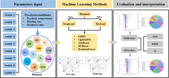
In this paper, previous research literature were collected by entering keywords such as “biochar” and “pyrolysis” in literature search engines, such as Scopus and Google Scholar. To realize the ML model prediction of biomass char yield and SSA, 622 datasets were collected from the literature survey. The datasets were obtained by collecting relevant data from the literature by using the biomass properties and pyrolysis conditions as variables and descriptors, and the SSA and total void volume of biochar as output variables. In the literature, our main focus was on analyzing the proximate and elemental composition of the biomass feedstock. Specifically, the composition was examined in terms of dry basis for volatile matter (VM), ash (Ash), fixed carbon (FC), and the summed percentage of carbon, hydrogen, nitrogen, and oxygen (C-H-N-O) that adds up to 100. Additionally, the pyrolysis conditions of biochar, including pyrolysis temperature (T), retention time (RT), and pyrolysis rate (HR), were investigated. When collecting data, nonuniformity was encountered in the units used. To address this, the units for the 10 characteristic parameters were standardized as follows: VM, Ash, FC, and C-H-N-O are expressed as mass shares (%), while T, RT, and HR are measured in degrees Celsius (°C), minutes (min), and degrees Celsius per minute (°C/min), respectively. For the dataset used, the content of S in the biomass was not considered an input for the ML prediction because the content of S compared with the other elements was very low (negligible) or not provided in the collected data. Proximate analyses were harmonized based on a dry basis, whereas elemental compositions were harmonized based on ashless and dry bases, and O was calculated from the difference.
O = 100 − C-H-N-S (if available),
Ash + FC + VM = 100
2.2. Dataset Preprocessing
In the dataset, the feature data with less than 70% of feature collection were removed and find and data removal. For missing values in the collected data, five ways of filling missing values (polynomial filling, 0-value filling, median filling, mean filling, and linear filling) were conducted, and linear filling by empirical comparison was used [25]. The literature was searched for 622 data on biochar, including biomass feedstocks such as macroalgae, rice husk, corn stover bark, sewage sludge, bamboo chips, corn stover, bagasse, swine manure, pine chips, digestate, soybean oil cake, municipal biosolid waste, yak manure, walnut shells, rice straw, coconut shells, palm kernel shells, and food waste digestate, and four major items were collected, namely, elemental composition (C, H, O, and N content), proximate composition (ash, FC, and volatiles), and pyrolysis conditions (pyrolysis temperature, heating rate, and RT), where the SSA and yield of biochar were also collected. Table 1 shows the specific distribution of each characteristic in the dataset:
In this paper, the linear correlation between any two continuous variables and between the input and target variables is represented by the Pearson correlation coefficient (PCC) [26], which is given by the following Formula (3):
where and denote the mean values of x and y (input and target variables), respectively. In addition, the PCC obeys a t distribution with degrees of freedom (n − 2), and the significance level test [27] can be found by the following Equation (4):
2.3. Standardization of Datasets
In the provided sample data, different evaluation indicators (i.e., features in the eigenvectors) commonly have varying scales and units of measurement. This discrepancy can affect the results of data analysis. To mitigate the influence of these scale differences, the sample data need to be standardized. The goal is to address variations and enable comparability between the different data indicators. Normalization is carried out to ensure that the data for each indicator are brought to the same order of magnitude. The purpose of normalization is to confine the preprocessed data within a specific range of values, such as [0,1] or [−1, 1]. This approach helps mitigate any detrimental effect caused by outliers or extreme values in the sample data. In summary, normalization is performed to achieve a standardized range for the preprocessed data, ensuring they are comparable and eliminating any negative effect caused by individual data points.
The dataset contains 10 features with different units, requiring preprocessing for standardization and normalization to convert dissimilar data norms to the same specification [28]. Z-score normalization is based on the fact that after the data () is centered by the mean () and then scaled by the standard deviation (), the data obey a normal distribution with a mean of 0 and variance of 1 (i.e., the standard normal distribution), and from this, the normalized value of x and can then be obtained using the following Formula (5):
The individual preprocessed datasets undergo multiple training iterations using randomly selected subsets for training and testing. In this process, 70% of the total data points are randomly assigned as the training set, while the remaining 30% is used as the testset to assess the performance of the developed model. During the training process of the data, we used grid search to tune the hyperparameters During the training process, grid search (GridSearchCV) was used to tune the hyperparameters, where the number of cross-validations was five (cv = 5) to improve the prediction and generalisation ability of the model [29].
In k-fold cross-validation, the training dataset is divided into k subsets of equal size. During each iteration of the training, one subset is used as the validation set, while the k−1 remaining subsets are used as the training set. This approach ensures each subset is used as validation and training data [30]. For each subset, the model is trained using the training set and evaluated using the validation set. This process is repeated k times, with each subset serving as the validation set once. The performance of the model is measured by recording the accuracy or other evaluation metrics obtained from each iteration. By averaging the results from the k iterations, a more reliable estimate of the model’s performance is obtained. This approach facilitates the efficient use of all available data for training and evaluation and avoids the potential issue of having insufficient data for separate training and testsets, enabling a more accurate assessment of the model’s performance.
2.4. Machine Learning Models
Integration learning [31] is a very popular ML algorithm nowadays, our goal is to learn a model that is stable and performs better in all aspects, and the integration learning model combines multiple weak learners to obtain a more comprehensive strong learner to derive the modeling results, with very good strategies on various sizes of datasets. The main ideas of integrated learning are Bagging, Boosting, and Stacking. Boosting and Bagging use the same kind of base learner, so they are generally called homogeneous integration methods. Stacking is usually based on the integration of multiple different base learners, so it is called heterogeneous integration method. This paper focuses on homogeneous integration algorithms, and the RandomForest used here belongs to the Bagging idea, whereas Adaboost, XGBoost, GBDT and LightGBM belong to the Boosting idea.
2.4.1. RandomForest
RandomForest is a Bagging-based integrated learning model algorithm used to make predictions by building multiple decision tree models [32]. RandomForest is one of the widely used algorithms in the field nowadays, and its basic idea is to train each decision tree randomly with put back in the sample data set to ensure each decision tree has a certain degree of variability. Within the decision tree, the nodes are divided by randomly selecting features themselves as candidate dividing features, thus reducing correlation [33]. The Random Forest regression algorithm can improve the stability and generalization of the model by integrating the prediction results from multiple decision trees [34]. Moreover, the risk of overfitting the model can be reduced by random sampling and random feature selection. This approach improves the performance and flexibility of the RandomForest regression algorithm in handling regression problems.
2.4.2. Adaboost
The Adaboost algorithm is an integrated learning method that utilizes Boosting. Its basic concept is to obtain the final regression result by weighted averaging the predictions of multiple weak regression models [35]. Each weak model tries to fit the residuals between the target variable and the current model prediction in each iteration. The search mechanism used by the typical Adaboost algorithm is the backtracking method, which does not ensure the selected weighted ones are the overall best, although a greedy algorithm is used to obtain the locally best weak classifiers at each iteration during the training of the weak classifiers. After selecting the weak classifier with the smallest error, the weights of each sample are updated to increase the weights corresponding to the misclassified samples and relatively decrease the weights of the correctly classified samples.
2.4.3. XGBoost
XGBoost is a more advanced, flexible, and complex Boosting algorithm compared with Adaboost [36]. In the XGBoost algorithm, the weights of the weak learner are trained by optimizing the anytime function by using the gradient and the second-order derivatives to adjust the weights of the model [37]. The customized loss function used in the algorithm is optimized by means of gradient boosting in each round of get band [38]. Moreover, XGBoost introduces regularization strategies and feature selection techniques to improve the generalization ability of the model and prevent overfitting. The base learners supported by XGBoost include decision trees and linear models, and only the case of only common trees is discussed [39]. Based on the tree-based base learner, XGBoost sets its complexity as the regularization term (6):
In the given equation, T represents the number of leaf nodes in the tree f. Vector is formed by the output values of all the leaf nodes. corresponds to the square of the L2 norm (or modulus) of this vector. Additionally, the equation includes hyperparameters and .
2.4.4. GBDT
GBDT is a type of integrated learning method, which is an algorithm that makes predictions by combining multiple decision trees. Gradient Boosting is an iterative algorithm. Each round fits a new decision tree on the residuals of the previous round. By continuously reducing the model to the residuals of you and error, a strong prediction model is finally obtained [34]. The GBDT algorithm differs from other integrated algorithms in that it uses the idea of Gradient Boosting for modeling, and each decision tree reduces the bias of the model by fitting the residuals of the prediction of the previous round. In the training of each decision tree (weak classifier), GBDT considers feature selection. GBDT determines the importance of features by calculating their gradients and residuals to decide whether the node should be split. Because the training of GBDT is sequential iteration, it is less tolerant to noise and outliers; therefore, it is less robust.
2.4.5. LightGBM
Microsoft developed LightGBM, a framework based on the GBDT algorithm. It is an efficient, distributed gradient boosting framework for solving classification and regression problems [37]. Compared with Adaboost, XGBoost, and GBDT, it uses histogram-based algorithms and sparse feature inference, which makes it highly fast and efficient in training and prediction; it also supports the processing of sparse data and can deal with a large number of features containing zero values. In conclusion, LightGBM is a powerful, efficient gradient boosting framework for large-scale datasets and ML tasks that require high accuracy [39]. Its fast, low memory footprint and customizable features make it widely used and recognized in practical applications.
2.5. Metrics for Machine Learning Model Evaluation
In this paper, five different ML algorithms were used for the SSA and yield of biochar, and the biochar data were analyzed in Python. The datasets were randomly assigned as training and testsets at the ratio of 7:3, and all ML regression models were tuned with hyperparameters using the grid search method and cv = 5 (the number of cross-validations). In this study, we evaluate and compare all machine learning algorithms based on their degree of fit and effectiveness in five integrated models: mean square error (MSE) (7), root mean square error (RMSE) (8), and correlation coefficient (R2) (9). In different models, each piece of data in the dataset has an actual value and a predicted value . The formulas for the three evaluation model metrics (m denotes the size of the dataset) used are as follows:
In the above three formulas, m denotes the size of the dataset, and denotes the average of the predicted values.
2.6. Feature Importance Analysis for Machine Learning Models
Prediction is machine learning’s strong suit, while model interpretation is its shortcoming. Therefore, the article’s explanation through data analysis is divided into two main parts: the ordering of importance of data features, and the relationship between independent and dependent variables.
SHAP (SHapley Additive exPlanation) is a Python “model interpretation” package that can interpret the output of any machine learning model. Inspired by cooperative game theory, SHAP builds an additive explanatory model where all features are considered “contributors” [40]. For each prediction sample, the model produces a prediction value, and the SHAP value is the value assigned to each feature in the sample. This interpreter integrates ML models to study the correlation between inputs and outputs. Using the SHAP values calculated based on game theory, the ML integrated interpreter is utilized to determine the importance of each feature to the target [41]. The SHAP approach grants a value for each data point of the input feature to reflect its local importance on the target feature. It plays a vital role in enhancing model interpretability, explainability, and credibility and helps better understand and trust the decision making of ML models.
Hence, scatter plots and pie charts depicting feature importance are generate by ranking the significant features in the model according to their SHAP values. This is achieved utilizing built-in functions from the SHAP library in Python.
3. Results
3.1. Statistical Analysis of Sample Data
The violin diagram is a commonly used data visualization tool to show the distribution of data and probability density estimation. The width of the violin plot can reflect the distribution density of the data; the wider the width, the higher the data density of the data variable, and vice versa. Box-and-line plots within the violin plot show the median, quartiles, and outliers of the data, which are statistics that provide the concentration of the data and the degree of dispersion. Figure 1 shows a violin plot of the distribution of features of the collected dataset, and all the features are concentrated around the median. Table 1 lists the 12 features considered in this work, their names, median, mean, standard deviation, and quartiles. In Figure 1, the elemental composition of the biochar (i.e., C, H, O, and N), C and O are high, with C predominantly between 33% and 62% and O distributed around 25% to 57%. The level of O content has a substantial effect on the pore structure and chemical reactivity of the biochar, and biochar with a high oxygen content may result in a lower SSA and smaller pore volume, which may affect its adsorption capacity, storage capacity, and mass transfer properties; biochar with high oxygen content may exhibit higher reactivity in certain chemical reactions. This outcome may influence the effectiveness of biochar for environmental applications, soil amendment, or as an adsorbent. For the proximate composition of biochar (volatiles, ash, and FC), the volatiles are concentrated between 65% and 89% and the ash content is generally low, which correlates with the raw material, pyrolysis conditions, and the way the biochar was prepared. For the pyrolysis conditions (heating temperature, heating rate, and residence time), all three span a wide range because of the stochastic nature.
The correlation between features cannot yet be described more clearly through violin plots, and the PCC measures the degree of linear correlation between two continuous variables. Figure 2 shows the correlation coefficient has a range of values between −1 and 1. When p (correlation coefficient) is close to 1, a strong positive correlation exists between the two variables, that is, when one variable increases, the other increases. When p is close to −1, a strong negative correlation exists between the two variables, that is, when one variable increases, the other decreases. In the graph, ash content (p = 0.378) and N yield (p = 0.283) are positively correlated, which indicates an increase in ash content and N yield increases biochar production [41,42,43]. Except for temperature (p = −0.519), which has a negative correlation, the other characteristics have a slight effect on biochar yield. The SSA of biochar is one of its key characteristics, the size of the SSA value directly affects its functional utility, and the adsorption performance, chemical reaction activity, and pore structure of biochar are all directly related to the SSA characteristic. The figure shows the SSA of biochar has a positive correlation with temperature (p = 0.351), FC content (p = 0.302), and heating rate (p = 0.275). Appropriate temperatures can promote the carbonization, volatile molecule release, and pore structure formation of biochar, thus increasing the SSA. However, an extremely high temperature may lead to sintering and pore collapse, decreasing the SSA. Therefore, selecting the appropriate temperature during biochar preparation is critical to balance the relationship between pore structure development and char stability to obtain the desired SSA.
3.2. Model Prediction
For model predictions, this paper starts from the two goals out of the biochar yield and the SSA of the biochar, for the five integrated ML models selected for prediction at the same time, their model evaluation indices are recorded, and the ML model that best suits the desired goal is screened.
3.2.1. Machine Learning Models Predicting Comparative Yield Productions
Table 2 dispalays five models: GBDT, LightGBM, Adaboost, XGBoost and RandomForest. These models are used to predict yield and collect data to calculate MSE (mean square error), RMSE (root mean square error), and R2 (correlation coefficient) for both the training and testing datasets. Figure 3 shows the test scatterplot of running the above five integrated ML models, all of which are ML model evaluation metrics derived from the data after five cross-validations. Based on the results of previous work on thermal solution modeling using RandomForest and Artificial Neural Networks, the data after cross-validation can still be considered to have a high degree of precision and accuracy [16,17,18]. Table 2 reveals that on the training dataset, the correlation coefficients of GBDT, LightGBM, and XGBoost are all 0.99, which all have high fit; on the testset, the best performance is from the XGBoost model with an R2 of 0.79.
Figure 3 demonstrates the prediction scatter plots of the five models, namely, GBDT, LightGBM, AdaBoost, XGBoost, and RandomForest. Overall, MSEs of the testset are all larger than those of the training set. This is due to the fact that the errors in the training set are smaller than those in the testset.
Moreover, the five scatter plots reveal the XGBoost model in Figure 4 has a more concentrated scatter among the five algorithms. The model fits the data better, most of the data points are close to the linear regression line predicted by the model, and the data points scatter. A large deviation from the predicted line may be due to other factors or anomalies, and further processing and adjusting these anomalies only may be necessary. The XGBoost model prediction in the feature importance histogram is shown in the annex.
3.2.2. Machine Learning Predicting Comparative Surface Area
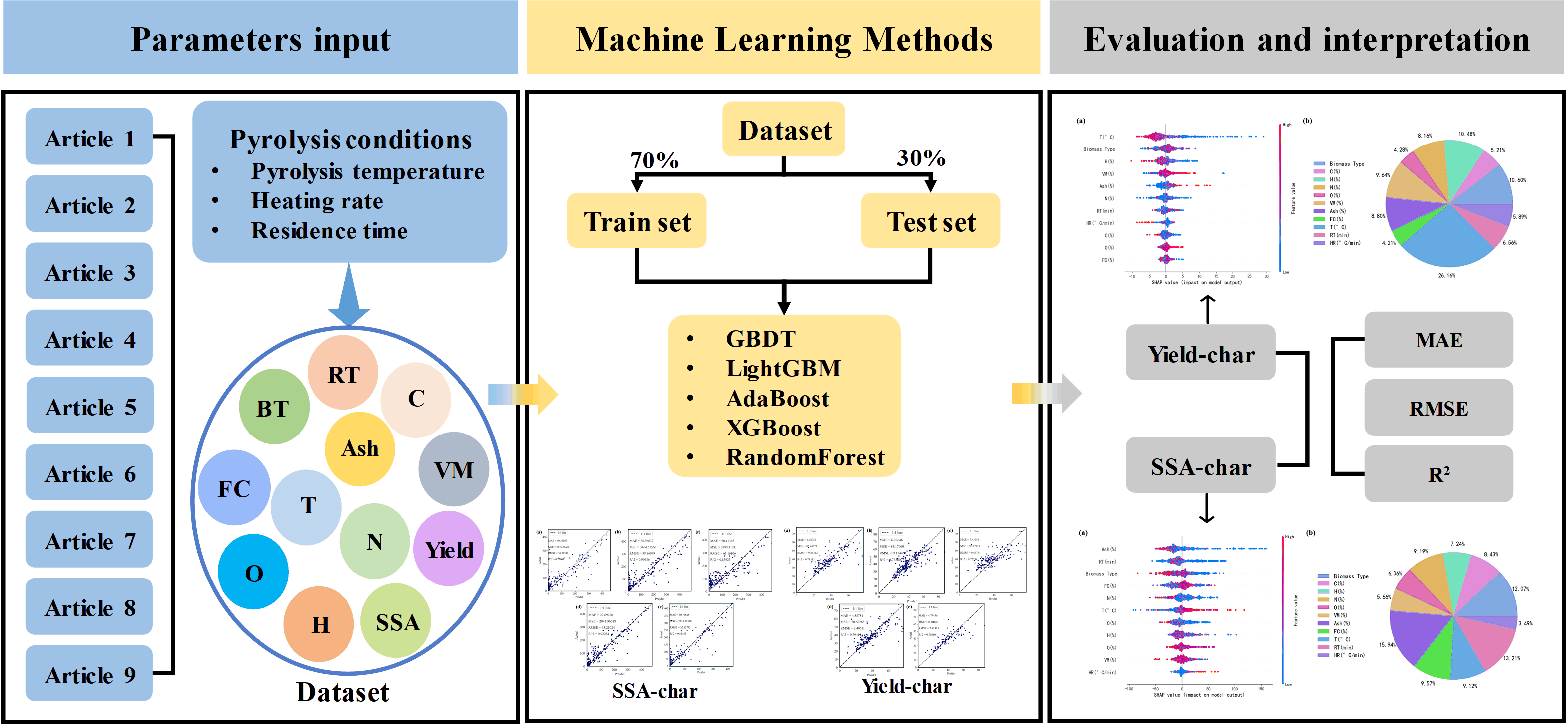
Table 3 counts the MSE, RMSE, and R2 of the training and testing datasets for the five models, namely, GBDT, LightGBM, AdaBoost, XGBoost, and RandomForest, when comparing the surface area to make predictions. Similarly, all five models are ML model evaluation metrics derived from five cross-validations of the data. The R2 for the training set of all five ML models is greater than 0.95, and the XGBoost model has the highest value of 0.92 in the predicted R2 of the testset, which has the best fit among the five models. This situation is mainly because the algorithm itself has measures to prevent overfitting and improve the generalization ability of the model.
Figure 4 demonstrates the predicted scatter plots of the five models, namely, GBDT, LightGBM, AdaBoost, XGBoost, and RandomForest. The horizontal coordinate is the predicted value, and the vertical coordinate is the actual value. The five plots present the relationship between the predicted and actual values of the regression models for the specific surface of biochar. Overall, the regression predictions made by the five algorithms show a linear trend to varying degrees, with XGBoost having the highest R2 of 0.92. To improve the capabilities further, controlling the hyperparameters of XGBoost by customizing the options to tailor the model to the specific problem can also be continued.
3.3. Machine Learning Models Explained
The model’s characteristic importance plots can depict the input parameters with the greatest effect on each of biochar yield and SSA but cannot illustrate how the input parameters affect the target variables. Therefore, this paper uses SHAP dependency plots to illustrate how the input parameters interact with the biochar yield and SSA. SHAP provides a game-theoretic framework for disentangling the degree to which each feature contributes to the model’s predictions.
3.3.1. Explanation of the Yield Prediction Model for Biochar
Figure 5 is a plot of the feature importance analysis of all input parameter features on biochar yield, (a) a feature density scatter plot, which can be seen as a ranked plot of feature importance, and (b) a pie chart of feature share, which demonstrates the share of each feature in the overall dataset. Each row of the feature density scatterplot represents a feature input variable with the horizontal coordinate as the average absolute value of SHAP. A large number of points are in each row, one point represents a sample data, and the color represents the influence on the feature on the SHAP value; the redder the color indicates the larger value, and the bluer indicates the smaller value of the feature.
In Figure 5a, each row is sorted according to the SHAP value of the characteristic input parameters, the temperature was found to be the most influential factor, as indicated by the majority of sample sizes exhibiting significant levels of red pigmentation and a strong negative impact. The current research is also generally performed through the adjustment of the temperature, to control the biochar yield and carbonization degree and quality, and to satisfy the different conditions in the industrial demand. This point of view is consistent with our paper. Moreover, higher temperatures have a larger amount of data and zero effect on the ash, VM, and FC of biochar. The red part of the SHAP value is greater than the 0 bias, which indicates high temperatures have a negative effect on all three of the biochar, indicating ash, VM, and FC do not have much effect on the yield of biochar [16,44,45]. Low temperatures have a positive effect on the yield of biochar. Moreover, the pyrolysis rate affects the production of biochar yield, while the elemental H content also has a negative effect, which suggests the biomass feedstock on high H content has a positive effect on the biochar yield.
The pie chart in Figure 5b shows the highest percentage of pyrolysis temperature (26.16%), followed by biomass feedstock (10.60%), and H content (10.48%) for all the characteristics, which also indicates the main factors affecting biochar yield are these three predominantly. In conclusion, higher pyrolysis temperatures are not favorable to the improvement of biochar yield and are related to the biomass feedstock because high temperatures increase the production of ash, volatiles, and FC.
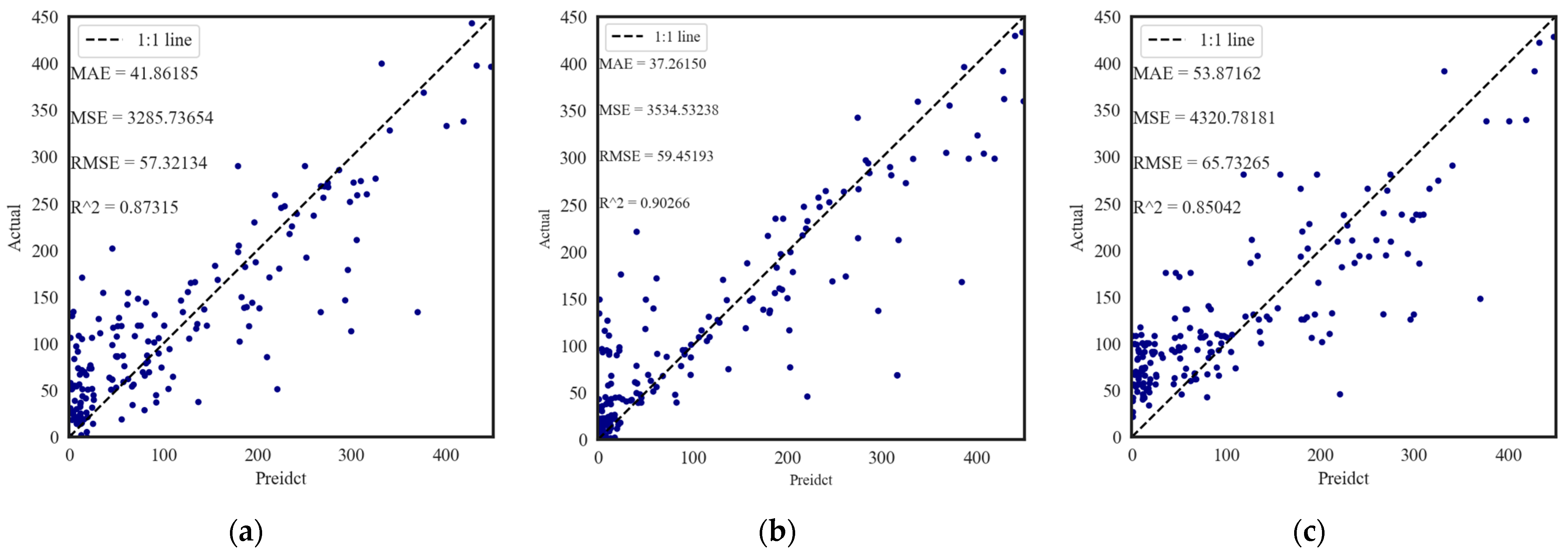
In this paper, the interaction between pyrolysis temperature and other input characterization parameters is analyzed using SHAP dependency plots, as shown in Figure 6a–k. The SHAP dependency plot provides insights into the relative importance of the datasets by plotting the points of each dataset along the x axis, representing the range of the input parameters, and the SHAP values along the y axis, representing the effect on the datasets. The secondary y axis represents the pyrolysis temperature, enabling the identification of the combined effect of pyrolysis temperature and other input parameters. The SHAP plot is a widely used scatter plot based on game theory, which helps explain the influence of individual features on model predictions. Because pyrolysis temperature has the most significant effect on biochar yield, its interaction with other parameters is specifically examined. The magnitude of the SHAP value indicates the strength of its effect on biochar yield. Positive SHAP values suggest a positive contribution to the biochar yield, whereas negative values indicate a reverse effect on the product results. SHAP dependency plots for sparse data points may lack precision and should be disregarded. Therefore, meaningful inferences for all input parameters cannot be obtained solely from SHAP dependency plots. Figure 6k demonstrates the gradual decrease in biochar yield with increasing age pyrolysis temperature. Figure 6b,e,h,i show the dependence scatter plots of the relationship between biochar H, N, C, and O and pyrolysis temperature, where the pyrolysis temperature shows a negative correlation with the H elemental content because the pyrolysis of biochar is accelerated at higher temperatures, which leads to an increase in the rate at which decomposition of the organic matter (including hydrogen-containing compounds) occurs and is converted into gaseous products; no significant linear or nonlinear relationship is observed with the N content. For C and O content, the higher the temperature is, the more completely the carbonization is reflected, and the more C and O content are obtained. Figure 6c,d,j present the subproducts during the pyrolysis of biochar, in agreement with the analysis of Figure 5a, which shows temperature has a negative correlation to varying degrees for ash and FC and a positive correlation for volatiles.
3.3.2. Explanation of the Surface areas Model for Biochar
Figure 7 is a graph of the feature importance analysis of all input parameter features on the SSA of biochar, (a) is a scatter plot of feature density, which can be seen as a ranking of feature importance, and (b) is a pie chart of feature percentage, which shows the percentage of each feature in the overall data set. The feature input parameters with the greatest influence on the SSA of biochar are ash, pyrolysis rate, biomass feedstock, and FC content. In the existing studies, ash is mainly composed of minerals, such as metal oxides and inorganic salts, which are inorganic substances that do not decompose with the pyrolysis reaction but remain in the biochar. Ash contributes to reducing the specific surface area of biochar by blocking voids and covering its surface. In Figure 7a, most of the red dots in the row of ash are densely distributed to the left of the 0 axis, which has a negative correlation effect on the SSA of the biochar, which is in line with many studies. Different biomass feedstocks have diverse organizational structures, moisture contents, fiber structures, and particle sizes as well as different suitable pyrolysis conditions. In Figure 5a, the distribution of the red portion of the biomass feedstock is more dispersed, and the enriched portion is near the right side of the 0 axis, which can indicate the importance of the effect of the raw material of biochar on the SSA. Figure 7b shows the pie chart of the importance of all input features, which corresponds to Figure 7a.
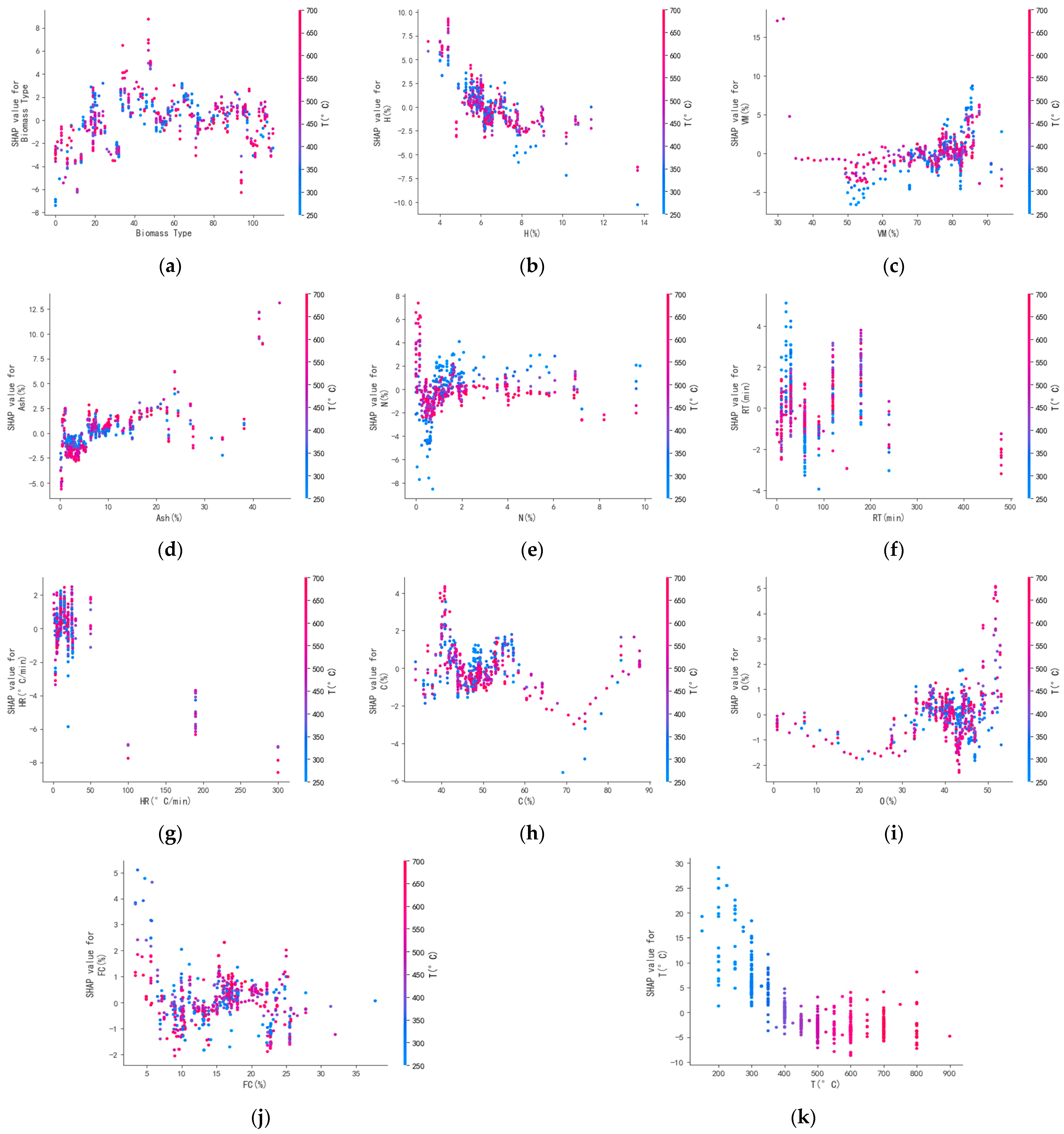
Figure 8a–k show the interaction SHAP dependency plot of ash content with other input feature parameters considered in this paper. Ash, as the first place of feature importance, is represented by the sub y axis, which helps identify the combined effect of ash and other input parameters. Ash has no significant linear relationship with RT, biomass feedstock, and FC content in Figure 8a–c. The distribution of biomass feedstock is dispersed because different materials have dissimilar elemental content, fiber structure, and moisture content and do not show a linear relationship. Similarly, in Figure 8c, the FC content in general shows a negative correlation with the ash content, which is probably because the moisture content, calorific value, and other parties are not considered. Figure 8d shows the higher the SHAP value of the will be divided into instead of the N element content is smaller; this relationship has been a common phenomenon in many studies. Figure 8e shows the relationship between pyrolysis temperature and ash content; the higher the pyrolysis temperature is, the higher the ash content, and the pyrolysis temperature accelerates the completion of the thermal onset conditions; thus, this phenomenon follows the generalized studies. The characteristic input terms in Figure 8f–j do not show a linear relationship with ash exhibited in the graph. Figure 8k shows the SSA decreases with increasing ash content because ash consists mainly of inorganic substances such as minerals and inorganic salts, which are not characterized by high SSA. When the inorganic matter in biochar increases, it occupies more space and reduces the available surface area of the carbonaceous material.
3.4. Compare with Previous Work
Table 4 shows that for the prediction of biochar yield the correlation coefficient (R2) is small in comparison to other studies, however the data set we have collected is larger than the data collected in the above literature; for the prediction of specific surface area it can be seen that our predictions have a small increase in correlation coefficient (R2) in comparison. The above-mentioned studies have shown that the size of the data set can have an impact on our predictions to a certain extent when machine learning is used for the prediction. In comparison with other integrated learning algorithms, it can be seen that XGBoost is a powerful algorithmic tool in its own right with very strong performance and is more suitable for the study of such problems. Based on this, according to our study, we have the following conclusions: the data set can have an impact on the final prediction results; XGBoost outperforms other algorithms in the integrated learning methods.
4. Discussion
In this article, the XGBoost algorithm has the most excellent prediction performance, both in terms of biochar yield and specific surface area. The results in this paper are compared with the previous results and the performance of XGBoost algorithm is excellent for different scenarios, such as predicting the adsorption of gases based on molecular structure and molecular specificity parameter, which also reflects the versatile applicability of XGBoost algorithm. Of course, the XGBoost algorithm used in this article has limitations. For example, the data remembers that the size of the algorithm has a huge impact on the algorithm’s prediction performance, and at the same time in the use of scenarios harmed by the Tao of incomplete data features, so that experiments can be carried out using a variety of features in different combinations. A comprehensive database of biochar-related data is needed to allow researchers to conduct in-depth studies using the current information available. This database should include data on the properties and uses of biochar.
In biochar-related research, the application of machine learning algorithms is an efficient way to enhance research capabilities. High-performance algorithms, such as support vector machines, neural networks, and others, can be utilized in various datasets and problem domains, providing valuable insights and discoveries for the development of biochar research. These algorithms can uncover new patterns and relationships, leading to a deeper understanding of biochar properties.
5. Conclusions
In this paper, the biochar yield with SSA was predicted based on five integrated ML algorithm models, namely, GBDT, LightGBM, AdaBoost, XGBoost, and RandomForest, by utilizing inputs of pyrolysis conditions, elemental composition, and final approximation of analytical data features. The hyperparameter tuning of each model was carried out using grid search, and the R2 of the training and testsets for predicting biochar yield using the XGBoost model were 0.99 and 0.79, respectively, with a large percentage of feature importance of pyrolysis temperature, biomass feedstock, and H content among the input features; the R2 of the training and testsets for predicting the SSA of biochar were 0.96 and 0.92, respectively, with the input features of Ash, biomass feedstock, and H content have a large proportion of feature importance. Examining the importance and SHAP dependency plots discovered notable interactions between the input features and biochar yield. Furthermore, as the amount of data used in the model increased, the model’s robustness improved. To expand on the current study, delving deeper into qualitative aspects such as proximate analysis and the composition of biochar would be beneficial. These factors could provide valuable insights into the optimization of biochar preparation.
There are still some deficiencies in this paper: more complex machine learning algorithms such as neural networks are not used to further improve the performance of the model, and no comparison of machine learning performance with different input feature parameters has been made to see if fewer features can predict. Overall, this paper highlights the significance of input feature interactions and suggests further work is required to understand the optimization of biochar preparation fully.
Supplementary Materials
The following supporting information can be downloaded at: https://www.mdpi.com/article/10.3390/c10010010/s1.
Author Contributions
Conceptualization, X.Z., L.S. and X.L.; methodology, X.Z.; software, X.Z.; validation, X.Z., X.J. and L.S.; formal analysis, X.Z., X.L., L.S. and X.J.; investigation, X.Z., Y.L. and F.T.; resources, X.L., F.T., Y.L. and Z.W.; data curation, X.Z.; writing—original draft preparation, X.Z.; writing—review and editing, X.L.; visualization, X.Z.; supervision, Z.W.; project administration, X.Z.; funding acquisition, X.L., F.T., Y.L. and Z.W. All authors have read and agreed to the published version of the manuscript.
Funding
This work was supported by the National Natural Science Foundation of China (No. 22008186, 22268045, 22278325); Key Research and Development Plan of Shaanxi Province (Nos. 2022NY-056, 2022NY-053); Shaanxi University Youth Science and Technology Innovation Team (2022TD071); Xi’an Association of Science and Technology Youth Talent Promotion Program Project (095920221342); Shaanxi Province Qin Chuangyuan “Scientist + Engineer” Team (2022KXJ-137); Shaanxi University Youth Science and Technology Innovation Team (Grant 2022TD071); Xi'an Key Laboratory of Textile and Chemical Additives Performance Assessment Reward and Subsidy Project (2021JH-201-0004).
Data Availability Statement
Data are contained within the article and Supplementary Materials.
Conflicts of Interest
The authors declare no conflict of interest.
References
- Joselin Herbert, G.M.; Unni Krishnan, A. Quantifying environmental performance of biomass energy. Renew. Sustain. Energy Rev. 2016, 59, 292–308. [Google Scholar] [CrossRef]
- Lee, S.H.; Lum, W.C.; Boon, J.G.; Kristak, L.; Antov, P.; Pędzik, M.; Rogoziński, T.; Taghiyari, H.R.; Lubis, M.A.R.; Fatriasari, W.; et al. Particleboard from agricultural biomass and recycled wood waste: A review. J. Mater. Res. Technol. 2022, 20, 4630–4658. [Google Scholar] [CrossRef]
- Zhao, L.; Wang, Z.; Ren, H.Y.; Chen, C.; Nan, J.; Cao, G.L.; Yang, S.S.; Ren, N.Q. Residue cornstalk derived biochar promotes direct bio-hydrogen production from anaerobic fermentation of cornstalk. Bioresour. Technol. 2021, 320, 124338. [Google Scholar] [CrossRef]
- Liang, Y.; Wang, Y.; Ding, N.; Liang, L.; Zhao, S.; Yin, D.; Cheng, Y.; Wang, C.; Wang, L. Preparation and hydrogen storage performance of poplar sawdust biochar with high specific surface area. Ind. Crops Prod. 2023, 200, 116788. [Google Scholar] [CrossRef]
- Nguyen, Q.A.; Smith, W.A.; Wahlen, B.D.; Wendt, L.M. Total and Sustainable Utilization of Biomass Resources: A Perspective. Front. Bioeng. Biotechnol. 2020, 8, 546. [Google Scholar] [CrossRef] [PubMed]
- Chen, D.; Yin, L.; Wang, H.; He, P. Pyrolysis technologies for municipal solid waste: A review. Waste Manag. 2014, 34, 2466–2486. [Google Scholar] [CrossRef] [PubMed]
- Leng, L.; Huang, H.; Li, H.; Li, J.; Zhou, W. Biochar stability assessment methods: A review. Sci. Total Environ. 2019, 647, 210–222. [Google Scholar] [CrossRef] [PubMed]
- Xiang, W.; Zhang, X.; Chen, J.; Zou, W.; He, F.; Hu, X.; Tsang, D.C.W.; Ok, Y.S.; Gao, B. Biochar technology in wastewater treatment: A critical review. Chemosphere 2020, 252, 126539. [Google Scholar] [CrossRef]
- Lee, D.J.; Cheng, Y.L.; Wong, R.J.; Wang, X.D. Adsorption removal of natural organic matters in waters using biochar. Bioresour. Technol. 2018, 260, 413–416. [Google Scholar] [CrossRef]
- Lyu, H.; Tang, J.; Huang, Y.; Gai, L.; Zeng, E.Y.; Liber, K.; Gong, Y. Removal of hexavalent chromium from aqueous solutions by a novel biochar supported nanoscale iron sulfide composite. Chem. Eng. J. 2017, 322, 516–524. [Google Scholar] [CrossRef]
- Azeem, M.; Hassan, T.U.; Tahir, M.I.; Ali, A.; Jeyasundar, P.G.S.A.; Hussain, Q.; Bashir, S.; Mehmood, S.; Zhang, Z. Tea leaves biochar as a carrier of Bacillus cereus improves the soil function and crop productivity. Appl. Soil Ecol. 2021, 157, 103732. [Google Scholar] [CrossRef]
- Bolan, N.; Hoang, S.A.; Beiyuan, J.; Gupta, S.; Hou, D.; Karakoti, A.; Joseph, S.; Jung, S.; Kim, K.-H.; Kirkham, M.B.; et al. Multifunctional applications of biochar beyond carbon storage. Int. Mater. Rev. 2021, 67, 150–200. [Google Scholar] [CrossRef]
- Leng, L.; Xiong, Q.; Yang, L.; Li, H.; Zhou, Y.; Zhang, W.; Jiang, S.; Li, H.; Huang, H. An overview on engineering the surface area and porosity of biochar. Sci Total Environ. 2021, 763, 144204. [Google Scholar] [CrossRef] [PubMed]
- Choi, M.K.; Park, H.C.; Choi, H.S. Comprehensive evaluation of various pyrolysis reaction mechanisms for pyrolysis process simulation. Chem. Eng. Process.-Process. Intensif. 2018, 130, 19–35. [Google Scholar] [CrossRef]
- Diblasi, C. Modeling chemical and physical processes of wood and biomass pyrolysis. Prog. Energy Combust. Sci. 2008, 34, 47–90. [Google Scholar] [CrossRef]
- Zhu, X.; Li, Y.; Wang, X. Machine learning prediction of biochar yield and carbon contents in biochar based on biomass characteristics and pyrolysis conditions. Bioresour. Technol. 2019, 288, 121527. [Google Scholar] [CrossRef] [PubMed]
- Cao, H.; Xin, Y.; Yuan, Q. Prediction of biochar yield from cattle manure pyrolysis via least squares support vector machine intelligent approach. Bioresour. Technol. 2016, 202, 158–164. [Google Scholar] [CrossRef]
- Muhammad Saleem, I.A. Machine Learning Based Prediction of Pyrolytic Conversion for Red Sea Seaweed. In Proceedings of the Budapest 2017 International Conferences LEBCSR-17, ALHSSS-17, BCES-17, AET-17, CBMPS-17 & SACCEE-17, Budapest, Hungary, 6–7 September 2017. [Google Scholar]
- Tripathi, M.; Sahu, J.N.; Ganesan, P. Effect of process parameters on production of biochar from biomass waste through pyrolysis: A review. Renew. Sustain. Energy Rev. 2016, 55, 467–481. [Google Scholar] [CrossRef]
- Paula, A.J.; Ferreira, O.P.; Souza Filho, A.G.; Filho, F.N.; Andrade, C.E.; Faria, A.F. Machine Learning and Natural Language Processing Enable a Data-Oriented Experimental Design Approach for Producing Biochar and Hydrochar from Biomass. Chem. Mater. 2022, 34, 979–990. [Google Scholar] [CrossRef]
- Ganaie, M.A.; Hu, M.; Malik, A.K.; Tanveer, M.; Suganthan, P.N. Ensemble deep learning: A review. Eng. Appl. Artif. Intell. 2022, 115, 105151. [Google Scholar] [CrossRef]
- Yang, Y.; Lv, H.; Chen, N. A Survey on ensemble learning under the era of deep learning. Artif. Intell. Rev. 2022, 56, 5545–5589. [Google Scholar] [CrossRef]
- Srungavarapu, C.S.; Sheik, A.G.; Tejaswini, E.S.S.; Mohammed Yousuf, S.; Ambati, S.R. An integrated machine learning framework for effluent quality prediction in Sewage Treatment Units. Urban Water J. 2023, 20, 487–497. [Google Scholar] [CrossRef]
- Tsai, W.; Wang, S.; Chang, C.; Chien, S.; Sun, H. Cleaner production of carbon adsorbents by utilizing agricultural waste corn cob. Resour. Conserv. Recycl. 2001, 32, 43–53. [Google Scholar] [CrossRef]
- Emmanuel, T.; Maupong, T.; Mpoeleng, D.; Semong, T.; Mphago, B.; Tabona, O. A survey on missing data in machine learning. J. Big Data 2021, 8, 140. [Google Scholar] [CrossRef]
- Were, K.; Bui, D.T.; Dick, Ø.B.; Singh, B.R. A comparative assessment of support vector regression, artificial neural networks, and random forests for predicting and mapping soil organic carbon stocks across an Afromontane landscape. Ecol. Indic. 2015, 52, 394–403. [Google Scholar] [CrossRef]
- Sun, Y.; Zheng, W.; Zhang, L.; Zhao, H.; Li, X.; Zhang, C.; Ma, W.; Tian, D.; Yu, K.H.; Xiao, S.; et al. Quantifying the Impacts of Pre- and Post-Conception TSH Levels on Birth Outcomes: An Examination of Different Machine Learning Models. Front. Endocrinol. 2021, 12, 755364. [Google Scholar] [CrossRef]
- Zhu, X.; Wan, Z.; Tsang, D.C.W.; He, M.; Hou, D.; Su, Z.; Shang, J. Machine learning for the selection of carbon-based materials for tetracycline and sulfamethoxazole adsorption. Chem. Eng. J. 2021, 406, 126782. [Google Scholar] [CrossRef]
- Morales-Hernández, A.; Van Nieuwenhuyse, I.; Rojas Gonzalez, S. A survey on multi-objective hyperparameter optimization algorithms for machine learning. Artif. Intell. Rev. 2022, 56, 8043–8093. [Google Scholar] [CrossRef]
- Grimm, K.J.; Mazza, G.L.; Davoudzadeh, P. Model Selection in Finite Mixture Models: A k-Fold Cross-Validation Approach. Struct. Equ. Model. A Multidiscip. J. 2016, 24, 246–256. [Google Scholar] [CrossRef]
- Hoarau, A.; Martin, A.; Dubois, J.-C.; Le Gall, Y. Evidential Random Forests. Expert Syst. Appl. 2023, 230, 120652. [Google Scholar] [CrossRef]
- Tirink, C.; Piwczynski, D.; Kolenda, M.; Onder, H. Estimation of Body Weight Based on Biometric Measurements by Using Random Forest Regression, Support Vector Regression and CART Algorithms. Animal 2023, 13, 798. [Google Scholar] [CrossRef]
- Zhao, T.; Liu, S.; Xu, J.; He, H.; Wang, D.; Horton, R.; Liu, G. Comparative analysis of seven machine learning algorithms and five empirical models to estimate soil thermal conductivity. Agric. For. Meteorol. 2022, 323, 109080. [Google Scholar] [CrossRef]
- Barrow, D.K.; Crone, S.F. A comparison of AdaBoost algorithms for time series forecast combination. Int. J. Forecast. 2016, 32, 1103–1119. [Google Scholar] [CrossRef]
- Dong, J.; Chen, Y.; Yao, B.; Zhang, X.; Zeng, N. A neural network boosting regression model based on XGBoost. Appl. Soft Comput. 2022, 125, 109067. [Google Scholar] [CrossRef]
- Tasneem, S.; Ageeli, A.A.; Alamier, W.M.; Hasan, N.; Safaei, M.R. Organic catalysts for hydrogen production from noodle wastewater: Machine learning and deep learning-based analysis. Int. J. Hydrogen Energy 2023, 52, 599–616. [Google Scholar] [CrossRef]
- Pathy, A.; Meher, S.P.B. Predicting algal biochar yield using eXtreme Gradient Boosting (XGB) algorithm of machine learning methods. Algal Res. 2020, 50, 102006. [Google Scholar] [CrossRef]
- Shehadeh, A.; Alshboul, O.; Al Mamlook, R.E.; Hamedat, O. Machine learning models for predicting the residual value of heavy construction equipment: An evaluation of modified decision tree, LightGBM, and XGBoost regression. Autom. Constr. 2021, 129, 103827. [Google Scholar] [CrossRef]
- Wu, Y.; Zhou, Y. Hybrid machine learning model and Shapley additive explanations for compressive strength of sustainable concrete. Constr. Build. Mater. 2022, 330, 127298. [Google Scholar] [CrossRef]
- Fahmi, R.; Bridgwater, A.V.; Donnison, I.; Yates, N.; Jones, J.M. The effect of lignin and inorganic species in biomass on pyrolysis oil yields, quality and stability. Fuel 2008, 87, 1230–1240. [Google Scholar] [CrossRef]
- Li, W.; Dang, Q.; Brown, R.C.; Laird, D.; Wright, M.M. The impacts of biomass properties on pyrolysis yields, economic and environmental performance of the pyrolysis-bioenergy-biochar platform to carbon negative energy. Bioresour. Technol. 2017, 241, 959–968. [Google Scholar] [CrossRef]
- Xu, S.; Chen, J.; Peng, H.; Leng, S.; Li, H.; Qu, W.; Hu, Y.; Li, H.; Jiang, S.; Zhou, W.; et al. Effect of biomass type and pyrolysis temperature on nitrogen in biochar, and the comparison with hydrochar. Fuel 2021, 291, 120128. [Google Scholar] [CrossRef]
- Angin, D. Effect of pyrolysis temperature and heating rate on biochar obtained from pyrolysis of safflower seed press cake. Bioresour. Technol. 2013, 128, 593–597. [Google Scholar] [CrossRef] [PubMed]
- Bridgwater, A.V. Review of fast pyrolysis of biomass and product upgrading. Biomass Bioenergy 2012, 38, 68–94. [Google Scholar] [CrossRef]
- Alabdrabalnabi, A.; Gautam, R.; Mani Sarathy, S. Machine learning to predict biochar and bio-oil yields from co-pyrolysis of biomass and plastics. Fuel 2022, 328, 125303. [Google Scholar] [CrossRef]
- Li, H.; Ai, Z.; Yang, L.; Zhang, W.; Yang, Z.; Peng, H.; Leng, L. Machine learning assisted predicting and engineering specific surface area and total pore volume of biochar. Bioresour. Technol. 2023, 369, 128417. [Google Scholar] [CrossRef]
- Li, L.; Zhao, Y.; Yu, H.; Wang, Z.; Zhao, Y.; Jiang, M. An XGBoost Algorithm Based on Molecular Structure and Molecular Specificity Parameters for Predicting Gas Adsorption. Langmuir 2023, 39, 6756–6766. [Google Scholar] [CrossRef] [PubMed]
Figure 1.
Distribution of violins in the dataset.

Figure 2.
Heatmap of Pearson correlation analysis of sample data.

Figure 3.
Scatterplot of yield prediction of biochar by five algorithms, GBDT (a), LightGBM (b), AdaBoost (c), XGBoost (d), and RandomForest (e), on the testset.
Figure 3.
Scatterplot of yield prediction of biochar by five algorithms, GBDT (a), LightGBM (b), AdaBoost (c), XGBoost (d), and RandomForest (e), on the testset.

Figure 4.
Scatterplot of specific surface area of biochar by five algorithms, GBDT (a), LightGBM (b), AdaBoost (c), XGBoost (d), and RandomForest (e), on the testset.
Figure 4.
Scatterplot of specific surface area of biochar by five algorithms, GBDT (a), LightGBM (b), AdaBoost (c), XGBoost (d), and RandomForest (e), on the testset.


Figure 5.
Characteristic importance analysis plot affecting biochar yield, (a) scatter plot of characteristic density and (b) pie chart of characteristic importance.
Figure 5.
Characteristic importance analysis plot affecting biochar yield, (a) scatter plot of characteristic density and (b) pie chart of characteristic importance.

Figure 6.
SHAP dependency plot of the joint effect of temperature and other input parameters on biochar yield using XGBoost model. ((a–k) correspond sequentially to data characteristics of biomass feedstock (Biomass Type), H content, Volatile Matter content (VM), Ash content (Ash), N content, Retention Time (RT), Heating Rate (HR), C content, O content, Fixed Carbon content (FC), and Pyrolysis Temperature (T).).

Figure 7.
Characteristic importance analysis plots affecting the specific surface area of biochar, (a) scatter plot of characteristic density and (b) pie chart of characteristic importance.
Figure 7.
Characteristic importance analysis plots affecting the specific surface area of biochar, (a) scatter plot of characteristic density and (b) pie chart of characteristic importance.

Figure 8.
SHAP dependency plot of the joint effect of ash and other input parameters on biochar yield using XGBoost model. ((a–k) correspond sequentially to data characteristics of retention time (RT), biomass feedstock (Biomass Type), fixed carbon content (FC), N content, pyrolysis temperature (T), C content, H content, O content, volatile matter content (VM), heating rate (HR), and ash content (Ash).).


Table 1.
Statistical analysis of all features involved in machine learning models for yield and specific surface area.
Table 1.
Statistical analysis of all features involved in machine learning models for yield and specific surface area.
| C | H | O | N | VM | Ash | FC | T | RT | HR | Yield-Char | SSA-Char | |
|---|---|---|---|---|---|---|---|---|---|---|---|---|
| count | 593 | 593 | 593 | 577 | 521 | 597 | 506 | 622 | 622 | 617 | 474 | 348 |
| mean | 48.44 | 6.41 | 1.92 | 40.93 | 76.33 | 7.75 | 21.55 | 476.22 | 69.23 | 19.95 | 38.97 | 80.15 |
| std | 9.84 | 1.37 | 3.98 | 9.17 | 9.01 | 7.72 | 58.13 | 147.25 | 70.65 | 38.75 | 14.75 | 112.08 |
| min | 4.80 | 3.42 | 0 | 0.87 | 27.62 | 0.16 | 3.37 | 30 | 1 | 1 | 9.17 | 0.02 |
| 25% | 43.92 | 5.81 | 0.49 | 39.37 | 72.95 | 2.42 | 11.25 | 356.25 | 30 | 10 | 28.52 | 4.97 |
| 50% | 47.75 | 6.19 | 1.07 | 42.54 | 77.75 | 6.04 | 16.49 | 500 | 60 | 10 | 35.77 | 25.63 |
| 75% | 51.01 | 6.70 | 1.89 | 45.51 | 82.38 | 9.86 | 20.09 | 600 | 60 | 18 | 47.04 | 98.33 |
| max | 87.62 | 13.67 | 40.41 | 63.34 | 94.16 | 45.54 | 600 | 900 | 480 | 300 | 93.50 | 525.86 |
Table 2.
Statistics of three evaluation metrics of five algorithms GBDT, LightGBM, AdaBoost, XGBoost and RandomForest for predicting biochar production.
Table 2.
Statistics of three evaluation metrics of five algorithms GBDT, LightGBM, AdaBoost, XGBoost and RandomForest for predicting biochar production.
| Yield-Char (%) | ||||||
|---|---|---|---|---|---|---|
| Train Set | Test Set | |||||
| MSE | RMSE | R2 | MSE | RMSE | R2 | |
| GBDT | 23.05 | 4.80 | 0.99 | 85.44 | 9.24 | 0.75 |
| LightGBM | 21.52 | 4.64 | 0.99 | 85.83 | 9.26 | 0.75 |
| AdaBoost | 24.63 | 4.96 | 0.96 | 96.78 | 9.84 | 0.72 |
| XGBoost | 22.51 | 4.75 | 0.99 | 70.66 | 8.41 | 0.79 |
| RandomForest | 15.18 | 3.90 | 0.98 | 61.05 | 7.81 | 0.71 |
Table 3.
Statistics of three evaluation metrics of five algorithms GBDT, LightGBM, AdaBoost, XGBoost and RandomForest for predicting specific surface area.
Table 3.
Statistics of three evaluation metrics of five algorithms GBDT, LightGBM, AdaBoost, XGBoost and RandomForest for predicting specific surface area.
| SSA-Char (%) | ||||||
|---|---|---|---|---|---|---|
| Train Set | Test Set | |||||
| MSE | RMSE | R2 | MSE | RMSE | R2 | |
| GBDT | 1043.77 | 32.31 | 0.98 | 3285.73 | 57.32 | 0.87 |
| LightGBM | 1352.46 | 36.78 | 0.96 | 3534.53 | 59.45 | 0.90 |
| AdaBoost | 1230.90 | 35.08 | 0.97 | 4320.78 | 65.73 | 0.85 |
| XGBoost | 1031.07 | 32.11 | 0.96 | 2043.97 | 45.21 | 0.92 |
| RandomForest | 1071.65 | 31.90 | 0.97 | 2718.36 | 52.14 | 0.81 |
Table 4.
Comparison of model predictions of biochar yield and specific surface area.
| Model Method | Performance Prediction | Data Volume | Model Performance | Ref. |
|---|---|---|---|---|
| XGBoost | Biochar yield | 94 | R2 = 0.96 | [46] |
| Dense neural network | Bio-oil yield | 96 | R2 = 0.96 | |
| XGBoost | Biochar yield | 91 | R2 = 0.75 | [38] |
| Ramdomforest | Biochar yield | 245 | R2 = 0.85 | [16] |
| Ramdomforest | SSA | 169 | R2 = 0.84 | [47] |
| GBR | SSA | 169 | R2 = 0.9 | |
| XGBoost | Biochar yield | 622 | R2 = 0.79 | This study |
| XGBoost | SSA | 622 | R2 = 0.92 |
Disclaimer/Publisher’s Note: The statements, opinions and data contained in all publications are solely those of the individual author(s) and contributor(s) and not of MDPI and/or the editor(s). MDPI and/or the editor(s) disclaim responsibility for any injury to people or property resulting from any ideas, methods, instructions or products referred to in the content. |
© 2024 by the authors. Licensee MDPI, Basel, Switzerland. This article is an open access article distributed under the terms and conditions of the Creative Commons Attribution (CC BY) license (https://creativecommons.org/licenses/by/4.0/).
Share and Cite
MDPI and ACS Style
Zhou, X.; Liu, X.; Sun, L.; Jia, X.; Tian, F.; Liu, Y.; Wu, Z. Prediction of Biochar Yield and Specific Surface Area Based on Integrated Learning Algorithm. C 2024, 10, 10. https://doi.org/10.3390/c10010010
AMA Style
Zhou X, Liu X, Sun L, Jia X, Tian F, Liu Y, Wu Z. Prediction of Biochar Yield and Specific Surface Area Based on Integrated Learning Algorithm. C. 2024; 10(1):10. https://doi.org/10.3390/c10010010
Chicago/Turabian StyleZhou, Xiaohu, Xiaochen Liu, Linlin Sun, Xinyu Jia, Fei Tian, Yueqin Liu, and Zhansheng Wu. 2024. "Prediction of Biochar Yield and Specific Surface Area Based on Integrated Learning Algorithm" C 10, no. 1: 10. https://doi.org/10.3390/c10010010
Note that from the first issue of 2016, this journal uses article numbers instead of page numbers. See further details here.