
On the Magnetization and Entanglement Plateaus in One-Dimensional Confined Molecular Magnets


Abstract
:1. Introduction
2. Trimetric Ni-Based Single Chain Magnets and Quantum Methods
2.1. Spin Chains: Hamiltonian Modeling
2.2. Quantum Many-Body Methods: DMRG and MPS
3. 3D and 1D Molecular Magnets
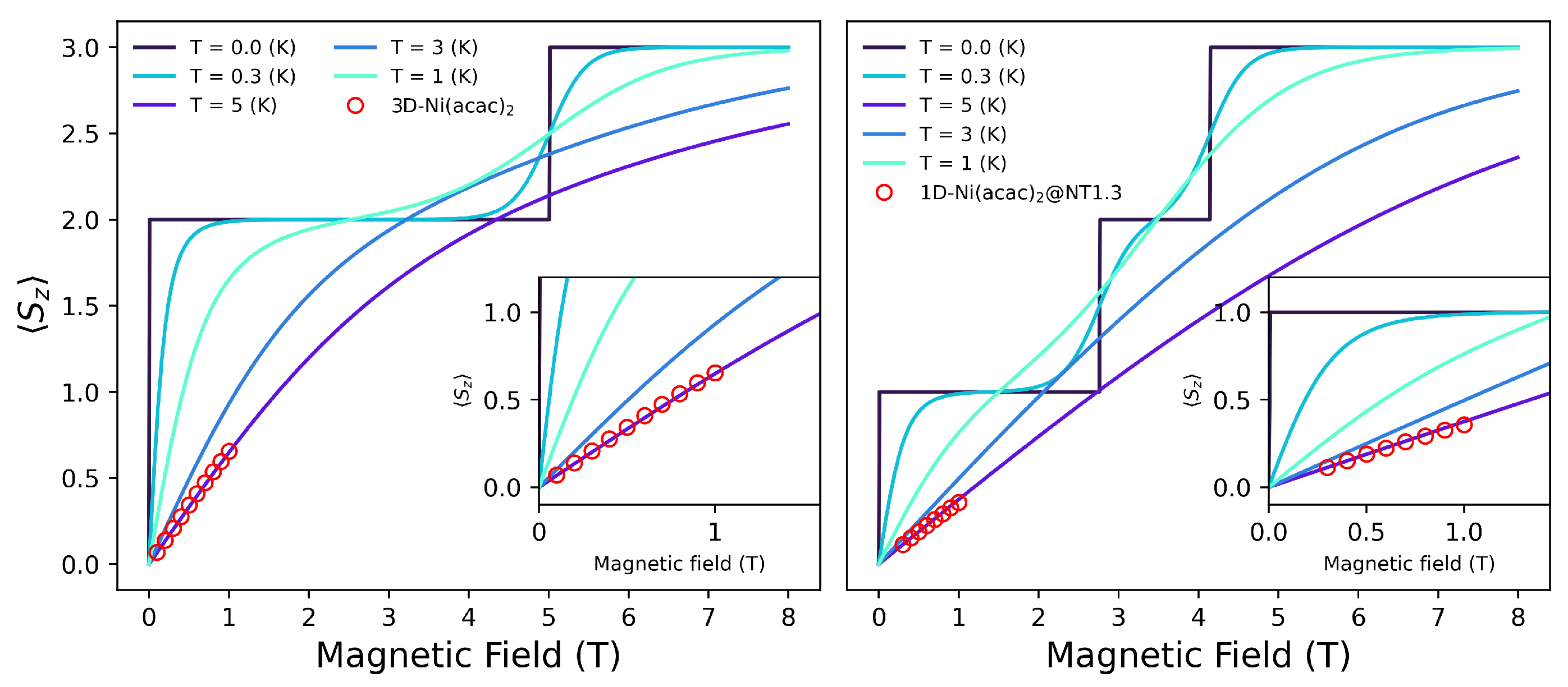
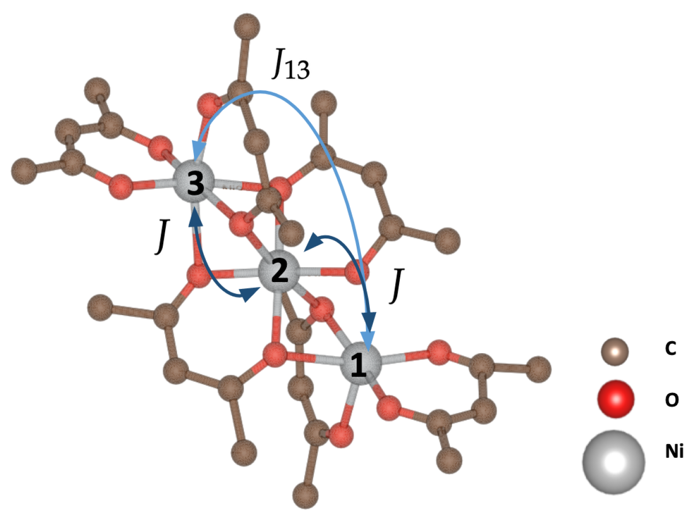
3.1. SMM Solutions
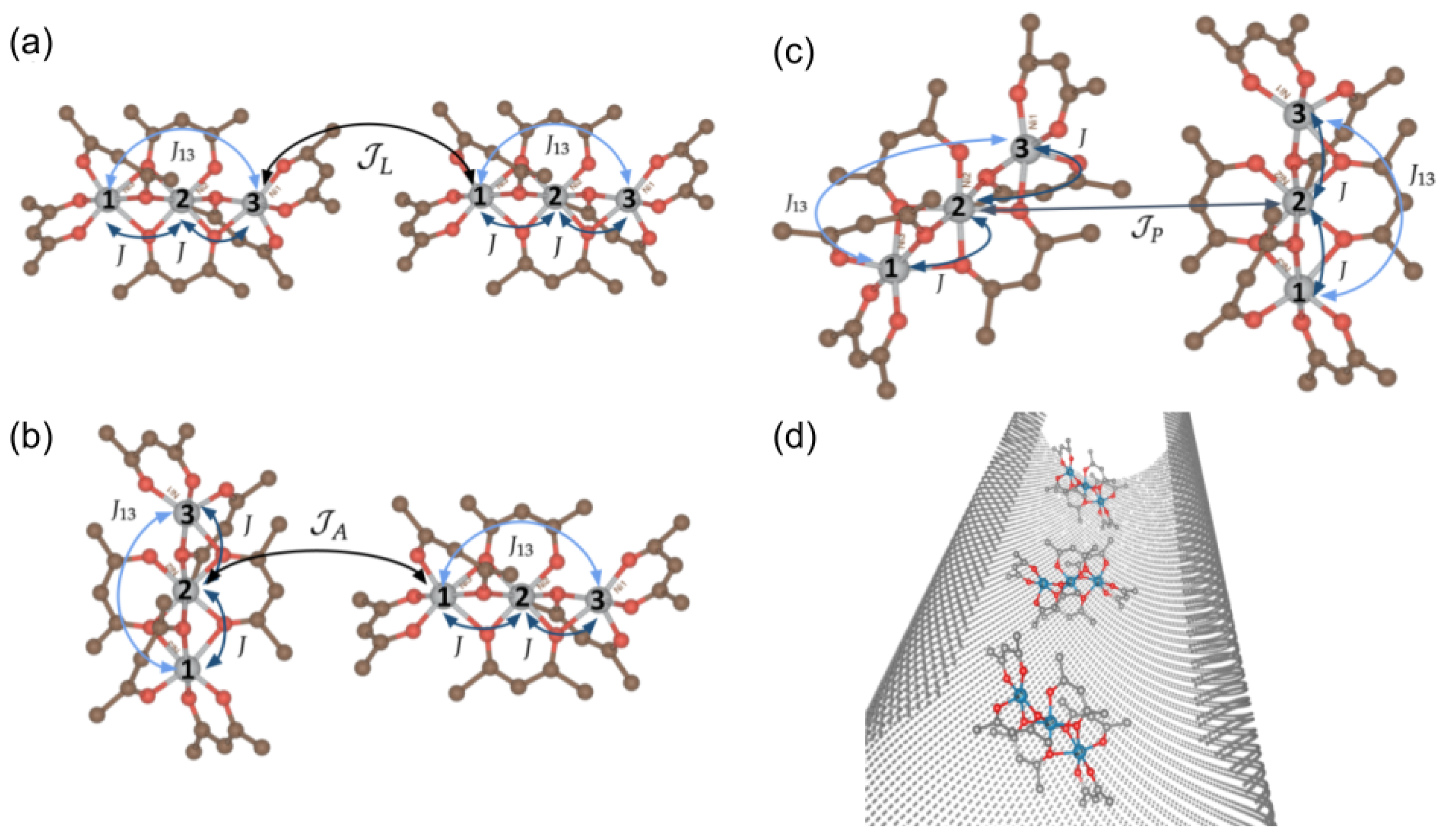
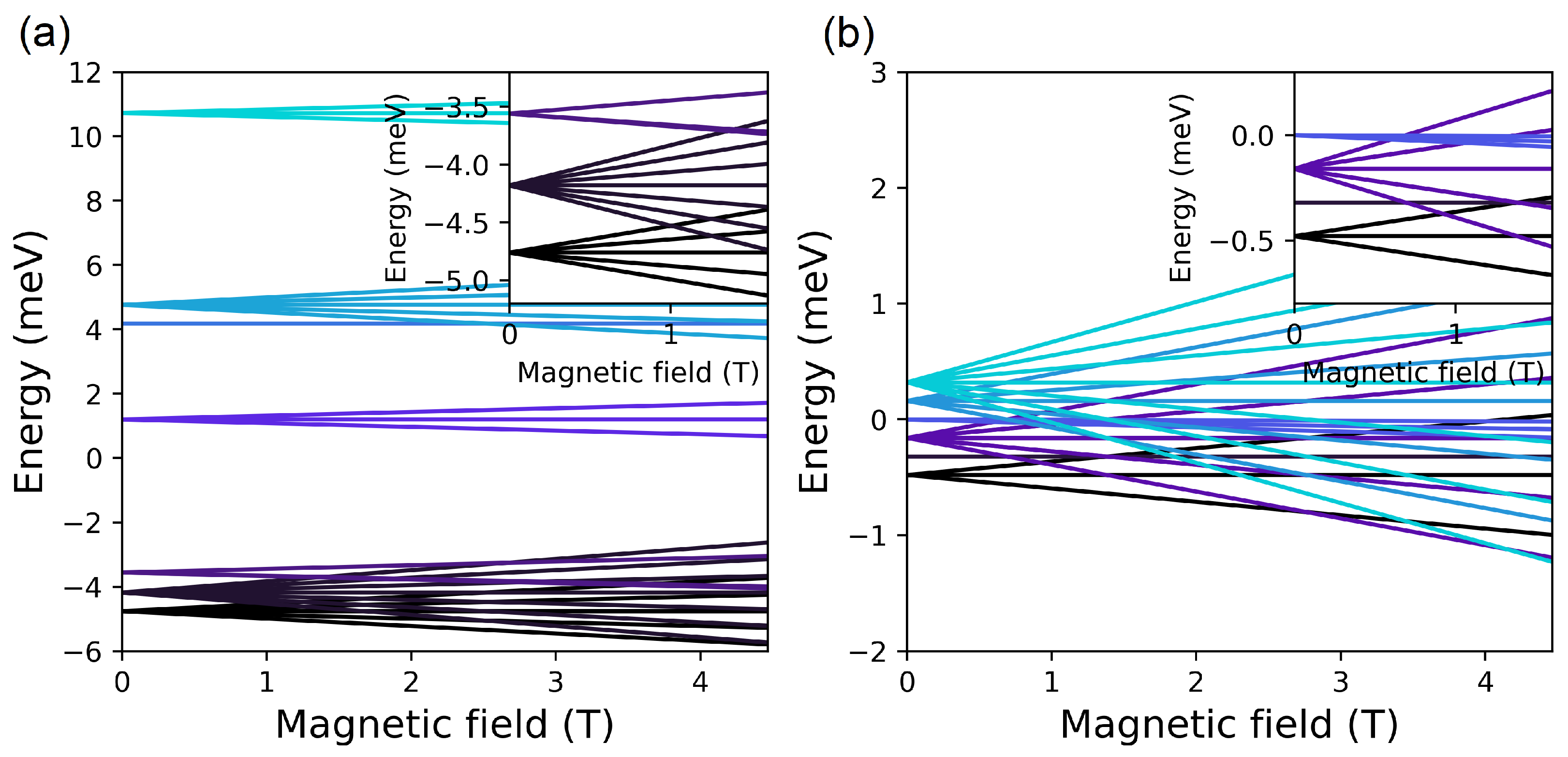
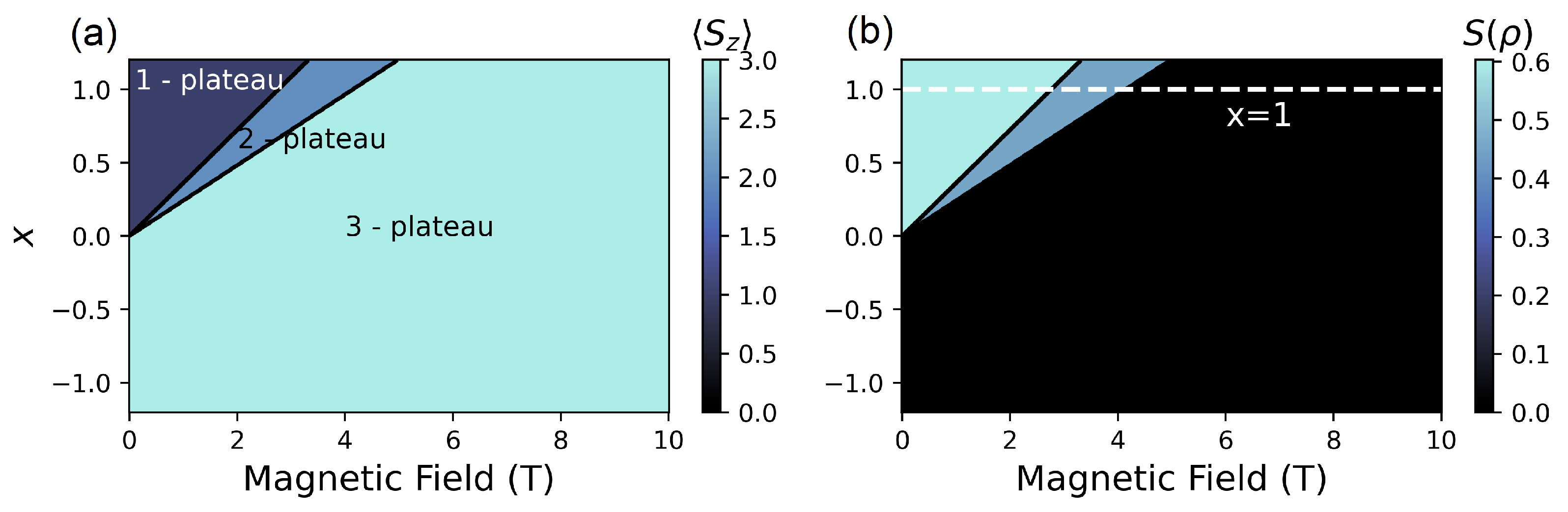
3.2. Two Coupled Molecules
4. Chain Magnets
4.1. Beyond Two SMMs
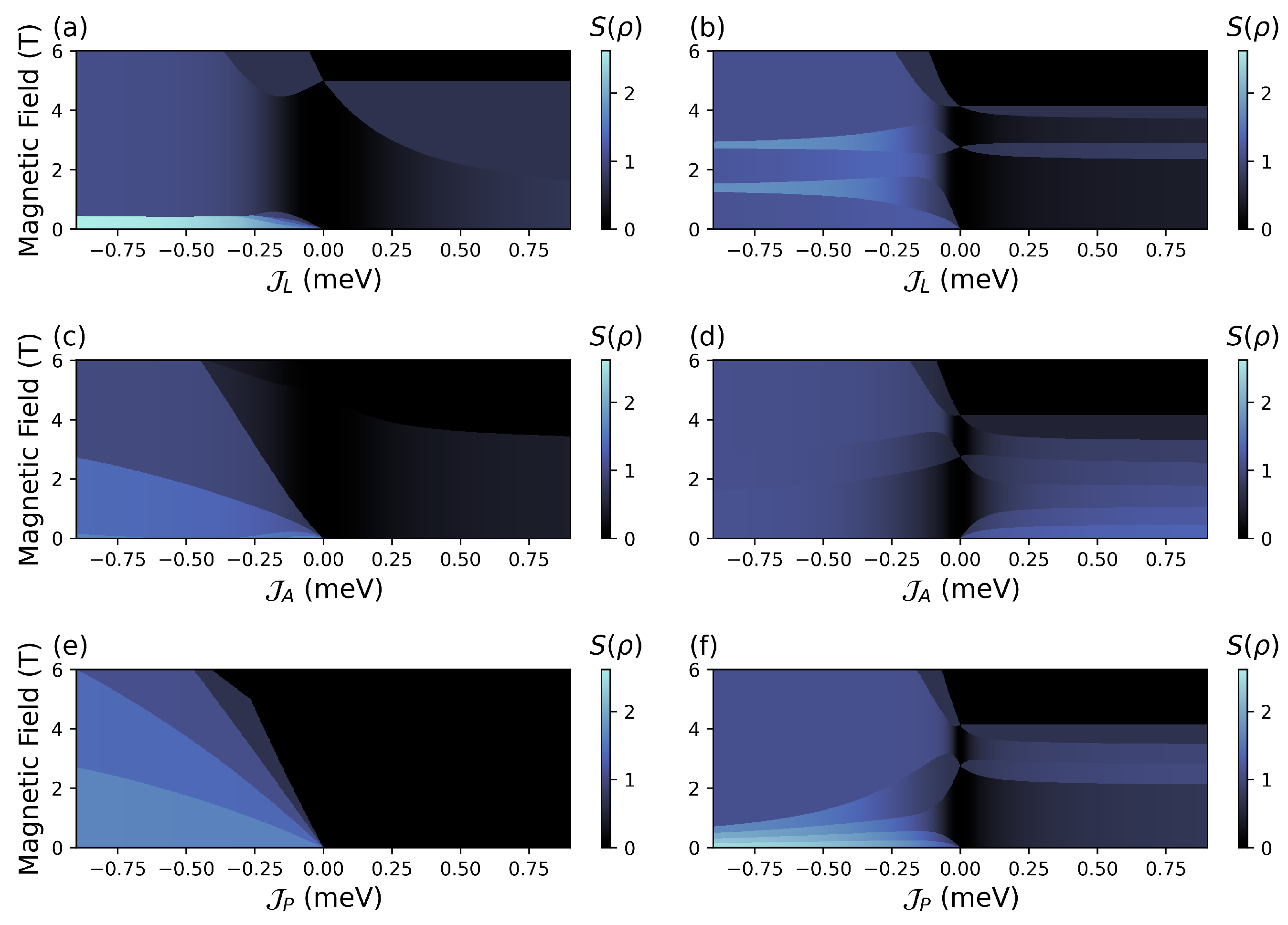
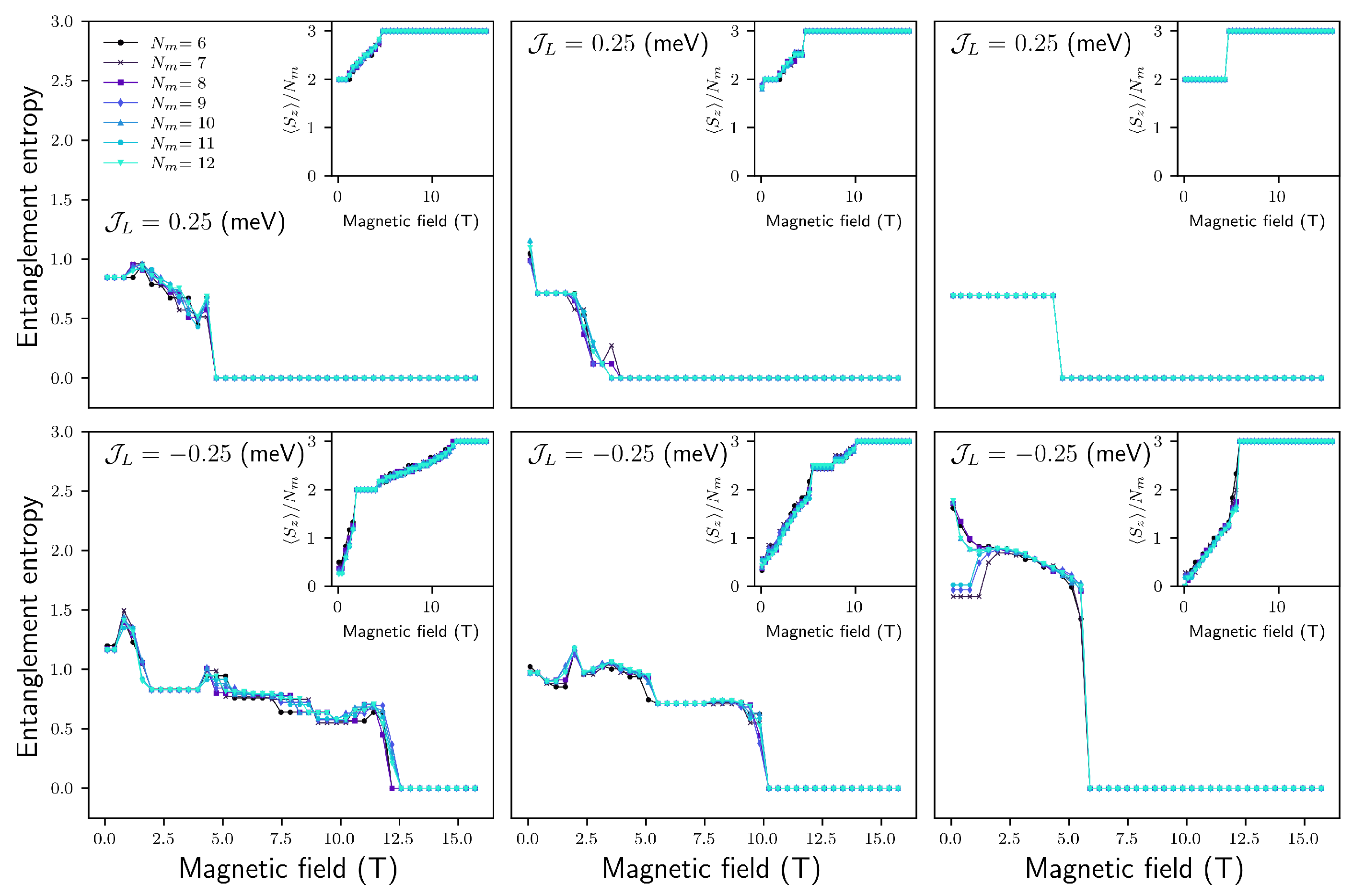
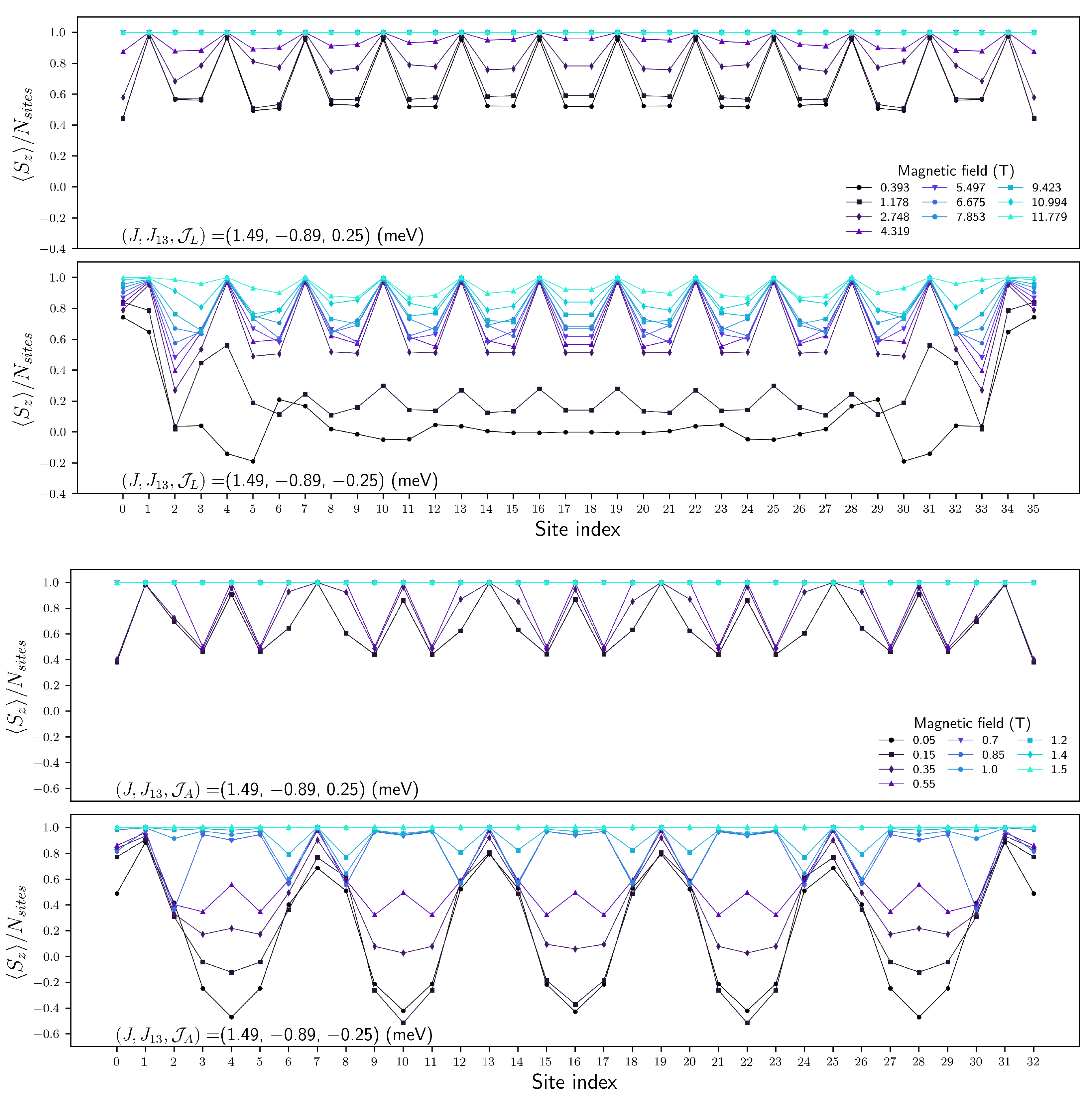
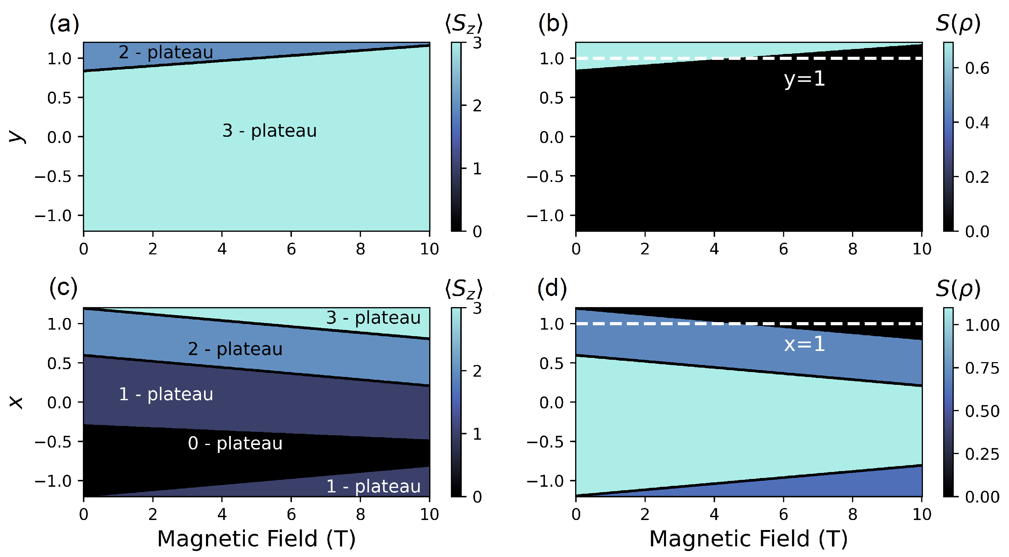
4.2. (, ) Quenching
4.2.1. Configuration
FM
AFM
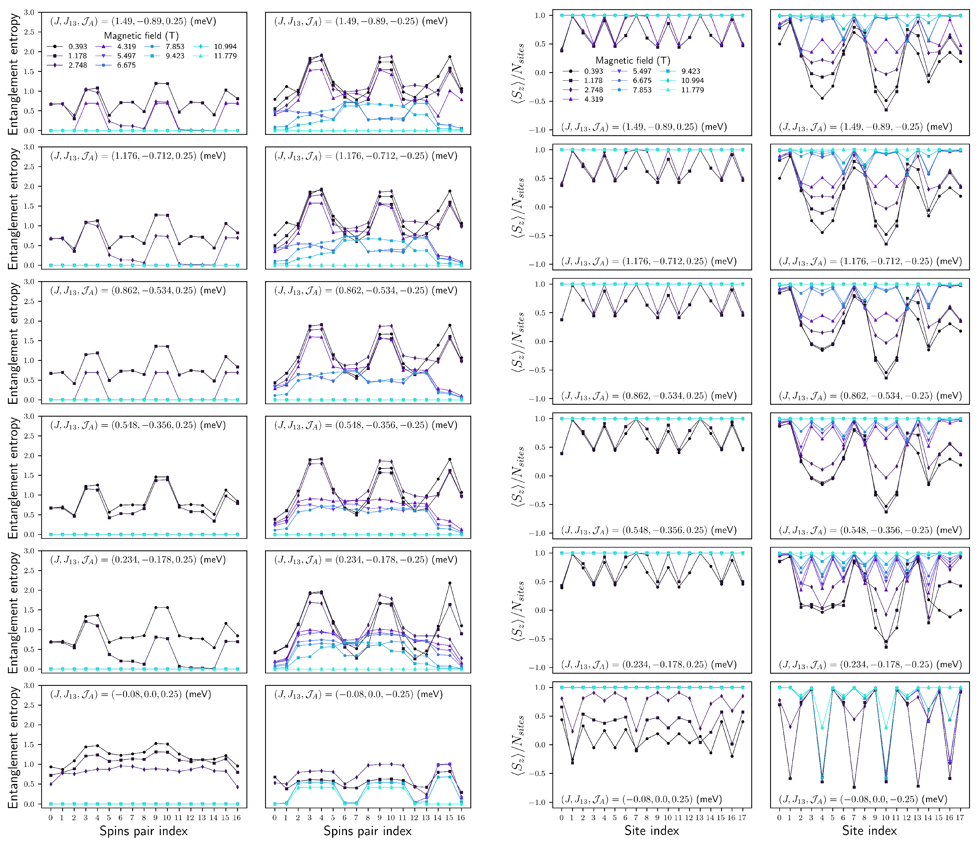
4.2.2. Configuration
FM
AFM
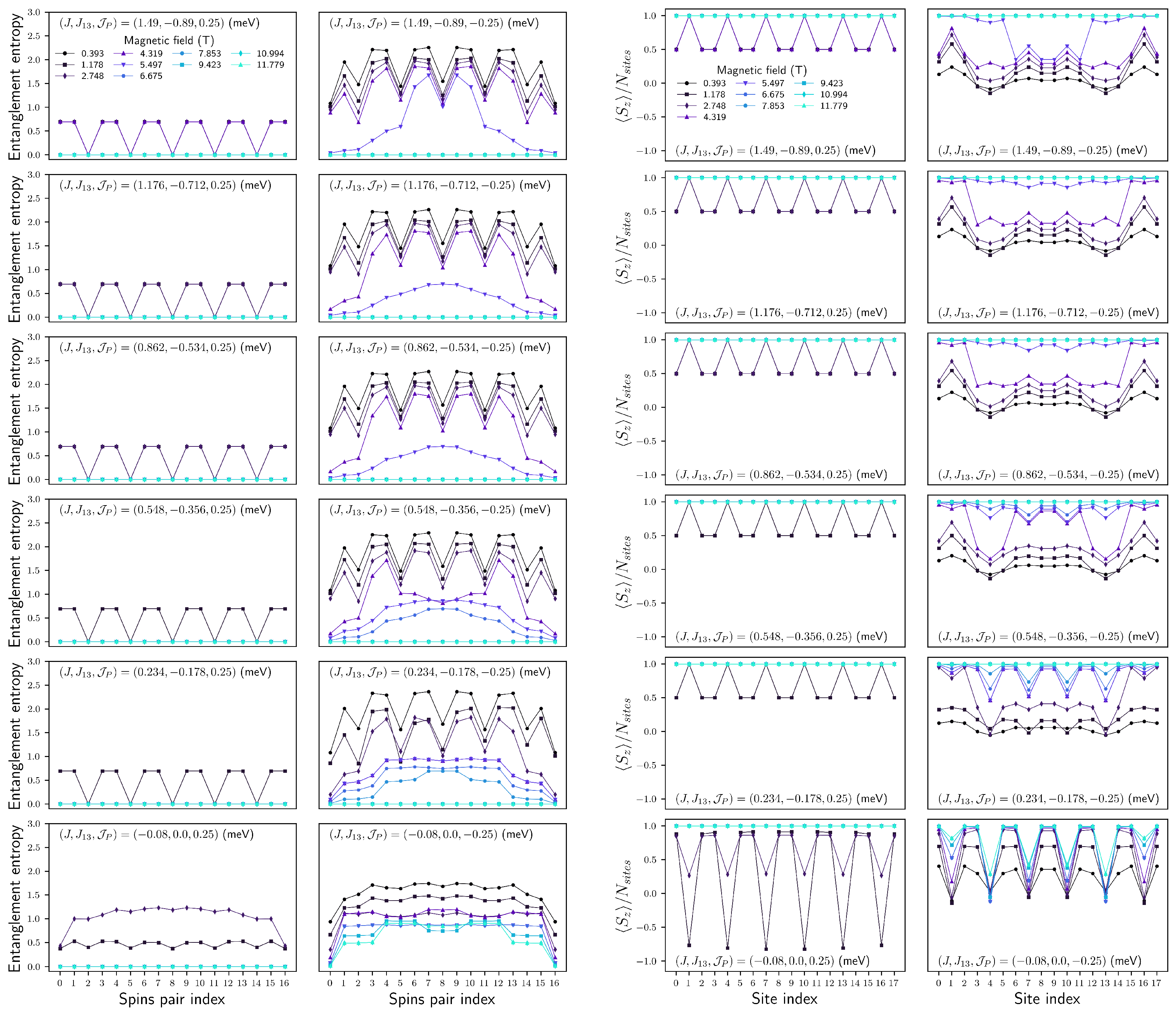
4.2.3. Configuration
FM
AFM
5. Conclusions
Author Contributions
Funding
Institutional Review Board Statement
Informed Consent Statement
Data Availability Statement
Conflicts of Interest
Abbreviations
| Ni(acac)2 | trimetric nickel(II) acetylacetonate |
| SMM | single-molecule magnet |
| nn | nearest-neighbor |
| L | linear |
| A | alternated |
| P | perpendicular |
| SWCNT | single-wall carbon nanotube |
| MPSs | Matrix Product States |
| DMRG | density-matrix renormalization group |
| Tenpy | Tensor Network Python |
| TDVPs | time-dependent variational principles |
| TEBDs | time-evolving block decimations |
| S | entanglement entropy or von Neumann’s |
| FM | ferromagnetism |
| AFM | antiferromagnetism |
Appendix A. Exact Solution for One and Two SMM

| Energy (meV) | State |
|---|---|
| Energy (meV) | State |
|---|---|


Appendix B. Entanglement of Chain Magnets
References
- Carretta, S.; Zueco, D.; Chiesa, A.; Gómez-León, A.; Luis, F. A perspective on scaling up quantum computation with molecular spins. Appl. Phys. Lett. 2021, 118, 240501. [Google Scholar] [CrossRef]
- Zabala-Lekuona, A.; Seco, J.M.; Colacio, E. Single-Molecule Magnets: From Mn12-ac to dysprosium metallocenes, a travel in time. Coord. Chem. Rev. 2021, 441, 213984. [Google Scholar] [CrossRef]
- Florez, J.M.; Vargas, P. Factorizing magnetic fields triggered by the Dzyaloshinskii–Moriya interaction: Application to magnetic trimers. J. Magn. Magn. Mater. 2012, 324, 83–89. [Google Scholar] [CrossRef]
- Ghirri, A.; Troiani, F.; Affronte, M. Quantum Computation with Molecular Nanomagnets: Achievements, Challenges, and New Trends. In Molecular Nanomagnets and Related Phenomena; Gao, S., Ed.; Springer: Berlin/Heidelberg, Germany, 2015; pp. 383–430. [Google Scholar] [CrossRef]
- Blachowicz, T.; Ehrmann, A. New Materials and Effects in Molecular Nanomagnets. Appl. Sci. 2021, 11, 7510. [Google Scholar] [CrossRef]
- Islam, R.; Ma, R.; Preiss, P.M.; Eric Tai, M.; Lukin, A.; Rispoli, M.; Greiner, M. Measuring entanglement entropy in a quantum many-body system. Nature 2015, 528, 77–83. [Google Scholar] [CrossRef] [PubMed]
- Bazhanov, D.I.; Sivkov, I.N.; Stepanyuk, V.S. Engineering of entanglement and spin state transfer via quantum chains of atomic spins at large separations. Sci. Rep. 2018, 8, 14118. [Google Scholar] [CrossRef] [PubMed]
- Ferrando-Soria, J.; Moreno Pineda, E.; Chiesa, A.; Fernandez, A.; Magee, S.A.; Carretta, S.; Santini, P.; Vitorica-Yrezabal, I.J.; Tuna, F.; Timco, G.A.; et al. A modular design of molecular qubits to implement universal quantum gates. Nat. Commun. 2016, 7, 11377. [Google Scholar] [CrossRef] [PubMed]
- Wu, W.H.; Wang, Y.Q.; Mi, H.L.; Xue, Q.X.; Shao, F.; Shen, F.; Yang, F.L. Magnetic relaxation in a Co(ii) chain complex: Synthesis, structure, and DFT computational coupling constant. CrystEngComm 2021, 23, 1398–1405. [Google Scholar] [CrossRef]
- Montenegro-Filho, R.R.; Silva-Júnior, E.J.P.; Coutinho-Filho, M.D. Ground-state phase diagram and thermodynamics of coupled trimer chains. Phys. Rev. B 2022, 105, 134423. [Google Scholar] [CrossRef]
- Sun, H.L.; Wang, Z.M.; Gao, S. Strategies towards single-chain magnets. Coord. Chem. Rev. 2010, 254, 1081–1100. [Google Scholar] [CrossRef]
- Cheng, J.Q.; Li, J.; Xiong, Z.; Wu, H.Q.; Sandvik, A.W.; Yao, D.X. Fractional and Composite Excitations of Antiferromagnetic Quantum Spin Trimer Chains. npj Quantum Mater. 2022, 7, 3. [Google Scholar] [CrossRef]
- Meng, X.; Shi, W.; Cheng, P. Magnetism in one-dimensional metal–nitronyl nitroxide radical system. Coord. Chem. Rev. 2019, 378, 134–150. [Google Scholar] [CrossRef]
- Tin, P. Haldane topological spin-1 chains in a planar metal-organic framework. Nat. Commun. 2023, 14, 5454. [Google Scholar] [CrossRef] [PubMed]
- Mellado, P. Intrinsic topological magnons in arrays of magnetic dipoles. Sci. Rep. 2022, 12, 1420. [Google Scholar] [CrossRef] [PubMed]
- Pouget, J.P. Spin-Peierls, Spin-Ladder and Kondo Coupling in Weakly Localized Quasi-1D Molecular Systems: An Overview. Magnetochemistry 2023, 9, 57. [Google Scholar] [CrossRef]
- Arian Zad, H.; Zoshki, A.; Ananikian, N.; Jaščur, M. Tomonaga-Luttinger Spin Liquid and Kosterlitz-Thouless Transition in the Spin-1/2 Branched Chains: The Study of Topological Phase Transition. Materials 2022, 15, 4183. [Google Scholar] [CrossRef] [PubMed]
- Mashiko, T.; Nomura, K. Phase transition of an SU(3) symmetric spin-1 chain. Phys. Rev. B 2021, 104, 155405. [Google Scholar] [CrossRef]
- Serwatka, T.; Melko, R.G.; Burkov, A.; Roy, P.N. Quantum Phase Transition in the One-Dimensional Water Chain. Phys. Rev. Lett. 2023, 130, 026201. [Google Scholar] [CrossRef]
- Baiardi, A.; Reiher, M. The density matrix renormalization group in chemistry and molecular physics: Recent developments and new challenges. J. Chem. Phys. 2020, 152, 040903. [Google Scholar] [CrossRef]
- Heveling, R.; Richter, J.; Schnack, J. Thermal density matrix renormalization group for highly frustrated quantum spin chains: A user perspective. J. Magn. Magn. Mater. 2019, 487, 165327. [Google Scholar] [CrossRef]
- Kim, J.; Kim, M.; Kawashima, N.; Han, J.H.; Lee, H.Y. Construction of variational matrix product states for the Heisenberg spin-1 chain. Phys. Rev. B 2020, 102, 085117. [Google Scholar] [CrossRef]
- Tilly, J.; Chen, H.; Cao, S.; Picozzi, D.; Setia, K.; Li, Y.; Grant, E.; Wossnig, L.; Rungger, I.; Booth, G.H.; et al. The Variational Quantum Eigensolver: A review of methods and best practices. Phys. Rep. 2022, 986, 1–128. [Google Scholar] [CrossRef]
- Castro, A.; García Carrizo, A.; Roca, S.; Zueco, D.; Luis, F. Optimal Control of Molecular Spin Qudits. Phys. Rev. Appl. 2022, 17, 064028. [Google Scholar] [CrossRef]
- Chizzini, M.; Crippa, L.; Chiesa, A.; Tacchino, F.; Petiziol, F.; Tavernelli, I.; Santini, P.; Carretta, S. Molecular nanomagnets with competing interactions as optimal units for qudit-based quantum computation. Phys. Rev. Res. 2022, 4, 043135. [Google Scholar] [CrossRef]
- Domanov, O.; Weschke, E.; Saito, T.; Peterlik, H.; Pichler, T.; Eisterer, M.; Shiozawa, H. Exchange coupling in a frustrated trimetric molecular magnet reversed by a 1D nano-confinement. Nanoscale 2019, 11, 10615–10621. [Google Scholar] [CrossRef]
- Bera, A.K.; Yusuf, S.M.; Saha, S.K.; Kumar, M.; Voneshen, D.; Skourski, Y.; Zvyagin, S.A. Emergent many-body composite excitations of interacting spin-1/2 trimers. Nat. Commun. 2022, 13, 6888. [Google Scholar] [CrossRef]
- Zhang, J.; Deng, Y.; Hu, X.; Chi, X.; Liu, J.; Chu, W.; Sun, L. Molecular Magnets Based on Graphenes and Carbon Nanotubes. Adv. Mater. 2019, 31, 1804917. [Google Scholar] [CrossRef]
- Villalva, J.; Develioglu, A.; Montenegro-Pohlhammer, N.; Sánchez-de Armas, R.; Gamonal, A.; Rial, E.; García-Hernández, M.; Ruiz-Gonzalez, L.; Costa, J.S.; Calzado, C.J.; et al. Spin-state-dependent electrical conductivity in single-walled carbon nanotubes encapsulating spin-crossover molecules. Nat. Commun. 2021, 12, 1578. [Google Scholar] [CrossRef]
- Florez, J.M.; Núñez, Á.; García, C.; Vargas, P. Magnetocaloric features of complex molecular magnets: The (Cr7Ni)2Cu molecular magnet and beyond. J. Magn. Magn. Mater. 2010, 322, 2810–2818. [Google Scholar] [CrossRef]
- Karl’ová, K.; Strečka, J.; Haniš, J.; Hagiwara, M. Insights into Nature of Magnetization Plateaus of a Nickel Complex [Ni4(μ-CO3)2(aetpy)8](ClO4)4 from a Spin-1 Heisenberg Diamond Cluster. Magnetochemistry 2020, 6, 59. [Google Scholar] [CrossRef]
- Park, K.; Yang, E.; Hendrickson, D. Electronic structure and magnetic anisotropy for nickel-based molecular magnets. J. Appl. Phys. 2005, 97, 10M522. [Google Scholar] [CrossRef]
- Ghannadan, A.; Karl’ová, K.; Strečka, J. On the Concurrent Bipartite Entanglement of a Spin-1 Heisenberg Diamond Cluster Developed for Tetranuclear Nickel Complexes. Magnetochemistry 2022, 8, 156. [Google Scholar] [CrossRef]
- Guo, F.; Bar, A.; Layfield, R. Main Group Chemistry at the Interface with Molecular Magnetism. Chem. Reviews 2019, 119, 8479–8505. [Google Scholar] [CrossRef]
- Bogani, L.; Wernsdorfer, W. Molecular spintronics using single-molecule magnets. Nat. Mater. 2008, 7, 155405. [Google Scholar] [CrossRef]
- Georgiev, M.; Chamati, H. Magnetization steps in the molecular magnet Ni4Mo12 revealed by complex exchange bridges. Phys. Rev. 2020, 101, 094427. [Google Scholar] [CrossRef]
- Florez, J.M.; Núñez, Á.S.; Vargas, P. Quenching points of dimeric single-molecule magnets: Exchange interaction effects. J. Magn. Magn. Mater. 2010, 322, 3623–3630. [Google Scholar] [CrossRef]
- Soto, R.; Martinez, G.; Baibich, M.N.; Florez, J.M.; Vargas, P. Metastable states in the triangular-lattice Ising model studied by Monte Carlo simulations: Application to the spin-chain compound Ca3Co2O6. Phys. Rev. B 2009, 79, 657. [Google Scholar] [CrossRef]
- Florez, J.M.; Vargas, P.; García, C.; Ross, C.A. Magnetic entropy change plateau in a geometrically frustrated layered system: FeCrAs-like iron-pnictide structure as a magnetocaloric prototype. J. Phys.-Condens. Matter 2013, 25, 226004. [Google Scholar] [CrossRef] [PubMed]
- Florez, J.M.; Negrete, O.A.; Vargas, P.; Ross, C.A. Geometrically frustrated Fe2P-like systems: Beyond the Fe-trimer approximation. J. Phys.-Condens. Matter 2015, 27, 1–10. [Google Scholar] [CrossRef]
- Ginsberg, A.P.; Martin, R.L.; Sherwood, R.C. Magnetic exchange in transition metal complexes. IV. Linear trimeric bis(acetylacetonato)nickel(II). Inorg. Chem. 1968, 7, 932–936. [Google Scholar] [CrossRef]
- Krichevsky, D.M.; Shi, L.; Baturin, V.S.; Rybkovsky, D.V.; Wu, Y.; Fedotov, P.V.; Obraztsova, E.D.; Kapralov, P.O.; Shilina, P.V.; Fung, K.; et al. Magnetic Nanoribbons with Embedded Cobalt Grown inside Single-Walled Carbon Nanotubes. Nanoscale 2022, 14, 1978–1989. [Google Scholar] [CrossRef]
- Kambe, K. On the Paramagnetic Susceptibilities of Some Polynuclear Complex Salts. J. Phys. Soc. Jpn. 1950, 5, 48–51. [Google Scholar] [CrossRef]
- Kharlamova, M.V.; Kramberger, C. Metallocene-Filled Single-Walled Carbon Nanotube Hybrids. Nanomaterials 2023, 13, 774. [Google Scholar] [CrossRef]
- Schollwöck, U. The Density-Matrix Renormalization Group in the Age of Matrix Product States. Ann. Phys. 2011, 326, 96–192. [Google Scholar] [CrossRef]
- Rausch, R.; Peschke, M.; Plorin, C.; Karrasch, C. Magnetic Properties of a Capped Kagome Molecule with 60 Quantum Spins. SciPost Phys. 2022, 12, 143. [Google Scholar] [CrossRef]
- Souza, F.; Veríssimo, L.M.; Strečka, J.; Lyra, M.L.; Pereira, M.S.S. Exact and Density Matrix Renormalization Group Studies of Two Mixed Spin-(1/2,5/2, 1/2) Branched-Chain Models Developed for a Heterotrimetallic Fe-Mn-Cu Coordination Polymer. Phys. Rev. B 2020, 102, 064414. [Google Scholar] [CrossRef]
- Haegeman, J.; Cirac, J.I.; Osborne, T.J.; Pižorn, I.; Verschelde, H.; Verstraete, F. Time-Dependent Variational Principle for Quantum Lattices. Phys. Rev. Lett. 2011, 107, 070601. [Google Scholar] [CrossRef] [PubMed]
- Haegeman, J.; Lubich, C.; Oseledets, I.; Vandereycken, B.; Verstraete, F. Unifying Time Evolution and Optimization with Matrix Product States. Phys. Rev. B 2016, 94, 165116. [Google Scholar] [CrossRef]
- Vidal, G. Efficient Simulation of One-Dimensional Quantum Many-Body Systems, Guifre Vidal. Phys. Rev. Lett. 2004, 93, 040502. [Google Scholar] [CrossRef]
- Hauschild, J.; Pollmann, F. Efficient Numerical Simulations with Tensor Networks: Tensor Network Python (TeNPy). SciPost Phys. Lect. Notes 2018, 5. [Google Scholar] [CrossRef]
- Um, J.; Park, H.; Hinrichsen, H. Entanglement versus mutual information in quantum spin chains. J. Stat. Mech. Theory Exp. 2012, 2012, P10026. [Google Scholar] [CrossRef]
- Amico, L.; Fazio, R.; Osterloh, A.; Vedral, V. Entanglement in many-body systems. Rev. Mod. Phys. 2008, 80, 517–576. [Google Scholar] [CrossRef]
- Scopa, S.; Calabrese, P.; Bastianello, A. Entanglement dynamics in confining spin chains. Phys. Rev. B 2022, 105, 125413. [Google Scholar] [CrossRef]
- Wei, K.X.; Ramanathan, C.; Cappellaro, P. Exploring Localization in Nuclear Spin Chains. Phys. Rev. Lett. 2018, 120, 070501. [Google Scholar] [CrossRef]
- Kam, C.F.; Chen, Y. Genuine Tripartite Entanglement as a Probe of Quantum Phase Transitions in a Spin-1 Heisenberg Chain with Single-Ion Anisotropy. Ann. Phys. 2022, 534, 2100342. [Google Scholar] [CrossRef]
- Scheie, A.; Laurell, P.; Samarakoon, A.M.; Lake, B.; Nagler, S.E.; Granroth, G.E.; Okamoto, S.; Alvarez, G.; Tennant, D.A. Witnessing entanglement in quantum magnets using neutron scattering. Phys. Rev. B 2021, 103, 224434. [Google Scholar] [CrossRef]
- Wootters, W.K. Entanglement of Formation of an Arbitrary State of Two Qubits. Phys. Rev. Lett. 1998, 80, 2245–2248. [Google Scholar] [CrossRef]
- Saguia, A.; Sarandy, M.S.; Boechat, B.; Continentino, M.A. Entanglement entropy in random quantum spin-S chains. Phys. Rev. A 2007, 75, 052329. [Google Scholar] [CrossRef]


Disclaimer/Publisher’s Note: The statements, opinions and data contained in all publications are solely those of the individual author(s) and contributor(s) and not of MDPI and/or the editor(s). MDPI and/or the editor(s) disclaim responsibility for any injury to people or property resulting from any ideas, methods, instructions or products referred to in the content. |
© 2024 by the authors. Licensee MDPI, Basel, Switzerland. This article is an open access article distributed under the terms and conditions of the Creative Commons Attribution (CC BY) license (https://creativecommons.org/licenses/by/4.0/).
Share and Cite
Norambuena Leiva, J.I.; Cortés Estay, E.A.; Suarez Morell, E.; Florez, J.M. On the Magnetization and Entanglement Plateaus in One-Dimensional Confined Molecular Magnets. Magnetochemistry 2024, 10, 10. https://doi.org/10.3390/magnetochemistry10020010
Norambuena Leiva JI, Cortés Estay EA, Suarez Morell E, Florez JM. On the Magnetization and Entanglement Plateaus in One-Dimensional Confined Molecular Magnets. Magnetochemistry. 2024; 10(2):10. https://doi.org/10.3390/magnetochemistry10020010
Chicago/Turabian StyleNorambuena Leiva, Javier I., Emilio A. Cortés Estay, Eric Suarez Morell, and Juan M. Florez. 2024. "On the Magnetization and Entanglement Plateaus in One-Dimensional Confined Molecular Magnets" Magnetochemistry 10, no. 2: 10. https://doi.org/10.3390/magnetochemistry10020010