Relationship between Structure and Zero-Field Splitting of Octahedral Nickel(II) Complexes with a Low-Symmetric Tetradentate Ligand

Abstract

Octahedral nickel(II) complexes are among the simplest systems that exhibit zero-field splitting by having two unpaired electrons. For the purpose of clarifying the relationship between structure and zero-field splitting in a low-symmetric system, distorted octahedral nickel(II) complexes were prepared with a tetradentate ligand, 2-[bis(2-methoxyethyl)aminomethyl]-4-nitrophenolate(1−) [(onp)⁻]. The complex [Ni(onp)(dmso)(H₂O)][BPh₄]·2dmso (1) (dmso = dimethyl sulfoxide) was characterized as a bulk sample by IR, elemental analysis, mass spectrometry, electronic spectra, and magnetic properties. The powder electronic spectral data were analyzed based on the angular overlap model to conclude that the spectra were typical of D₄-symmetric octahedral coordination geometry with a weak axial ligand field. Simultaneous analysis of the temperature-dependent susceptibility and field-dependent magnetization data yielded the positive axial zero-field splitting parameter D (H = g_uβS_uH_u + D[S_z² − S(S + 1)/3]), which was consistent with the weak axial ligand field. Single-crystal X-ray analysis revealed the crystal structures of [Ni(onp)(dmso)(H₂O)][BPh₄]·dmso (2) and [Ni(onp)(dmf)₂][BPh₄] (3) (dmf = N,N-dimethylformamide). The density functional theory (DFT) computations based on the crystal structures indicated the D₄-symmetric octahedral coordination geometries with weak axial ligand fields. This study also showed the importance of considering g-anisotropy in magnetic analysis, even if g-anisotropy is small.

1. Introduction

Octahedral nickel(II) complexes are among the simplest systems that exhibit zero-field splitting by having two unpaired electrons. (Please note that octahedral complexes do not necessarily have ideal octahedral symmetry [1], and zero-field splitting is affected by the slight symmetry reduction in the ligand field [2]). However, since the nickel(II) complex is an S = 1 non-Kramers system with an even number of unpaired electrons, high-frequency and high-field electron paramagnetic resonance (HFEPR) is required to observe the electron-paramagnetic-resonance (epr) signals to precisely determine the zero-field splitting parameters, D and E [3]. Here, the axial zero-field-splitting parameter D and the rhombic zero-field-splitting parameter E are defined as the phenomenological Hamiltonian H = g_uβS_uH_u + D[S_z² − S(S + 1)/3] + E(S_x² − S_y²) [4], which can also be derived from the formal spin-Hamiltonian [2]. Then, in the S = 1 system, the three originally degenerate microstates are split into −2D/3, D/3 − E, and D/3 + E energy levels without an external magnetic field. On the other hand, attempts to determine the zero-field-splitting parameters from magnetic data analysis have been successful [2,5], although not as accurate as HFEPR. The relationship between the coordination geometry around the nickel(II) ion and the sign of the axial zero-field splitting parameter D has been studied [2], and the result indicates that D is negative when the axial ligand field is strong (e_z > e_x,y) and positive when the axial ligand field is weak (e_z < e_x,y), where e_u represents the metal-ligand interaction in the u direction. Since the sign of the D parameter is related to magnetic anisotropy and the conditions for the single molecule magnets [2,6,7,8,9], even if there are exceptions [10], it is important to clarify the relationship between the sign of D and structure and to control the sign of D.

To determine the zero-field splitting parameters from the magnetic analysis, simultaneous fitting of the temperature dependence of magnetic susceptibility and the field dependence of magnetization is preferable [2]. For this purpose, it is, of course, essential to simulate magnetic susceptibility and magnetization. First, in the days when the cryomagnetic susceptibility was measured only down to about 5 K, it was not necessary to consider the effect of saturation by the applied magnetic field. However, now that it is common to measure magnetic susceptibility down to 2 K, a magnetic-field-dependent magnetic susceptibility equation is required to simulate the effect that the magnetic susceptibility is not proportional to the magnetic field at low temperatures. In addition, the eigenvalues are often series expanded with respect to the magnetic field to simplify the equation [2,4]; however, this should be avoided whenever possible, as it may reduce the accuracy of the calculation when |D| is small. The field-dependent magnetic susceptibility equation without using series expansion was reported for the S = 1 system [11]. In recent years, magnetization measurements have also become more common, and magnetization in the principal directions can be expressed in the same way as the magnetic field-dependent susceptibility equation. However, with powder samples, although the methodology is well established, it is not easy to express the powder average magnetization algebraically. In this study, we derive an algebraic expression for the exact powder average magnetization for the S = 1 system.

On the other hand, it is not easy to predict the sign of D when the symmetry of the ligand field around the central metal is not clear. (Please note that the symmetry of the ligand field [1] includes not only the position of the donor atoms but also their ligand-field strengths and the orientation of the donor π-orbitals.) In this study, nickel(II) complexes were prepared with a ligand, 2-[bis(2-methoxyethyl)aminomethyl]-4-nitrophenolate(1−) [(onp)⁻] (Figure 1), giving low-symmetric ligand fields to investigate the relationship between the structure and zero-field splitting parameters of low-symmetric nickel(II) complexes.

In the ligand (onp)⁻, the bis(2-methoxyethyl)aminomethyl motif is introduced at the 2-position of 4-nitrophenol, while the 4-chloro derivative was reported [12]. To our knowledge, the introduction of bis(2-methoxyethyl)aminomethyl motif into a phenol-based ligand was first conducted by Sakiyama to obtain 2,6-bis[bis(2-methoxyethyl)aminomethyl]-4-methylphenolate(1−) [(bomp)⁻] [13]. Subsequently, 4-chlorophenol and 4-nitrophenol derivatives were also synthesized [14]. In a series of syntheses, the more electron-withdrawing the 4-substituent is, the slower the reaction proceeds, but the cleaner the synthesis. Especially with 4-nitrophenol, which was used as the ligand in this study with a large electron-withdrawing property, the 2-substituted (onp)⁻ can be made easily and cleanly without 2,6-substituted (bonp)⁻ contamination. In synthesis, it is desirable to follow the raw materials and products in the reaction mixture chromatographically (e.g., by thin-layer chromatography) because slight differences in conditions can cause the reaction to proceed differently. Since formaldehyde, which has been used in past papers, is carcinogenic and volatile, it is better to use paraformaldehyde, which is not volatile. Great care should be taken when handling reactants.

2. Materials and Methods

2.1. Measurements

Elemental analyses (C, H, and N) were performed at the Elemental Analysis Service Centre of Kyushu University. Powder IR spectra were recorded on a Nicolet iS50 FTIR spectrometer and liquid IR spectra on a Jasco FT/IR-4000 using NaCl plates. Electrospray ionization (ESI) mass spectra were measured on a Waters Quattro micro-API mass spectrometer in mixed solvents (acetonitrile:dimethyl sulfoxide:H₂O = 4:1:1). Powder electronic spectra were measured on a Shimadzu UV-2600. Magnetic susceptibility measurements were performed with a Quantum Design MPMS-XL7 SQUID magnetometer. Temperature dependence of the susceptibility was measured in the temperature range from 1.9 to 300 K with a static field of 5 kOe. Field dependence of the magnetization was measured in the field range from 0 to 70 kOe at 2 K and 4 K. All data were corrected for the diamagnetism of the capsule and the samples by means of Pascal’s constants [15].

2.2. Materials

Methanol, ethanol, paraformaldehyde, p-nitrophenol, nickel(II) nitrate—water (1/6), N,N-dimethylformamide (dmf), dimethyl sulfoxide (dmso), and 2-propanol were supplied by Nacalai Tesque Inc., Kyoto, Japan. Bis(2-methoxyethyl)amine was supplied by Tokyo Chemical Industry Co., Ltd., Tokyo, Japan, Sodium tetraphenylborate was supplied by FUJIFILM Wako Pure Chemical Corporation, Osaka, Japan. H(onp) was prepared by refluxing the ethanolic solution (10 mL) of paraformaldehyde (1.51 g, 50.3 mmol), bis(2-methoxyethyl)amine (6.66 g, 50.0 mmol), and p-nitrophenol (7.01 g, 50.4 mmol) for 29 h (yield 12.02 g, 42.28 mmol, 84.6%), based on the literature method [16]. The IR spectra of H(onp) are shown in Figure S1.

2.3. Preparations

[Ni(onp)(dmso)(H₂O)][BPh₄]·2dmso 1. To a methanolic solution (20 mL) of Ni(NO₃)₂·6H₂O (0.31 g, 1.1 mmol) was added H(onp) (0.28 g, 0.98 mmol) and refluxed for 15 min. To this was added sodium tetraphenylborate (0.69 g, 2.0 mmol). After cooling, green precipitates were collected by filtration to obtain crude product (0.24 g). The crude product is considered to be mainly [Ni(onp)(H₂O)₂][BPh₄] with minor nitrate byproducts. Recrystallized from dmso/2-propanol to obtain green microcrystals. Yield 0.11 g (11%) (Found: C, 56.20; H, 6.25; N, 3.05; Ni, 7.1%. Calc. for C₄₃H₅₉BN₂NiO₉S₃: C, 56.50; H, 6.50; N, 3.05; Ni, 6.4%). Selected IR data [ṽ/cm^–1]: 3053–2914, 1595, 1479, 1298, 1284, 1259, 1076, 995, 949, 833, 823, 735, 706, 660, 611. ESI mass spectrum: m/z 341, [Ni(onp)]⁺; 419, [Ni(onp)(dmso)]⁺. IR spectra of the crude product and 1 are shown in Figure S1a and Figure S1b, respectively. The selected mass spectra for 1 are shown in Figures S3–S5.

2.4. Crystallography

Single-crystal X-ray diffraction data were obtained with a Rigaku XtaLAB AFC11 diffractometer with graphite-monochromated Mo Kα radiation (λ = 0.71073 Å). A single crystal was mounted with a cryoloop and flash-cooled with a cold N₂ gas stream. Data were processed using the CrysAlisPro 1.171.39.43a (Rigaku OD, 2018) software packages. The structure was solved by intrinsic phasing methods using the SHELXT 2018/2 (Sheldrick, 2018) [17] software packages and refined on F² (with all independent reflections) using the SHELXL 2018/3 (Sheldrick, 2018) [18] software packages. The non-hydrogen atoms were refined anisotropically, and hydrogen atoms, except for those of water molecules, were refined using the riding model. Hydrogen atoms for water molecules were located by Fourier difference map and fixed at the appropriate positions for hydrogen-bonding interactions during the refinement.

2.5. Computation

DFT computations were performed using the GAMESS [ver. 20 April 2017(R1)] program [19,20] on Fujitsu PRIMERGY CX2550/CX2560 M4 (ITO supercomputer system) at Kyushu University. Calculations were performed with LC-BOP/6-31G** [21] based on the restricted open-shell Hartree–Fock (ROHF). Angular overlap model (AOM) calculation was performed using the AOMX program on an Intel Celeron computer. Magnetic analyses were conducted by MagSaki(B) ver. W0.11.9 in MagSaki software series [22,23,24,25].

3. Results and Discussion

In this study, the nickel(II) complex [Ni(onp)(dmso)(H₂O)][BPh₄]·2dmso (1), obtained as a green powder, was characterized as a bulk sample by IR, elemental analysis, mass spectrometry, electronic spectra, and magnetic properties. The single-crystal sample [Ni(onp)(dmso)(H₂O)][BPh₄]·dmso (2), prepared similarly to 1, but slowly, was obtained only in small quantities and was used only for single-crystal X-ray structural analysis. The related single-crystal sample [Ni(onp)(dmf)₂][BPh₄] (3) was also used only for X-ray structural analysis.

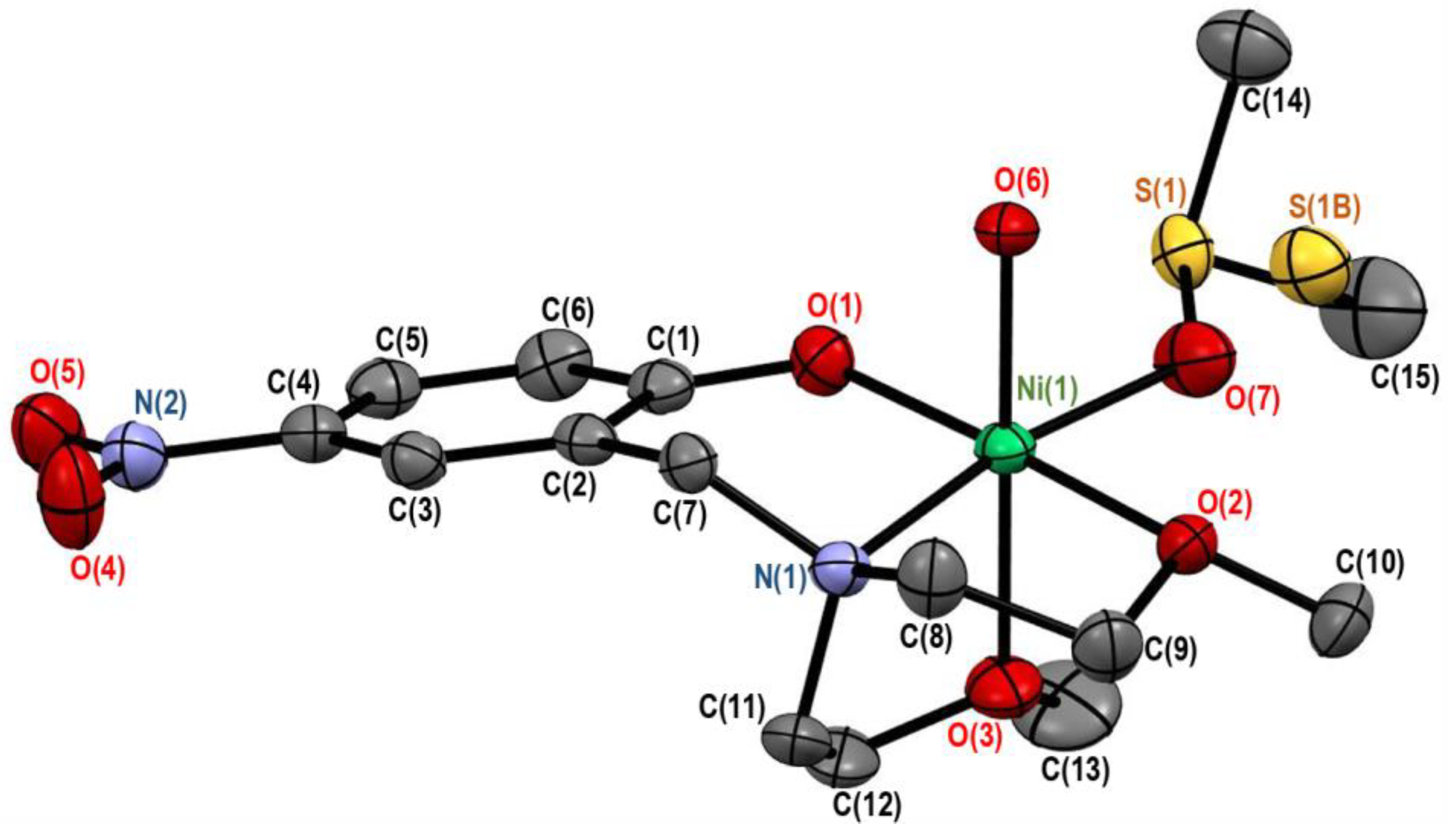
3.1. Crystal Structures of Complexes 2 and 3

Single crystals of [Ni(onp)(dmso)(H₂O)][BPh₄]·dmso (2) and [Ni(onp)(dmf)₂][BPh₄] (3), suitable for single-crystal X-ray analysis, were obtained by slow diffusion of 2-propanol into a dmso solution or a dmf solution of the crude product. Crystallographic data of 2 and 3 are summarized in

Table 1. Crystallographic data and refinement parameters of 2 and 3.

Compound	Complex 2	Complex 3
Empirical Formula	C41H53BN2NiO8S2	C43H53BN4NiO7
Formula Weight	835.49	807.41
Crystal system	monoclinic	monoclinic
Space group	P21/n	P21/c
a/Å	11.5855 (3)	12.6151 (2)
b/Å	16.3220 (4)	16.2543 (2)
c/Å	22.1213 (5)	20.7114 (3)
β/°	99.695 (2)	106.906 (2)
V/Å3	4123.36 (18)	4063.33 (11)
Z	4	4
Crystal Dimensions/mm	0.164 × 0.114 × 0.057	0.138 × 0.098 × 0.064
T/K	100	100
λ/Å	0.71073	0.71073
ρcalcd/g cm−3	1.346	1.320
µ/mm−1	0.625	0.533
F(000)	1768	1712
2θmax/◦	55	60
No. of Reflections Measured	28,549	60,987
No. of independent reflections	9416 (Rint = 0.0298)	10,822 (Rint = 0.0320)
Data/restraints/parameters	9416/3/518	10,822/0/511
R1 (I > 2.00σ(I)) 1	0.0409	0.0297
wR2 (All reflections) 2	0.1093	0.0852
Goodness of Fit Indicator	1.045	1.044
Highest peak, deepest hole/e Å−3	1.001, −0.539	0.413, −0.416
CCDC deposition number	2335894	2335893

¹ R1 = Σ||Fo| − |Fc||/Σ|Fo|, ² wR2 = [Σ(w(Fo² − Fc²)²)/Σw(Fo²)²]^1/2.

with the Cambridge Crystallographic Data Centre (CCDC) deposition numbers.

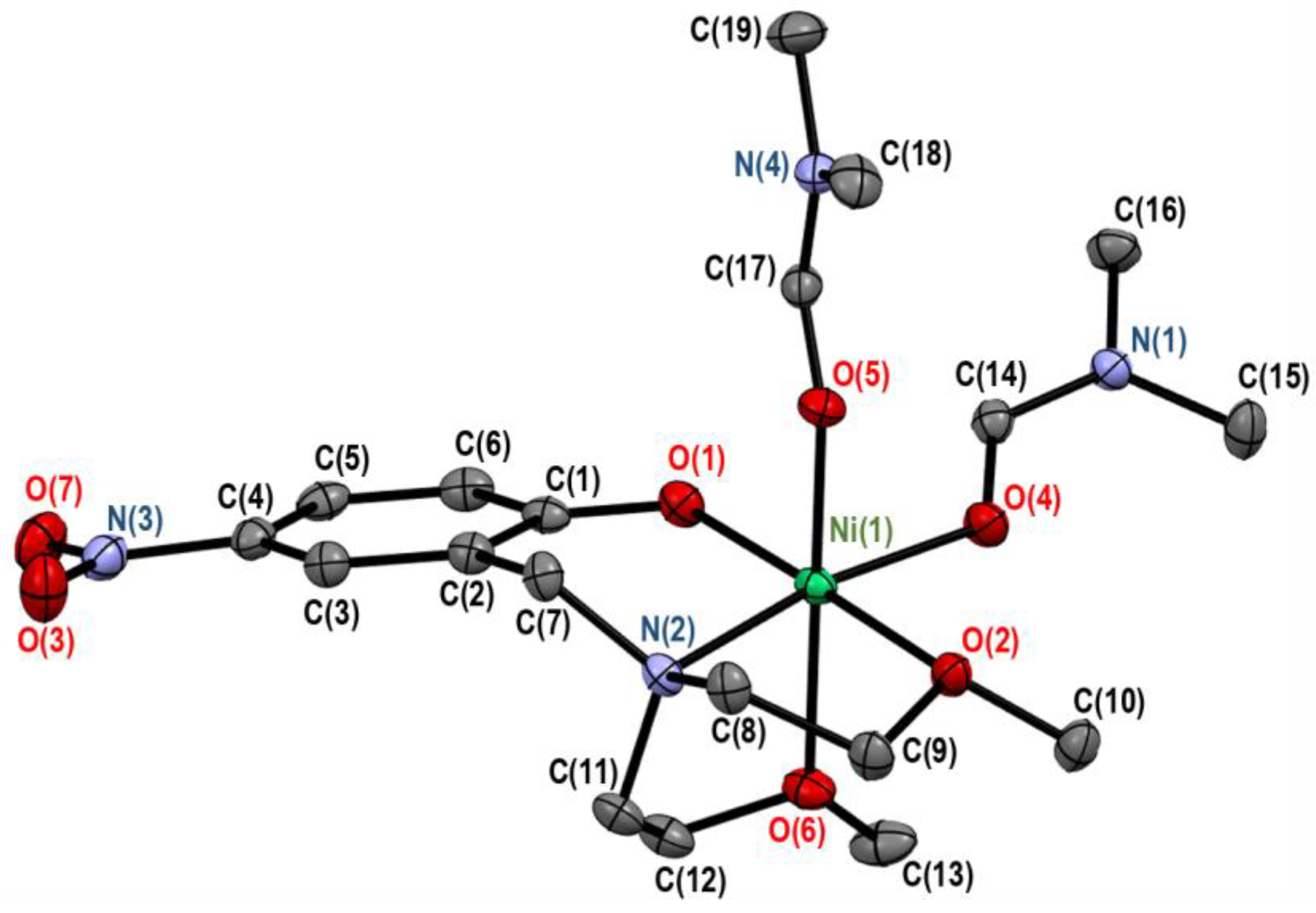
3.1.1. Crystal Structure of [Ni(onp)(dmso)(H₂O)][BPh₄]·dmso (2)

Crystals of 2 consists of [Ni(onp)(dmso)(H₂O)]⁺ complex cations and tetraphenylborate anions ([BPh₄]⁻) in a 1:1 molar ratio. The crystal structure of [Ni(onp)(dmso)(H₂O)]⁺ complex cation is depicted in Figure 2. The selected bond distances and angles are summarized in

Table 2. Selected bond distances for 2.

Atom–Atom	Distance/Å	Atom–Atom	Distance/Å
Ni(1)–O(1)	1.9957(14)	Ni(1)–O(2)	2.1199 (14)
Ni(1)–O(3)	2.1121(15)	Ni(1)–O(6)	2.0708 (14)
Ni(1)–O(7)	2.0261(16)	Ni(1)–N(1)	2.0583 (17)

and

Table 3. Selected bond angles for 2.

Atom–Atom–Atom	Angle/°	Atom–Atom–Atom	Angle/°
O(1)–Ni(1)–O(2)	176.09 (6)	O(1)–Ni(1)–O(3)	93.37 (6)
O(1)–Ni(1)–O(6)	91.60 (6)	O(1)–Ni(1)–O(7)	95.30 (7)
O(1)–Ni(1)–N(1)	93.15 (6)	O(2)–Ni(1)–O(3)	87.02 (6)
O(2)–Ni(1)–O(6)	87.68 (6)	O(2)–Ni(1)–O(7)	88.54 (7)
O(2)–Ni(1)–N(1)	83.07 (6)	O(3)–Ni(1)–O(6)	172.88 (6)
O(3)–Ni(1)–O(7)	94.28 (7)	O(3)–Ni(1)–N(1)	80.59 (6)
O(6)–Ni(1)–O(7)	90.33 (6)	O(6)–Ni(1)–N(1)	94.06 (6)
O(7)–Ni(1)–N(1)	170.36 (7)

. In the complex cation, the (onp)⁻ ligand worked as a tetradentate ligand, and the dmso and aqua ligands worked as monodentate ligands. The dmso ligand coordinated to the central nickel(II) ion through the oxygen atom, and the sulfur atom was disordered [occupancies: S(1), 0.7757(19); S(1B), 0.2243(19)]. This is a typical phenomenon for an oxygen-coordinating dmso ligand due to the sulfur inversion [26,27]. The coordination geometry around the central nickel(II) ion was octahedral with NO₅ donor atoms. The bond distances around the nickel(II) ion are normal for the related nickel(II) complexes [28,29], but the coordination geometry was slightly elongated along the O(3)-Ni(1)-O(6) direction. When the (onp)⁻ ligand acts as a tetradentate ligand in an octahedral nickel(II) complex, the remaining two vacant sites should be in the cis-positions due to the steric requirement of the (onp)⁻ ligand. Furthermore, the space of the vacant sites is not enough for the coordination of two dmso ligands. Therefore, the coordination of the aqua ligand with the dmso ligand is considered inevitable.

3.1.2. Crystal Structure of [Ni(onp)(dmf)₂][BPh₄] (3)

Crystals of 3 consist of [Ni(onp)(dmf)₂]⁺ complex cations and [BPh₄]⁻ anions in a 1:1 molar ratio. The crystal structure of [Ni(onp)(dmf)₂]⁺ complex cation is shown in Figure 3. The selected bond distances and angles are summarized in

Table 4. Selected bond distances for 3.

Atom–Atom	Distance/Å	Atom–Atom	Distance/Å
Ni(1)–O(1)	1.9906 (8)	Ni(1)–O(2)	2.1330 (8)
Ni(1)–O(4)	2.0295 (8)	Ni(1)–O(5)	2.0709 (8)
Ni(1)–O(6)	2.1240 (8)	Ni(1)–N(2)	2.0643 (9)

and

Table 5. Selected bond angles for 3.

Atom–Atom–Atom	Angle/°	Atom–Atom–Atom	Angle/°
O(1)–Ni(1)–O(2)	177.10 (3)	O(1)–Ni(1)–O(4)	93.97 (3)
O(1)–Ni(1)–O(5)	93.28 (3)	O(1)–Ni(1)–O(6)	94.85 (3)
O(1)–Ni(1)–N(2)	94.22 (3)	O(2)–Ni(1)–O(4)	88.85 (3)
O(2)–Ni(1)–O(5)	86.00 (3)	O(2)–Ni(1)–O(6)	85.53 (3)
O(2)–Ni(1)–N(2)	83.01(3)	O(4)–Ni(1)–O(5)	91.61 (3)
O(4)–Ni(1)–O(6)	94.96 (3)	O(4)–Ni(1)–N(2)	170.58 (3)
O(5)–Ni(1)–O(6)	169.17 (3)	O(5)–Ni(1)–N(2)	92.55 (3)
O(6)–Ni(1)–N(2)	79.72 (3)

. In the complex cation, the (onp)⁻ ligand worked as a tetradentate ligand, and the two dmf ligands worked as monodentate ligands. The coordination geometry around the central nickel(II) ion was octahedral with NO₅ donor atoms. The bond distances around the nickel(II) ion are normal for the related nickel(II) complexes [28,29], but the coordination geometry is slightly elongated along the O(5)-Ni(1)-O(6) direction. In both 2 and 3, the distortion patterns for the octahedral geometry are very similar to each other, although the exogenous ligands are different. In the case of the dmf ligand, the space required for coordination is smaller than that of the dmso ligand, allowing two dmf ligands to bind to the central nickel(II) ion.

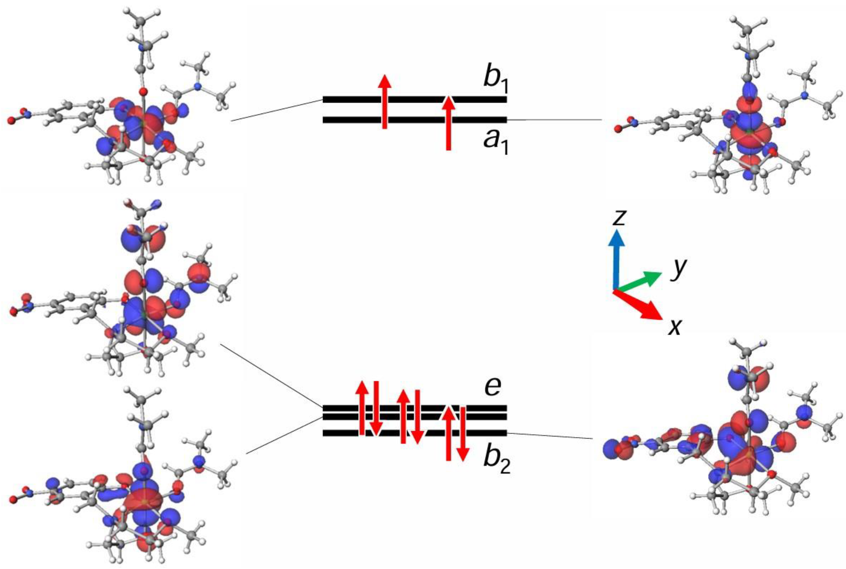
3.2. Density Functional Theory (DFT) Computations for Complexes 2 and 3

To gain a better understanding of the ground state, density functional theory (DFT) computations were conducted for the crystallographically identified complex cations in 2 and 3. The energy diagrams and d-orbital-related molecular orbitals for 2 and 3 are shown in Figure 4 and Figure 5, respectively. The results for the two complex cations were very similar, and we will first discuss the [Ni(onp)(dmso)(H₂O)]⁺ complex cation in 2. Judging from the splitting pattern of the five d-orbital-related molecular orbitals, the coordination geometry can be well approximated as the D₄ rotation group. (Please note that the D₄ rotation group [30] is a subgroup of the D_4h point group but is defined as a group considering only rotation operations. The D₄ rotation group is the simplest group suitable for reproducing the splitting pattern and the phase of the orbitals based on the coordination geometry). The five orbitals can be approximately assigned to b₂, e, a₁, and b₁ from the lower energy, where the e orbital set is doubly degenerate. The three lower orbitals (b₂ and e) are each filled with two electrons, but the two upper orbitals (a₁ and b₁) are each singly occupied and are magnetic orbitals. One important point is that the b₁ (d_x²_−y²) orbital is above the a₁ (d_z²) orbital in the magnetic orbitals, indicating that the ligand field in the z direction is weaker than those in the x and y directions, which is consistent with the elongation along the O(3)-Ni(1)-O(6) direction (z direction) in the crystal structure. The other important point is the degenerate e orbital set. Although not completely degenerate due to the mixing of the ligand orbitals, the spread of the two orbitals shows linear combinations of the d_xz and d_yz orbitals. This indicates that the magnitudes of the ligand fields in the x and y directions are approximately the same. The characteristics of the energy diagram and molecular orbitals for 3 are basically the same as those of 2. The ligand field in the z direction is weaker than those in the x and y directions, but the ligand fields in the x and y directions are approximately the same.

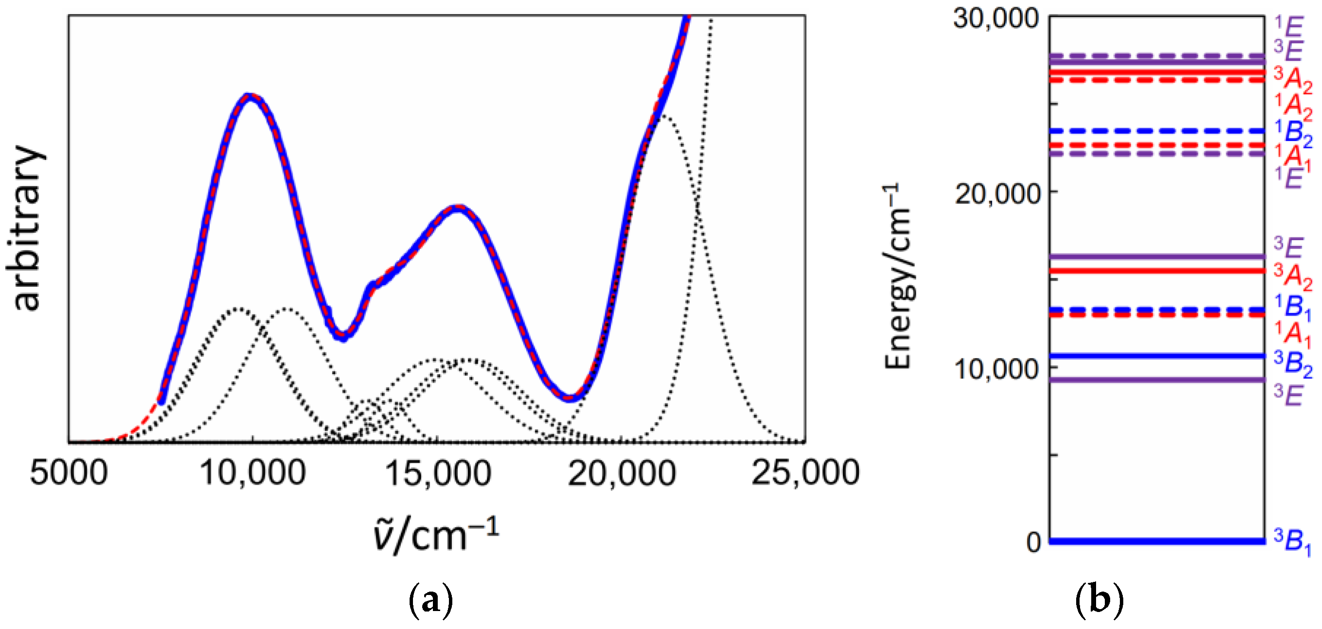
3.3. Electronic Spectra of 1

The powder electronic spectra were measured for 1 by the diffuse reflection method at room temperature, as shown in Figure 6a. The spectra were typical of an octahedral nickel(II) complex with two spin-allowed bands from near-infrared to visible range. Assuming the O symmetry, the first spin-allowed band at around 10,000 cm⁻¹ was assigned to ³A₂(³F) → ³T₂(³F), a small shoulder band at around 13,000 cm⁻¹ to ³A₂ → ¹E(¹D), the second spin-allowed band at around 16,000 cm⁻¹ to ³A₂ → ³T₁(³F). The expected third spin-allowed band [³A₂ → ³T₁(³P)] was hidden in the bands originating from the ligand. Focusing on the band shapes of the first and the second spin-allowed bands, the first band is slightly inclined toward the lower energy (the lower-energy side is steeper than the other), but the second band is slightly inclined toward the higher energy (higher energy side is steeper than the other). This feature was clearly reaffirmed by Gaussian curve fitting, assuming three spectral components of equal height and width. (Please note that while these restrictions may not be strictly correct, the ability to uniquely determine the solution in the initial process of fitting is an advantage.) The obtained spectral components are also shown in Figure 6a, and the sum of the spectral components fits the observed data very well. This splitting pattern is typical of tetragonally elongated octahedral geometry with a weak axial ligand field [31].

Next, angular overlap model (AOM) calculations were performed assuming D₄ symmetry to reproduce the obtained spectral components. The best-fitting parameter set was obtained as (B, C, e_σ,ax, e_σ,eq) = (920 cm⁻¹, 3200 cm⁻¹, 2690 cm⁻¹, 3550 cm⁻¹), where B and C are the Racah parameters, and e_σ,ax and e_σ,eq are the axial (z direction) and the equatorial (x, y direction) AOM parameters, corresponding to the metal-ligand σ interactions [1]. The π interactions were not considered in the calculation. The resulting energy levels of the states are shown in Figure 6b, together with the assignment of states in the D₄ symmetry. The AOM parameters obtained from the spectral analysis show that the ligand field of complex 1 is D₄ symmetric and axially weak (e_σ,ax < e_σ,eq), which is consistent with the DFT results for 2 and 3. The D₄ symmetry and the axially weak ligand field around the central nickel(II) ion may be due to the nature of the (omp)⁻ ligand. Furthermore, it is reasonable to assume that the structure of the complex cation in 1 is the same as that in 2 since the steric requirements of the (omp)⁻ ligand prevent the two dmso ligands from binding to the nickel(II) ion, as discussed in Section 3.1.1.

3.4. Theory and Magnetic Equations

Prior to magnetic analysis, the equations necessary for magnetic analysis are organized and summarized here. In particular, closed-form algebraic equations describing the magnetization in any field direction in the S = 1 system will be derived in this study. This allows the powder magnetization to be expressed in terms of algebraic equations.

In molecular magnetism, the following procedure is generally used to simulate magnetization and magnetic susceptibility [4,32]. First, the Hamiltonian is defined, and then the energy matrix is obtained from the Hamiltonian and the appropriate set of basis functions. Solving the secular equation yields the energy of the microstates as eigenvalues. Furthermore, partial differentiation of the obtained eigenvalues with respect to the magnetic field yields the microscopic magnetization of the microstates. Then, by considering the Boltzmann distribution, the equations for magnetization and magnetic susceptibility can be obtained. In the process of solving the secular equation to obtain eigenvalues, the dimension of the matrix is often too large to obtain an exact solution, but in the present S = 1 system, the dimension of the matrix is only 3 × 3, so the exact solution can be obtained algebraically.

Since powder samples were used for magnetic measurements, the powder average in Equation (1) [2,4] must be used for simulations in magnetic susceptibility data analysis for magnetically anisotropic compounds.

$${\chi }_{\mathrm{a}\mathrm{v}}=\frac{1}{4\pi }{\int }_0^{\pi }{\int }_0^{2\pi }\chi \left(\theta ,\phi \right)\sin \theta d\phi d\theta$$

(1)

However, since the magnetic susceptibility in weak magnetic fields is additive, the powder average is the same as the arithmetic average. When the symmetry is axial, the susceptibility is written as in Equation (2), which is the same as Equation (A1) in Appendix A.

$${\chi }_{\mathrm{a}\mathrm{v}}=\frac{{\chi }_z+2{\chi }_x}{3}$$

(2)

To calculate the principal magnetic susceptibilities χ_z and χ_x in Equation (2), previously derived Equations (A2) and (A3) [11] in Appendix A are useful for the S = 1 system. Considering the axial anisotropic g-factors (g_z and g_x), the axial zero-field splitting (D), temperature-independent paramagnetism (χ_tip,z and χ_tip,x), and intermolecular interaction (zJ), the atomic magnetic susceptibility, χ_A, and its components are expressed as Equations (A4)–(A7) [11] in Appendix A.

The problem here is the magnetization with anisotropy. While the principal magnetization (M_x, M_y, and M_z) can be easily expressed, the powder average can be expressed as the arithmetic average of the principal magnetization only in weak magnetic fields where the magnetization is proportional to the field. The principal magnetization M_z and M_x in axial symmetry can be expressed as Equations (A8) and (A9) in Appendix B. The powder average magnetization required for magnetization simulation in high magnetic fields can be written as in Equation (3). In Equation (3), the function M(θ, φ) represents the magnetization in the u(θ, φ) direction of the polar coordinates when the magnetic field is applied along the direction u(θ, φ). To calculate the exact powder average of the magnetization, we first need to express the function M(θ, φ).

$$M_{\mathrm{a}\mathrm{v}}=\frac{1}{4\pi }{\int }_0^{\pi }{\int }_0^{2\pi }M\left(\theta ,\phi \right)\sin \theta d\phi d\theta$$

(3)

In the axial symmetry, the Hamiltonian H = g_uβS_uH_u + D[S_z² − S(S + 1)/3] can be rewritten as H = g_zβS_zH_ucosθ + g_xβS_xH_usinθ + D[S_z² − S(S + 1)/3] [33], and the energy matrix can be written below. Here, $|1⟩$, $|0⟩$, and $|-1⟩$ represent the microstates of the S = 1 state.

$\left|1\right.⟩$	$\left|0\right.⟩$	$\left|-1\right.⟩$
gz β Hu cosθ + D/3	$\left(\sqrt{2}/2\right)$gx β Hu sinθ	0
$\left(\sqrt{2}/2\right)$gx β Hu sinθ	−2D/3	$\left(\sqrt{2}/2\right)$gx β Hu sinθ
0	$\left(\sqrt{2}/2\right)$gx β Hu sinθ	−gz β Hu cosθ + D/3

Fortunately, this matrix can be solved algebraically to obtain three eigenvalues, E_u,1, E_u,2, and E_u,3, as closed-form expressions. Hence, the eigenvalues are partially differentiable with respect to the magnetic field, and the microscopic magnetization [μ_u,n = −∂E_u,n⁄∂H_u (n = 1, 2, 3)] can also be expressed algebraically. Thus, in axial symmetry, the magnetization in any u(θ) direction, M_θ(θ), can be expressed as a closed-form algebraic expression. The obtained expressions are given as Equations (A10)–(A27) in Appendix C, i.e., the magnetic anisotropy is expressed as the θ-dependent (orientation-dependent) magnetization affected by the zero-field splitting (D) and g-anisotropy.

Now the function M(θ, φ) in Equation (3) has been obtained as the function M_θ(θ) in the axial symmetry (Equation (A27)), and the powder average can be approximated, using numerical integration [11,34]. In Equation (4), exact integration is conducted with respect to φ, and numerical integration is conducted with respect to θ in 1.0° steps from 0.5° to 89.5°. This equation gives a highly accurate approximation of the powder average. However, if more precision is needed, Equation (5) can be used instead of Equation (4), for example.

$$M_{\mathrm{a}\mathrm{v}}\approx \sum _{j=1}^{90}{M}_{\theta }\left(j-0.5\right)\left[\cos \left(\frac{\left(j-1\right)\pi }{180}\right)-\cos \left(\frac{j \pi }{180}\right)\right]$$

(4)

$$M_{av}\approx \sum _{j=1}^{900}{M}_{\theta }\left(j/10-0.05\right)\left[\cos \left(\frac{\left(j-1\right)\pi }{1800}\right)-\cos \left(\frac{j \pi }{1800}\right)\right]$$

(5)

3.5. Magnetic Properties of Complex 1

As discussed in Section 3.3, the structure of the complex cation in 1 is considered to be the same as that in 2. Temperature dependence of magnetic susceptibility (χ_A) and field dependence of magnetization (M) were measured for 1. The χ_AT versus T and the M versus H plots for 1 is shown in Figure 7. The χ_AT value at 300 K was 1.43 cm³ K mol⁻¹, which was slightly larger than the spin-only value (1.00 cm³ K mol⁻¹) for the S = 1 system assuming g = 2. When decreasing the temperature, the χ_AT value was almost constant, but below 15 K, the value dropped to show the minimum (0.62 cm³ K mol^–1) at 1.9 K. This dropping behavior can be explained by very small antiferromagnetic intermolecular interaction, but also by the zero-field splitting of the ground state. As the magnetic field increases, the M/Nβ value is going to saturate to ~2.0, which is consistent with the S = 1 system.

In this study, the field-dependent magnetic susceptibility equations (Equations (A1)–(A7) in Appendix A) [11] were used for simulating magnetic susceptibility, and magnetization equations (Equations (A10)–(A27) in Appendix C and Equation (4)) for simulating magnetization, considering the axial anisotropic g-factors (g_z and g_x), the axial zero-field splitting (D), temperature-independent paramagnetism (χ_tip), and intermolecular interaction (zJ). In the magnetic analysis, the χ_tip-anisotropy was not considered.

As the result of simultaneous analysis, the best-fitting parameter set was obtained as (g_z, g_x, D, zJ, χ_tip) = (2.13, 2.31, +5.9 cm⁻¹, −0.70 cm⁻¹, 534 × 10⁻⁶ cm³ mol⁻¹) at 5 kOe. When χ_AT decreases at very low temperatures (below 15 K), separating zJ and D is not easy, but it should be possible to separate them because their temperature dependencies are generally different. This time, we were able to find the best combination of zJ and D by simultaneous fitting of magnetic susceptibility and magnetization due to the fact that the difference between the theoretical magnetization curves for 2 K and 4 K is larger for larger −zJ. Determining the sign of D is also difficult, but reversing the sign of D worsens the fitting of the theoretical magnetization curve to the measured values. The positive D value suggests that the axial ligand field is weaker than the equatorial ligand field [2], which is concordant with the result of powder electronic spectra for 1 (Section 3.3) and also with the DFT result for 2, whose cation structure is considered to be the same (Section 3.2). Although it is difficult to obtain precise g-values from magnetic data, considering g-anisotropy improves the fitting of magnetization in the high-field region. The resulting anisotropic g-factor relationship (g_z < g_x) agreed with the positive D value [2]. The magnetization curves are highly dependent on g-anisotropy, and this study shows the importance of considering g-anisotropy in the analysis, even if g-anisotropy is small.

Based on the obtained magnetic parameters, the three-dimensional magnetic anisotropy can be represented in the image using Equation (A27). First, the spatial distribution of magnetization in the xz cross section when the magnetic field is increased from 5 kOe to 100 kOe is shown in Figure 8a, where the z direction corresponds to θ = 0°, and the x-direction to θ = 90°. When the magnetic field is weak (5–20 kOe), magnetization occurs in the xy-plane (easy magnetization plane) direction, and when the magnetic field becomes stronger (60–100 kOe), magnetization increases also in the z-axis (hard magnetization axis) direction. This is consistent with the relatively stronger equatorial ligand field originating from the tetradentate ligand. Next, a three-dimensional representation of magnetization at 5 kOe, the magnetic field in magnetic susceptibility measurement, is depicted in Figure 8b. The shape is a biconcave disk with a depressed center in the z direction, which is different from the shape of the thermal ellipsoid in crystallography. Thus, the observed magnetic anisotropy is characterized as easy-plane anisotropy.

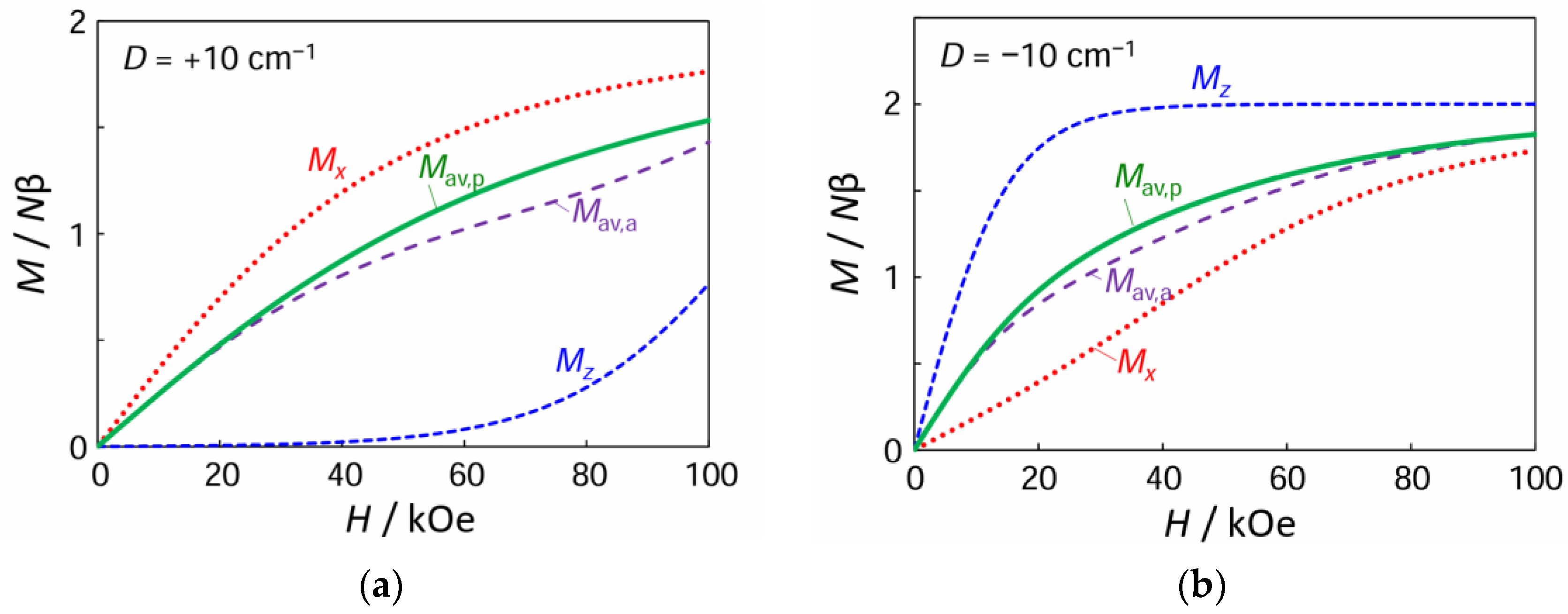
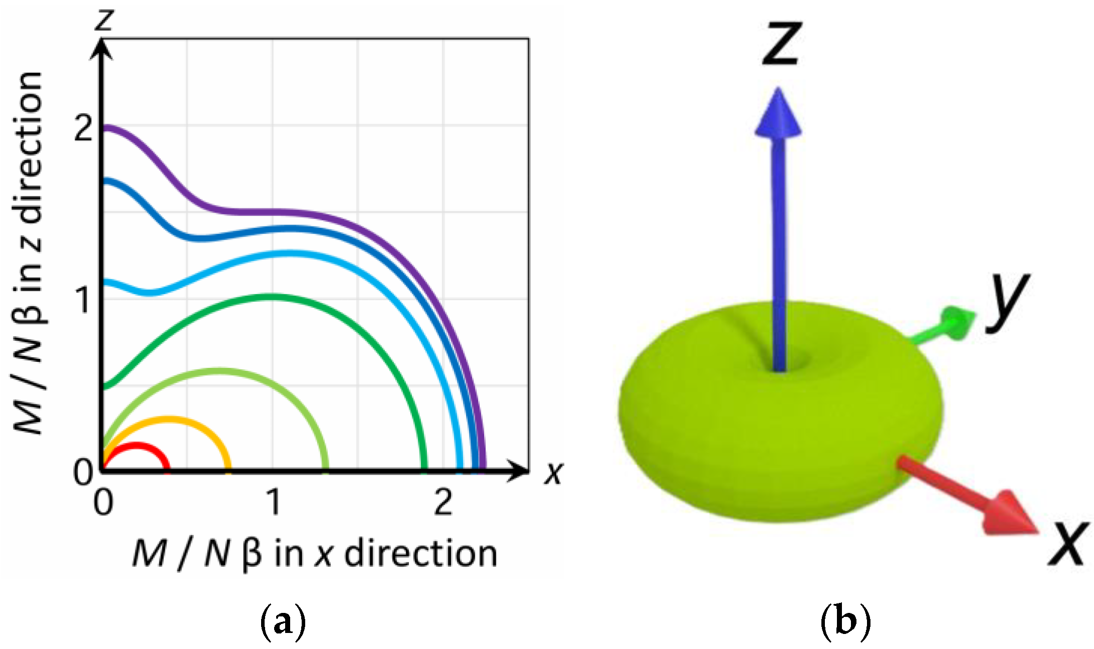
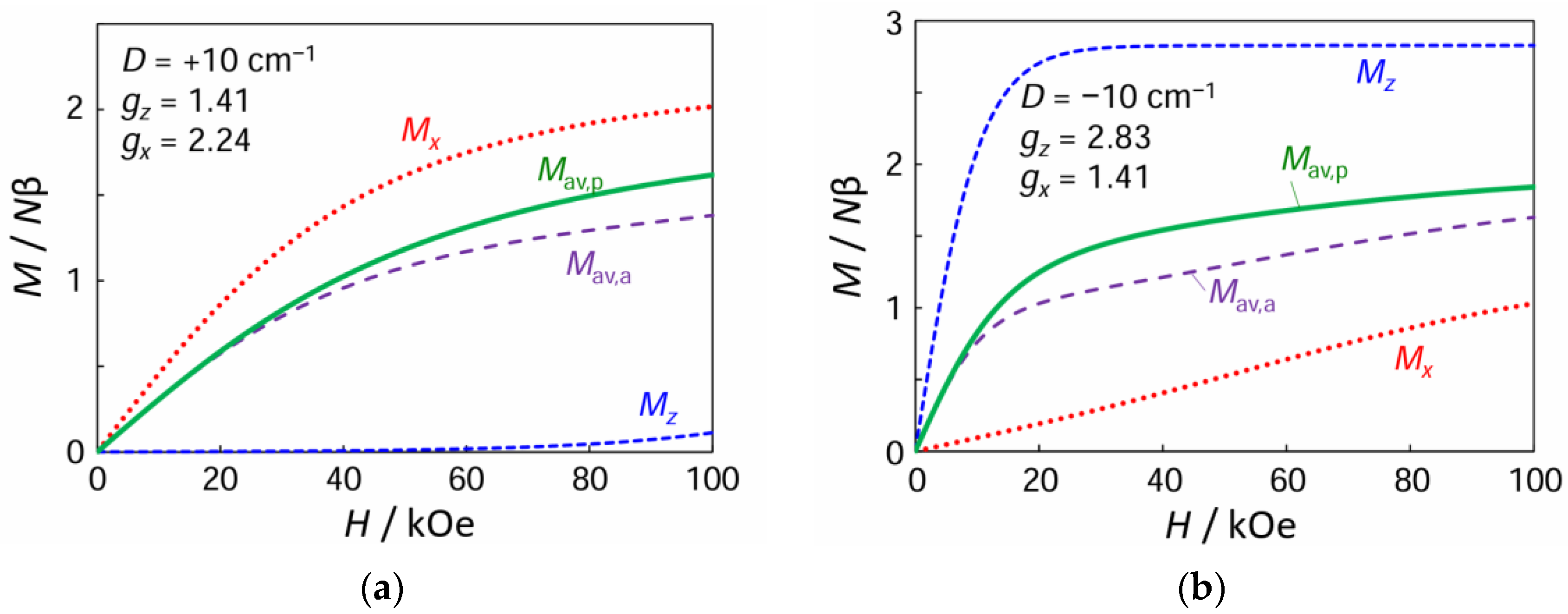
3.6. Powder Average Magnetization and Arithmetic Average Magnetization

For future reference, the present study compares the powder average magnetization M_av,p and the arithmetic average magnetization M_av,a for the S = 1 system. The theoretical magnetization curves are drawn in Figure 9 and Figure 10, using the equations in Appendix B and Appendix C and Equation (4). In both cases in Figure 9, g_z = g_x = 2.00 is assumed in axial symmetry, and M_z and M_x are drawn together. In Figure 9a, D is assumed to be +10 cm⁻¹, and in Figure 9b, D is assumed to be −10 cm⁻¹. (Please note that at D = 0 cm⁻¹, M_z, M_x, M_av,a, and M_av,p are all equal to the Brillouin function). In both Figure 9a,b, each M_av,a curve is close to each M_av,p curve in the low field region. This is concordant with the fact that the arithmetic average magnetic susceptibility is equal to the powder average as long as the magnetic field is weak enough to maintain additivity.

The significant g-anisotropy cases are simulated, as shown in Figure 10. In the weak magnetic field region, the arithmetic average magnetization is equal to the powder average, as in the g-isotropic case. The difference from the g-isotropic cases is the behavior in the high-field region where the magnetization approaches saturation, i.e., the difference between the arithmetic average and the powder average is larger at high magnetic fields when the g-anisotropy is large. The effect of the g-factor on the magnetization curves can be understood by the additivity of the square of the g-value. In terms of the g-value, the g-value is not additive, but the square of the g-value is additive. The slope of magnetization (magnetic susceptibility) in a weak magnetic field, where magnetization is proportional to the magnetic field, is proportional to the square of the g-value, and is additive, meaning that the arithmetic average and the powder average are equal. However, since saturation magnetization is proportional to the g-value, it is no longer additive, and the arithmetic average is not a good approximation for a strong magnetic field. It is important to consider g-anisotropy in the simulation because it affects the powder average, especially at high magnetic fields.

4. Conclusions

In this study, octahedral nickel(II) complexes were prepared with (omp)⁻ ligand. Complex 1 was characterized as a bulk sample, and its powder electronic spectra were analyzed based on the AOM calculation, which concluded that the spectra were typical of D₄-symmetric octahedral coordination geometry with a weak axial ligand field. Crystal structures were determined for 2 and 3, and the DFT computations based on the crystal structures indicated that the octahedral coordination geometry around the nickel(II) ions in 2 and 3 are both approximated as the D₄ rotation group and the weak axial ligand field (e_z < e_x,y) was suggested. The D₄ symmetry and the axially weak ligand field around the central nickel(II) ion may be due to the nature of the (omp)⁻ ligand and the complex cation structure in 1 is considered to be the same as that in 2. The temperature dependence of magnetic susceptibility and field dependence of magnetization were measured for 1, and the obtained data were simultaneously analyzed, considering the axial g-factors (g_z and g_x), the axial zero-field splitting (D), temperature-independent paramagnetism (χ_tip), and intermolecular interaction (zJ). The complex exhibited positive D value and the g_z < g_x relationship, which are both consistent with the weak axial ligand field (e_z < e_x,y) found by the electronic spectra for 1 and also by the DFT computations based on the crystal structure of 2.

This study also derived exact algebraic expressions for magnetization in the axial symmetry for the S = 1 system (Appendix C), and the magnetic anisotropy was expressed as the orientation-dependent magnetization caused by the zero-field splitting (D) and g-anisotropy. In addition, the importance of g-anisotropy in magnetization fitting was also demonstrated.

References

1. Figgis, B.N.; Hitchman, M.A. Ligand Field Theory and Its Application; Wiley-VCH: New York, NY, USA, 2000. [Google Scholar]
2. Boča, R. Zero-field splitting in metal complexes. Coord. Chem. Rev. 2004, 248, 757–815. [Google Scholar] [CrossRef]
3. Krzystek, J.; Ozarowski, A.; Telser, J. Multi-frequency, high-field EPR as a powerful tool to accurately determine zero-field splitting in high-spin transition metal coordination complexes. Coord. Chem. Rev. 2006, 250, 2308–2324. [Google Scholar] [CrossRef]
4. Kahn, O. Molecular Magnetism; VCH Publishers, Inc.: New York, NY, USA, 1993; pp. 17–21. [Google Scholar]
5. Sakiyama, H.; Chiba, Y.; Tone, K.; Yamasaki, M.; Mikuriya, M.; Krzystek, J.; Ozarowski, A. Magnetic Properties of a Dinuclear Nickel(II) Complex with 2,6-Bis[(2-hydroxyethyl)methylaminomethyl]-4-methylphenolate. Inorg. Chem. 2017, 56, 138–146. [Google Scholar] [CrossRef] [PubMed]
6. Gómez-Coca, S.; Aravena, D.; Morales, R.; Ruiz, E.J. Large magnetic anisotropy in mononuclear metal complexes. Coord. Chem. Rev. 2015, 289–290, 379–392. [Google Scholar] [CrossRef]
7. Zabala-Lekuona, A.; Seco, J.M.; Colacio, E. Single-Molecule Magnets: From Mn12-ac to dysprosium metallocenes, a travel in time. Coord. Chem. Rev. 2021, 441, 213984. [Google Scholar] [CrossRef]
8. Caneschi, A.; Gatteschi, D.; Sessoli, R.; Barra, A.L.; Brunel, L.C.; Guillot, M. Alternating current susceptibility, high field magnetization, and millimeter band EPR evidence for a ground S = 10 state in [Mn12O12(CH3COO)16(H2O)4]∙2CH3COOH∙4H2O. J. Am. Chem. Soc. 1991, 113, 5873–5874. [Google Scholar] [CrossRef]
9. Sessoli, R.; Tsai, H.-L.; Schake, A.R.; Wang, S.; Vincent, J.B.; Folting, K.; Gatteschi, D.; Christou, G.; Hendrickson, D.N. High-Spin Molecules: [Mn12O12(O2CR)16(H2O)4]. J. Am. Chem. Soc. 1993, 115, 1804–1816. [Google Scholar] [CrossRef]
10. Boča, R.; Rajnák, C. Unexpected behavior of single ion magnets. Coord. Chem. Rev. 2021, 430, 213657. [Google Scholar] [CrossRef]
11. Sakiyama, H.; Yamamoto, Y.; Hoshikawa, R.; Mitsuhashi, R. Crystal Structures and Magnetic Properties of Diaquatetrapyridinenickel(II) and Diaquatetrapyridinecobalt(II) Complexes. Magnetochemistry 2023, 9, 14. [Google Scholar] [CrossRef]
12. Sanyal, R.; Kundu, P.; Rychagova, E.; Zhigulin, G.; Ketkov, S.; Ghosh, B.; Chattopadhyay, S.K.; Zangrando, E.; Das, D. Catecholase activity of Mannich-based dinuclear CuII complexes with theoretical modeling: New insight into the solvent role in the catalytic cycle. New J. Chem. 2016, 40, 6623–6635. [Google Scholar] [CrossRef]
13. Sakiyama, H.; Mochizuki, R.; Sugawara, A.; Sakamoto, M.; Nishida, Y.; Yamasaki, M. Dinuclear zinc(II) complex of a new acyclic phenol-based dinucleating ligand with four methoxyethyl chelating arms: First dizinc model with aminopeptidase function. J. Chem. Soc. Dalton Trans. 1999, 997–1000. [Google Scholar] [CrossRef]
14. Sakiyama, H.; Igarashi, Y.; Nakayama, Y.; Hossain, M.d.J.; Unoura, K.; Nishida, Y. Aminopeptidase function of dinuclear zinc(II) complexes of phenol-based dinucleating ligands: Effect of p-substituents. Inorg. Chim. Acta 2003, 351, 256–260. [Google Scholar] [CrossRef]
15. Bain, G.A.; Berry, J.F. Diamagnetic corrections and Pascal’s constants. J. Chem. Educ. 2008, 85, 532. [Google Scholar] [CrossRef]
16. Hoshikawa, R.; Mitsuhashi, R.; Asato, E.; Liu, J.; Sakiyama, H. Structures of dimer-of-dimers type defect cubane tetranuclear copper(II) complexes with novel dinucleating ligands. Molecules 2022, 27, 576. [Google Scholar] [CrossRef] [PubMed]
17. Sheldrick, G.M. A short history of SHELX. Acta Cryst. Sect. A 2008, 64, 112–122. [Google Scholar] [CrossRef] [PubMed]
18. Sheldrick, G.M. Crystal structure refinement with SHELXL. Acta Cryst. Sect. C 2015, 71, 3–8. [Google Scholar] [CrossRef] [PubMed]
19. Schmidt, M.W.; Baldridge, K.K.; Boatz, J.A.; Elbert, S.T.; Gordon, M.S.; Jensen, J.H.; Koseki, S.; Matsunaga, N.; Nguyen, K.A.; Su, S.; et al. General atomic and molecular electronic structure system. J. Comput. Chem. 1993, 14, 1347–1363. [Google Scholar] [CrossRef]
20. Gordon, M.S.; Schmidt, M.W. Advances in Electronic Structure Theory; Elsevier: Amsterdam, The Netherlands, 2005. [Google Scholar]
21. Tawada, Y.; Tsuneda, T.; Yanagisawa, S.; Yanai, T.; Hirao, K. A long-range-corrected time-dependent density functional theory. J. Chem. Phys. 2004, 120, 8425–8433. [Google Scholar] [CrossRef] [PubMed]
22. Sakiyama, H. Development of MagSaki software for magnetic analysis of dinuclear high-spin cobalt(II) complexes in an axially distorted octahedral field. J. Chem. Software 2001, 7, 171–178. [Google Scholar] [CrossRef]
23. Sakiyama, H. Development of MagSaki(A) software for the magnetic analysis of dinuclear high-spin cobalt(II) complexes considering anisotropy in exchange interaction. J. Comput. Chem. Jpn. 2007, 6, 123–134. [Google Scholar] [CrossRef]
24. Sakiyama, H. Development of MagSaki(Tri) software for the magnetic analysis of trinuclear high-spin cobalt(II) complexes. J. Comput. Chem. Jpn. Int. Ed. 2015, 1, 9–13. [Google Scholar] [CrossRef]
25. Sakiyama, H. Development of MagSaki(Tetra) software for the magnetic analysis of tetranuclear high-spin cobalt(II) complexes. J. Comput. Chem. Jpn. Int. Ed. 2016, 2, 2016-0001. [Google Scholar] [CrossRef]
26. Sakiyama, H.; Sudo, R.; Abiko, T.; Yoshioka, D.; Mitsuhashi, R.; Omote, M.; Mikuriya, M.; Yoshitake, M.; Koikawa, M. Magneto-structural correlation of hexakis-dmso cobalt(II) complex. Dalton Trans. 2017, 46, 16306. [Google Scholar] [CrossRef] [PubMed]
27. Sakiyama, H.; Abiko, T.; Ito, M.; Mitsuhashi, R.; Mikuriya, M.; Waki, K.; Usuki, T. Reversible crystal-to-crystal phase transition of an octahedral zinc(II) complex with six dimethylsulfoxide. Polyhedron 2019, 158, 494–498. [Google Scholar] [CrossRef]
28. Sakiyama, H.; Suzuki, T.; Ono, K.; Ito, R.; Watanabe, Y.; Yamasaki, M.; Mikuriya, M. Synthesis, structure, and magnetic properties of dinuclear nickel(II) complexes with a phenol-based dinucleating ligand with four methoxyethyl chelating arms. Inorg. Chim. Acta 2005, 358, 1897–1903. [Google Scholar] [CrossRef]
29. Yamaguchi, R.; Tasaki, M.; Asato, E.; Sakiyama, H. Synthesis and Crystal Structure of a Nickel(II) Complex with Bis(2-methoxyethyl)amine. X-ray Struct. Anal. Online 2011, 27, 5–6. [Google Scholar] [CrossRef]
30. Bendix, J.; Schäffer, C.E.; Brorson, M. Quantitative formulation of ligand field theory by the use of orthonormal operators. Exemplification by means of pq systems. Coord. Chem. Rev. 1989, 94, 181–241. [Google Scholar] [CrossRef]
31. Kudrat-E-Zahan, M.; Nishida, Y.; Sakiyama, H. Identification of cis/trans isomers of bis(acetylacetonato)nickel(II) complexes in solution based on electronic spectra. Inorg. Chim. Acta 2010, 363, 168–172. [Google Scholar] [CrossRef]
32. Mabbs, F.E.; Machin, D.J. Magnetism and Transition Metal Complexes; Dover Publications, Inc.: Mineola, NY, USA, 2008. [Google Scholar]
33. Griffith, J.S. The Theory of Transition-Metal Ions; Cambridge University Press: Cambridge, UK, 1961. [Google Scholar]
34. Sakiyama, H.; Abiko, T.; Yoshida, K.; Shomura, K.; Mitsuhashi, R.; Koyama, Y.; Mikuriya, M.; Koikawa, M.; Mitsumi, M. Detailed magnetic analysis and successful deep-neural-network-based conformational prediction for [VO(dmso)5][BPh4]2. RSC Adv. 2020, 10, 9678–9685. [Google Scholar] [CrossRef]
Figure 1. Chemical structure of (onp).
Magnetochemistry 10 00032 g001
Figure 2. Crystal structure of [Ni(onp)(dmso)(H2O)]+ complex cation in 2. Hydrogen atoms are omitted for clarity. Thermal ellipsoids are drawn at the 50% probability level.
Magnetochemistry 10 00032 g002
Figure 3. Crystal structure of [Ni(onp)(dmf)2]+ complex cation in 3. Hydrogen atoms are omitted for clarity. Thermal ellipsoids are drawn at the 50% probability level.
Magnetochemistry 10 00032 g003
Figure 4. The energy levels of d-orbital-related molecular orbitals for [Ni(onp)(dmso)(H2O)]+ complex cation in 2 based on the DFT computation (LC-BOP/6-31G**).
Magnetochemistry 10 00032 g004
Figure 5. The energy levels of d-orbital-related molecular orbitals for [Ni(onp)(dmf)2]+ complex cation in 3 based on the DFT computation (LC-BOP/6-31G**).
Magnetochemistry 10 00032 g005
Figure 6. Powder electronic spectra and energy levels of 1: (a) observed spectra (), spectral components (·····), and sum of the components (---); (b) energy levels of the states in the D4 symmetry obtained from the spectral analysis.
Magnetochemistry 10 00032 g006
Figure 7. The χAT versus T plot and M versus H plot (insertion) for 1. The observed data () and the theoretical curves () with the best-fitting parameter set (gz, gx, D, zJ, χtip) = (2.13, 2.31, +5.9 cm−1, −0.70 cm−1, 534 × 10−6 cm3 mol−1).
Magnetochemistry 10 00032 g007
Figure 8. Magnetic anisotropy at 2 K with the parameter set (gz, gx, D, zJ, χtip) = (2.13, 2.31, +5.9 cm−1, −0.70 cm−1, 534 × 10−6 cm3 mol−1): (a) cross-sectional view of the spatial distribution of magnetization in the xz plane at 5 kOe (red), 10 kOe (orange), 20 kOe (yellow-green), 40 kOe (green), 60 kOe (light blue), 80 kOe (blue), and 100 kOe (violet); (b) three-dimensional representation of magnetization at 5 kOe.
Magnetochemistry 10 00032 g008
Figure 9. Comparison of powder average magnetization (Mav,p) and arithmetic average magnetization (Mav,a) in the g-isotropic cases (g = 2.00) at 2 K. Mz and Mx curves are also drawn: (a) when D = +10 cm−1; (b) when D = −10 cm−1.
Magnetochemistry 10 00032 g009
Figure 10. Comparison of powder average magnetization (Mav,p) and arithmetic average magnetization (Mav,a) when g-anisotropy is significant at 2 K. Mz and Mx curves are also drawn: (a) when D = +10 cm−1, gz = 1.41, and gx = 2.24; (b) when D = −10 cm−1, gz = 2.83, and gx = 1.41.
Magnetochemistry 10 00032 g010