Numerical Study of Lateral Migration of Elliptical Magnetic Microparticles in Microchannels in Uniform Magnetic Fields


Department of Mechanical and Aerospace Engineering, Missouri University of Science and Technology, 400 W. 13th St., Rolla, MO 65409, USA
*
Author to whom correspondence should be addressed.
Magnetochemistry 2018, 4(1), 16; https://doi.org/10.3390/magnetochemistry4010016
Submission received: 18 December 2017
/
Revised: 10 January 2018
/
Accepted: 29 January 2018
/
Published: 12 February 2018
(This article belongs to the Special Issue Magnetic Fields in Microfluidic Systems)
Abstract
:This work reports numerical investigation of lateral migration of a paramagnetic microparticle of an elliptic shape in a plane Poiseuille flow of a Newtonian fluid under a uniform magnetic field by direct numerical simulation (DNS). A finite element method (FEM) based on the arbitrary Lagrangian–Eulerian (ALE) approach is used to study the effects of strength and direction of the magnetic field, particle–wall separation distance and particle shape on the lateral migration. The particle is shown to exhibit negligible lateral migration in the absence of a magnetic field. When the magnetic field is applied, the particle migrates laterally. The migration direction depends on the direction of the external magnetic field, which controls the symmetry property of the particle rotational velocity. The magnitude of net lateral migration velocity over a cycle is increased with the magnetic field strength when the particle is able to execute complete rotations, expect for = 45° and 135°. By investigating a wide range of parameters, our direct numerical simulations yield a comprehensive understanding of the particle migration mechanism. Based on the numerical data, an empirical scaling relationship is proposed to relate the lateral migration distance to the asymmetry of the rotational velocity and lateral oscillation amplitude. The scaling relationship provides useful guidelines on design of devices to manipulate nonspherical micro-particles, which have important applications in lab-on-a-chip technology, biology and biomedical engineering.
1. Introduction
For decades, magnetic fields have been widely used to separate microscale and nanoscale magnetic particles suspended in fluids in various industrial, biological and biomedical applications, such as mineral purification [1], cell separation [2], and targeted drug delivery [3]. The underlying principle in these applications is magnetophoresis—the motion of particles due to magnetic forces. The generation of magnetic forces requires both a magnetic particle and a spatially non-uniform magnetic field (or non-zero magnetic field gradients) [4].
Recent experiments have demonstrated a non-conventional strategy to manipulate magnetic particles by combining a magnetic torque, non-spherical shapes and shear flows [5,6]. Different from traditional techniques based on forces, this torque-based method only requires a uniform magnetic field. As a result, there is no magnetic force, and thus, the method may be better described as “force-free magnetophoresis”. Here, the lateral migration of non-spherical particles stems from the coupling of the magnetic field, flow field and particle–wall hydrodynamic interactions. While earlier experiments provide the first observations of this unique phenomenon, it remains difficult to conduct well-controlled experimental studies. On the other hand, numerical simulations are powerful tools to carry out systematic investigations to gain insights on various factors that influence the particle transport behaviours.
Due to its importance to science and engineering, the dynamics of non-spherical particles in flows have been a subject of extensive theoretical, numerical and experimental investigations. For example, the pioneering work includes Jeffery’s theory [7] and experimental studies by Mason’s group [8,9]. With the advancement of computing capabilities, numerical simulations have been increasingly employed to study the motion of both spherical and non-spherical particles in a variety of shear flows, including plane Couette and Poiseuille flows. Feng et al. [10] reported a direction numerical simulation (DNS) based on the finite element method (FEM) to study the lateral migration of the neutrally and non-neutrally buoyant circular particle in plane Couette and Poiseuille flows. The simulation results agree qualitatively with the results of perturbation theories and experimental data. Gavze and Shapiro [11] used a boundary integral equation method to investigate the effect of particle shape on forces and velocities acting on the particle near the wall in a shear flow. Pan’s group proposed a distributed Lagrange-multiplier-based fictitious domain method (DLM) to investigate the motion of multiple neutrally buoyant circular cylinders and elliptical cylinders in shear flow [12,13] and plane Poiseuille flow [14,15]. Yang et al. [16] reported two methods, the arbitrary Lagrangian–Eulerian (ALE) method and the distributed Lagrange-multiplier-based fictitious domain method (DLM), to study the migration of a single neutrally buoyant rigid sphere in tube Poiseuille flow. Ai et al. [17] investigated some key factors on pressure-driven transport of particles in a symmetric converging-diverging microchannel by the ALE finite-element method. Lee et al. [18,19] used the same method as Gavze and Shapiro [11] to study the particle transport behaviour with different size, shape and material properties in the plane Couette flow.
Motions of magnetic particles have been numerically investigated due to their close relevance to biomedical separations [20] and magnetically assisted drug delivery [21]. Smistrup et al. [22] used numerical simulations to study magnetic separation of magnetic beads in the microchannel under the magnetic field of microfabricated electro-magnets. Their simulation results agree qualitatively with the experimental data. Sinha et al. [23] numerically investigated the motion of magnetic microbeads in the microchannel under a non-uniform magnetic field. More recently, shape-dependent drag force and magnetization have been exploited to separate non-magnetic particles and biological cells in a ferrofluid [24,25]. In prior works, the particles are often treated as point masses while the effect of hydrodynamic interactions resulting from particle shape and finite size are not directly considered.
Our previous work focused experimentally on lateral migration when the particle is undergoing rotational motion [5,6]. The work by Matsunaga et al. mainly discussed lateral migration, which occurred when particles are not rotating [26,27]. The work by Cao et al. numerically studied the rotation and lateral migration of particles for both scenarios including weak and strong field strengths [28]. The present work studies the effects of strength and direction of the magnetic field strength, initial particle position, particle aspect ratio, and particularly proposes a scaling relationship between the symmetry properties of the particle’s rotational velocity, and the magnitude of lateral oscillation in the absence of a magnetic field. By implementing an ALE method in the COMSOL FEM solver, our direct numerical simulations couple and simultaneously solve the flow field, magnetic field, and particle motions. The magnetic torque, hydrodynamic torque as well as hydrodynamic force are computed and used to determine the translational and rotational motions of the particle via Newton’s second law and Euler’s law. After validating the numerical model with Jeffery’s theory, systematic numerical simulations are carried out to understand the roles of key factors, including the strength and direction of the magnetic field, particle aspect ratio, and initial particle–wall separation distance, on the lateral migration of the particle.
2. Simulation Method
2.1. Mathematical Model
We consider a prolate elliptical particle immersed in a plane Poiseuille flow of an incompressible Newtonian fluid with density and dynamic viscosity as shown in Figure 1. The computational domain, , is surrounded by the boundary, ABCD, and particle surface, . The width and length of the computational domain are W and L, respectively. The particle aspect ratio is , where a and b are the major and minor semi-axis lengths of the particle, respectively. The particle–wall separation distance, , is defined as the vertical distance between the particle center and the x-axis. The orientation of the particle, , is defined as the angle between the major axis of the particle and positive y-axis. A uniform magnetic field, , is imposed at an arbitrary direction, denoted by , as shown in Figure 1.
The flow field, u, is governed by the continuity equation and Navier-Stokes (NS) equations for an incompressible and Newtonian flow:
where p is the pressure and t is the time.
To obtain a fully developed laminar flow profile, the laminar inflow is at the inlet AC. The zero normal pressure condition is set to the outlet BD. No-slip condition is applied on channel walls AB and CD. No-slip condition also applies on the particle surface, so the fluid velocities on the particle surface are given as:
where and are translational and rotational velocities of particle, respectively. and are the position vectors of the surface and the center of the particle. The hydrodynamic force and torque acting on the particle are expressed as:
where is the hydrodynamic stress tensor.
The governing equations of the magnetic field are given as:
where H and B are the magnetic field strength and the magnetic flux density, respectively. To obtain a uniform magnetic field, the magnetic scalar potential difference is set to AB and CD. A zero magnetic potential = 0 is set to AB and a magnetic potential = is set to CD. The magnetic insulation condition is set at AC and BD. Since the magnetic field is uniform and the particle is paramagnetic, the force acting on the particle is zero. Assuming the magnetic particle is homogeneous, isotropic, and linearly magnetizable, the magnetic torque acting on particle is expressed as [29]:
where and are the magnetic fields inside and outside the particle, respectively, is the magnetic susceptibility of the particle, is the magnetic permeability of the vacuum, and is the volume of particle.
The translation and rotation of the particle are governed by Newton’s second law and Euler’s equation:
where and are the mass and the moment of inertia of the particle. Since the particle rotation is in the plane, only the z-component of , and are necessary to calculate the rotational velocity, and .
The position of center and orientation of particle are given by:
where and are the initial position and orientation of the particle.
The position and orientation of the particle will affect the magnetic and flow fields around the particle, and successively alter the magnetic torque and hydrodynamic force and torque acting on the particle. Therefore, we use direct numerical simulation (DNS) based on the finite element method (FEM) and arbitrary Lagrangian–Eulerian (ALE) method to account for such coupling among the particle, fluid flow, and magnetic fields. A similar method has been successfully achieved by Hu et al. [30] and Ai et al. [17,31,32,33]. Numerical models are implemented by using a commercial FEM solver COMSOL Multiphysics. First, we use the stationary solver for parametric sweep analysis to simulate the magnetic field inside and outside of the particle, and calculate the magnetic torque acting on the particle. Then, a two-way coupling fluid–particle interaction model is solved by using a time-dependent solver, where the magnetic torque is imported into the model as a variable. Quadratic triangular elements are generated in the simulations. Fine mesh around the particle and finer mesh around the tip of the particle are created to accurately calculate the hydrodynamic force and torque acting on the particle.
2.2. Material Properties Used in Simulations
In this study, the fluid and particles in the simulations are water and magnetite-doped polystyrene particle, respectively. The density and dynamic viscosity of water are 1000 kg/m3 and Pa·s, respectively. The magnetic susceptibility of particle is according to previous studies [5,6], whereas the fluid is a non-magnetic fluid. The density of the particle is 1100 kg/m3. The particles used in the simulation have varying aspect ratios, but all have the same volume, which is equal to the volume of a 7 µm-diameter circular particle. The width and length of the computational domain are W = 800 µm and L = 50 µm, respectively. Inlet flow velocity is 2.5 mm/s, so Re = 0.125.
2.3. Grid Independence Analysis
Grid independence analysis is presented to determine the appropriate meshes for a fast and accurate numerical simulation. The results of six different meshes in a plane Poiseuille flow in the absence of the magnetic field are shown in Table 1 and Figure 2. As can be seen, the numerical results are good enough when the domain element number is larger than 11,600 and the boundary element number on the particle surface is larger than 120. Thus, in the paper, we used about 12,000 elements in the computational domain in Figure 1, and about 150 elements on the particle surface , which could give reasonably accurate results.
3. Results and Discussion
3.1. Validation of Numerical Method
To validate our numerical method, we first compare the results of our simulation to Jeffery’s theory, which describes the periodic rotation of an axisymmetric ellipsoidal particle in a simple shear flow [7]. The period of the particle rotating from to is , where is the shear rate. Due to the fore-aft symmetry of the particle, here we define as the period of rotation from 0 to , i.e., . Figure 3 shows the particle rotation predicted by Jeffery’s theory and our simulation for a particle having in a simple shear flow with shear rate = 200 in the absence of a magnetic field. The theoretical value of from the Jeffery theory is 0.0668 s, while the period obtained in our FEM simulation is 0.0670 s. The relative error is 0.37%, suggesting that the simulation has a remarkable agreement with the theory. Therefore, this simulation method has been validated to be sufficiently accurate to study the periodic rotation of particle in this work.
3.2. Particle Motion without a Magnetic Field
In this section, we investigate the effect of particle aspect ratio, , and its initial particle–wall separation distance, , on particle motion without a magnetic field. Figure 4 shows the trajectory of an elliptical particle with initially located at µm. As can be seen, the particle oscillates away from the wall in the first half period (from to ) and towards the wall in the second half period (from to ), but there is a negligible net lateral migration. We define the difference between the maximum and minimum values of the oscillatory motion in the y-direction as the amplitude, A, as shown in Figure 4a, and define the period as the time spent by the particle to rotate from to , , as shown in Figure 4b.
The orientation of the particle, , as a function of the dimensionless time, , over a period is shown in Figure 4c. As can be seen, the particle has a symmetry of rotation with respect to . The rotational velocity due to the shear flow is symmetric about as shown in Figure 4d, meaning that the particle spends the same amount of time in the first and second half periods. The presence of the wall induces particle–wall hydrodynamic interaction, which causes the oscillatory motion of the elliptical particle. However, due to the equal time the particle spends in the first and second half rotational period, the lateral distance of the particle moving upwards and moving downwards are equal. Thus, there is no net lateral migration.
The lateral migration of the elliptical particle for three initial particle–wall separation distances , and different aspect ratio , are shown in Figure 5a,b. In Figure 5a, as is increased from 12 µm to 16 µm, the period of rotation becomes longer, and the amplitude A becomes smaller for a fixed . As is decreased from 4 to 2, the period of rotation becomes shorter, and the amplitude A becomes smaller for a fixed (Figure 5b). For example, at µm, the period of rotation = 0.1295 s and the amplitude A = 0.6547 µm for ; = 0.0844 s and A = 0.3137 µm for = 3; = 0.0556 s and A = 0.0841 µm for = 2. Furthermore, the net lateral migration is almost zero, regardless of its initial particle–wall separation distance and aspect ratio. It is consistent with our previous experimental observation [6].
The amplitude and period of the oscillatory motion for different and different are shown in Figure 5c,d. As can be seen, for a fixed , the curve becomes steeper when the particle approaches the wall (i.e., is decreased). The slope of the curve becomes larger when the particle shape becomes more non-spherical ( is increased). Figure 5d shows the dimensionless period of rotation, , varying with the dimensionless particle–wall separation distance, , is the period of Jeffery’s orbit calculated by using the shear rate at the position of the particle centroid and a is the semi-major axis of the particle, respectively. As can be seen in Figure 5d, the dimensionless time, , is larger than 1 for the all results. As is increased, is decreased first and then is increased for a constant . Furthermore, the decreasing rate in the first part and the increasing rate in the second part of become steeper as AR increases from 2 to 4.
The effect of and on A and in Figure 5c,d can be explained as follows. When the particle is transported in the channel flow, the wall induces particle–wall hydrodynamic interactions and increases resistance on the rotation of particle [11,34]. The smaller the particle–wall separation ( varying from 16 µm to 12 µm) is, the more prominent the particle–wall interaction is. The amplitude (A) thus increases with decreasing i.e., increased hydrodynamic interactions, as shown in Figure 5c). On the other hand, the particle aspect ratio represents the degree of deviation from the spherical particle. A larger particle aspect ratio induces more prominent particle–wall interaction than a spherical particle (). The increasing resistance on the rotation of particle causes the particle spending longer time than that in the absence of the wall. Therefore, the particle–wall separation distance and particle aspect ratio are two important factors affecting the oscillatory motion of the particle in the microchannel.
3.3. Particle Motion in a Magnetic Field
3.3.1. Magnetic Field at
In this section, we investigate the effect of magnetic fields with the direction on the lateral migration of the particle. The particle with is initially placed at = 12 µm. The magnetic field of A/m is imposed at the direction of . Figure 6a,b shows the particle orientation angle and the lateral migration as a function of time. For convenience of discussion, we define a dimensionless parameter, , as the ratio of the time that the particle rotates from to to the entire period of the particle rotation as shown in Figure 6a. Here, the period of particle rotation is defined the same as in Section 3.2. To distinguish the period of rotation from Section 3.2, we use T as the period of rotation when the magnetic field is applied. As can be seen in Figure 6a, when , and the curve is anti-symmetric to ; when the magnetic field strength A/m, and the curve is no longer anti-symmetric to . Thus, we can use the dimensionless parameter to characterize the symmetry and asymmetry property of the particle’s rotation. Second, we define the net lateral migration of the particle, , as the difference between the position of particle centroid at and at in the y-direction as shown in Figure 6b. As can be seen, when a magnetic field is applied at , , meaning that the particle moves away from the channel wall over a period.
The influence of the perpendicular magnetic field can be explained as follows. In the absence of a magnetic field, the hydrodynamic torque causes the rotational motion of the particle. The corresponding rotational velocity is shown as the dashed line in Figure 6c. As we discussed before, there is a negligible net migration due to the symmetry of the particle rotational velocity. When a magnetic field is applied at , the total rotational velocity, , is asymmetric with respect to , shown as the solid line in Figure 6c. The rotational velocity due to the magnetic field, , and the rotational velocity due to the hydrodynamic torque, have opposite directions when the particle orientation is between to ; and have the same direction when . As a result, the particle spends more time in the first half period than in the second half period, causing the asymmetry of the particle rotational velocity. The asymmetric particle rotation further leads to a broken symmetry of the particle’s lateral oscillation motion, via hydrodynamic interactions [11]. Consequently, the particle spends more time moving upwards than moving downwards, and exhibits a net lateral migration away from the wall, as shown in Figure 6b.
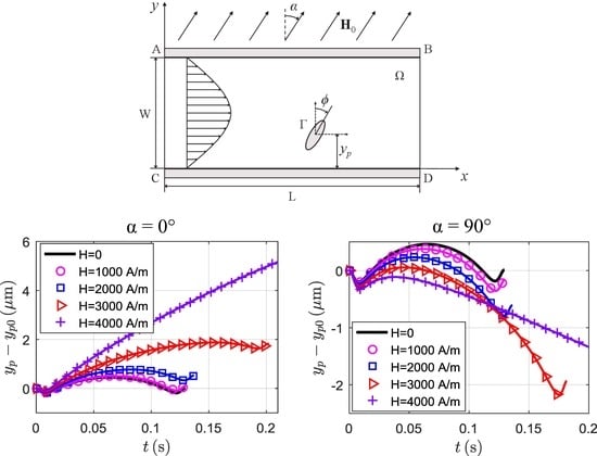
We investigate the effect of the magnetic field strength on the particle rotation and lateral migration. Figure 7a shows the orientation of the particle, , with time, t, in one period for different magnetic field strengths. As can be seen, when the magnetic field is applied, the period of rotation becomes longer as compared to that without a magnetic field (). From Figure 7a, we can see that the period of rotation, T, is increased as the magnetic field strength is increased from = 1000 A/m to 3000 A/m. In this case, there are two factors affecting the period of rotation. One is the magnetic field. In the simple shear flow, as the magnetic field strength is increased, the period of rotation is increased when = 0° [35]. The other factor is the decreased shear rate as the particle moved toward the center. The magnetic field caused the particle to migrate towards the center, where the shear rate is decreased. Thus, the magnetic field coupled with the nonlinear shear rate induced the increase of period of the rotation. Figure 7b shows the dependence of dimensionless parameter, , on the magnetic field strength. When the magnetic field strength is applied, , meaning that the symmetry of particle rotation is broken. As the magnetic field strength increases, increases, meaning that the asymmetry of the particle rotation becomes more pronounced. This asymmetry of particle rotation, combined with oscillatory motion, causes the net lateral migration. Figure 7c shows the net migration of particle, , as a function of time, t, in one period for different magnetic field strengths. Because , the particle moves upwards, and the net lateral migration, , increases with the increase of the magnetic field strength.
To characterize the net lateral migration, we define an average vertical migration velocity, , which is the net lateral migration over the rotational period of the particle. The average vertical velocity, , for different magnetic field strengths are shown in Figure 7d. As can be seen, the vertical velocity increases when the magnetic field strength increases from 0 to 3000 A/m. This means that the particle moves upwards faster as the magnetic field increases. Furthermore, as can be seen in Figure 7a,d, when the magnetic field strength is 4000 A/m, the particle could not perform a complete rotation but continuously moved upwards. The reason for the impeded rotation is because of the dynamic balances between the hydrodynamic and magnetic torques. Due to the parabolic velocity profile of the Poiseuille flow, the shear rate becomes smaller closer to the channel center. As a result, the particle orientation continuously decreases as the particle moves towards the channel center.
3.3.2. Magnetic Field at
In this section, we investigate the effect of magnetic fields with the direction on the lateral migration of the elliptical particle. The particle with = 4 is initially located at = 12 µm. The magnetic field with a strength of 3000 A/m is imposed at the direction of . The orientation and the lateral migration varying with time are shown in Figure 8. When the magnetic field is applied at , and , as we can see in Figure 8a,b. The reason can be similarly explained for the case of . Here, the magnetic rotational velocity, , and the hydrodynamic rotational velocity, , have the same direction in the first half period and opposite directions in the second half period of rotation. The total rotational velocity, , is asymmetric with respect to , shown as the solid line in Figure 8c. The particle spends less time to move upwards in the first half period than the second half period. Therefore, the symmetry of the particle rotation is broken and there is a net lateral migration over one period.
For different magnetic field strength, as the magnetic field strength increases, the period of rotation becomes longer as shown in Figure 9a. It is the same as the case of . When the magnetic field strength is 4000 A/m, the particle could not perform a complete rotation as well. The difference between cases of and is the impeded orientation: the maximum orientation is larger than when , whereas the maximum orientation is smaller than when . Figure 9b shows the variation of with different magnetic field strengths. As we can see, and becomes smaller with an increase of the magnetic field strength, meaning the asymmetry of rotation becomes more pronounced. The lateral migration for different magnetic field strength, and the average vertical velocity, , are shown in Figure 9c,d, respectively. As the magnetic field strength is increased, the particle moves downwards quicker. Interestingly, when the magnetic field strength is 4000 A/m, the rate of the lateral migration becomes slower than H = 3000 A/m as shown in the line with plus symbol in Figure 9c.
3.3.3. Magnetic Field at
In this section, we investigate the effect of magnetic fields with on the lateral migration of the elliptical particle. When the magnetic field is imposed at , the total rotational velocity, , is symmetric to as shown in Figure 10a. For four different magnetic field strengths, the orientation varying with time is shown in Figure 10b. As the magnetic field strength is increased, the period of rotation becomes shorter, which is different from the results when the magnetic field is imposed at and 90°. However, the particle preserves the symmetry of rotational velocity as can be seen in Figure 10c: for these four magnetic field strengths. The lateral migration for different magnetic field strengths is shown in Figure 10d. The oscillatory amplitude is decreased with increasing the magnetic field strength, which is different from the results when the magnetic field is imposed at and 90°. Such a decrease of oscillation is due to the decrease of the rotational velocity, and translation-and-rotation coupling. There is no net migration as can be seen in Figure 10e. for these four magnetic field strengths that have been investigated.
3.3.4. Magnetic Field at
In this section, we investigate the effect of magnetic fields applied at on the lateral migration of the elliptical particle. When the magnetic field is imposed at , the total rotational velocity, , is symmetric to as shown in Figure 11a. When = 1000 A/m, and , meaning that the particle’s rotation velocity is symmetric about and there is no net lateral migration. However, when the magnetic field strength is equal or larger than 2000 A/m, the particle could not complete a full rotation, but continuously moves upwards as shown in Figure 11b,c. The lateral motion is due to the particle being pinned at a steady angle [26]. As the magnetic field strength is increased, the maximum orientation becomes smaller and the lateral migration becomes faster.
3.3.5. Effects of Particle Shape and the Wall
As we discussed in Section 3.2, the particle–wall separation distance and particle aspect ratio are two important factors on the oscillatory motion of the particle. In this section, we investigate the effect of these two factors on particle lateral migration with a magnetic field. Here, the magnetic field strength = 2000 A/m is applied at . The dimensionless parameter, , and the average vertical velocity, , for three different particle aspect ratios are shown in Figure 12(a1,a2). As the particle aspect ratio is increased, both and increase. The particle aspect ratio represents the degree of deviation from the spherical particle. As the particle shape deviates more from the spherical particle, the asymmetry of particle rotation becomes more pronounced, and the particle moves up faster. Therefore, particle aspect ratio is an essential factor on particle lateral migration when a magnetic field is applied. Figure 12(b1,b2) show the results when the particle is released at different initial particle–wall separation distances. is increased, but is decreased as is increased from 10 µm to 16 µm. As the particle is at a larger distance away from the wall, the asymmetry of particle rotation becomes more pronounced. However, the particle moves up slower, due to the small amplitude A.
3.4. Lateral Migration Mechanism
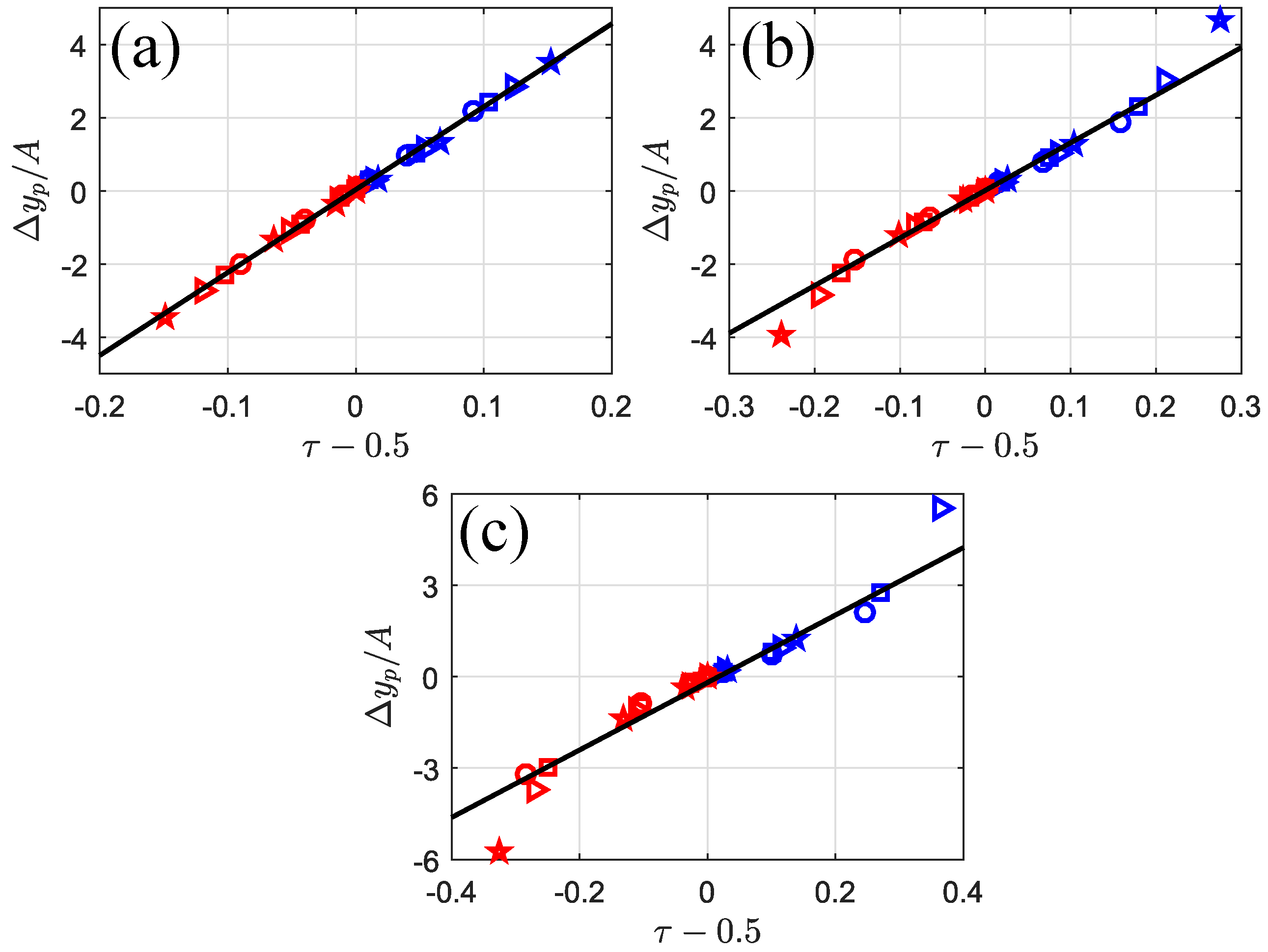
From previous analysis, we can see that the net lateral migration of the particle depends on the lateral oscillation and the asymmetric rotation. The particle lateral oscillation depends on the particle shape (aspect ratio ) and the proximity to the wall (initial particle–wall separation distance ). The larger deviation from the spherical shape and the closer to the wall are, the more pronounced particle–wall hydrodynamic interaction is [11]. The degree of particle–wall hydrodynamic interaction is characterized by the amplitude A for a fixed particle aspect ratio. The asymmetric rotation of the particle depends on the non-zero magnetic torque acting on the particle, which in turn depends on the field direction and magnitude. The direction of the magnetic field controls the nature of the asymmetry and thus the direction of the net lateral migration. When , the particle moves upwards; when , the particle move downwards. The strength of the magnetic field controls the speed of the lateral migration. The more deviates from 0.5, the larger the migration speed is. In other words, the direction of the magnetic field determines whether is positive or negative, and the strength of the magnetic field determines the absolute value of . Therefore, we use to characterize the asymmetric rotation of the particle. Based on the above analysis, we propose a scaling relationship, for all particle aspect ratios investigated, = 2, 3, 4. As shown in Figure 13, the numerical results and the linear fitted curves are shown as symbols and lines, respectively. The agreement between the fitted curves and numerical results confirms the scaling relationships. Our numerical results suggest that it is reasonably applicable when from Figure 13. However, due to the complex particle–wall hydrodynamic interactions, it is difficult to obtain a quantitative expression relating to A and . In this work, the linear scaling is fitted very well when , which can provide a useful guideline on the effective design for other researchers.
4. Conclusions
In this paper, we developed a multi-physics numerical model based on direct numerical simulations to investigate the lateral migration of a paramagnetic elliptical particle in a plane Poiseuille flow under a uniform magnetic field. When the magnetic field is absent, there is a negligible net lateral migration of the particle. When the magnetic field is present, the particle migrates laterally. The direction of the magnetic field controls the asymmetric rotation of the particle and the direction of the net lateral migration. The strength of the magnetic field controls the speed of the net lateral migration. We also investigated the effects of particle aspect ratio and initial particle–wall separation distance on the lateral migration behaviors of the particles. Based on these findings, we explained the lateral migration mechanism and proposed a scaling relationship that can provide a guideline on effective design of microfluidic devices to manipulate non-spherical micro-particles and biological cells.
Acknowledgments
The authors gratefully acknowledge the financial support from the Department of Mechanical and Aerospace Engineering at Missouri University of Science and Technology.
Author Contributions
J.Z. and C.W. conceived and designed the experiments; J.Z. performed the experiments; J.Z. and C.W. analyzed the data and wrote the paper.
Conflicts of Interest
The authors declare no conflict of interest.
References
- Yavuz, C.T.; Prakash, A.; Mayo, J.; Colvin, V.L. Magnetic separations: from steel plants to biotechnology. Chem. Eng. Sci. 2009, 64, 2510–2521. [Google Scholar] [CrossRef]
- Hejazian, M.; Li, W.; Nguyen, N.T. Lab on a chip for continuous-flow magnetic cell separation. Lab Chip 2015, 15, 959–970. [Google Scholar] [CrossRef] [PubMed]
- Arruebo, M.; Fernández-Pacheco, R.; Ibarra, M.R.; Santamaría, J. Magnetic nanoparticles for drug delivery. Nano Today 2007, 2, 22–32. [Google Scholar] [CrossRef]
- Pamme, N. Magnetism and microfluidics. Lab Chip 2006, 6, 24–38. [Google Scholar] [CrossRef] [PubMed]
- Zhou, R.; Bai, F.; Wang, C. Magnetic separation of microparticles by shape. Lab Chip 2017, 17, 401–406. [Google Scholar] [CrossRef] [PubMed]
- Zhou, R.; Sobecki, C.A.; Zhang, J.; Zhang, Y.; Wang, C. Magnetic Control of Lateral Migration of Ellipsoidal Microparticles in Microscale Flows. Phys. Rev. Appl. 2017, 8, 024019. [Google Scholar] [CrossRef]
- Jeffery, G.B. The motion of ellipsoidal particles immersed in a viscous fluid. In Proc. R. Soc. Lond. A; 1922; Volume 102, pp. 161–179. [Google Scholar]
- Trevelyan, B.; Mason, S. Particle motions in sheared suspensions. I. Rotations. J. Colloid Sci. 1951, 6, 354–367. [Google Scholar] [CrossRef]
- Goldsmith, H.; Mason, S. Axial migration of particles in Poiseuille flow. Nature 1961, 190, 1095–1096. [Google Scholar] [CrossRef]
- Feng, J.; Hu, H.H.; Joseph, D.D. Direct simulation of initial value problems for the motion of solid bodies in a Newtonian fluid. Part 2. Couette and Poiseuille flows. J. Fluid Mech. 1994, 277, 271–301. [Google Scholar] [CrossRef]
- Gavze, E.; Shapiro, M. Particles in a shear flow near a solid wall: Effect of nonsphericity on forces and velocities. Int. J. Multiph. Flow 1997, 23, 155–182. [Google Scholar] [CrossRef]
- Pan, T.W.; Huang, S.L.; Chen, S.D.; Chu, C.C.; Chang, C.C. A numerical study of the motion of a neutrally buoyant cylinder in two dimensional shear flow. Comput. Fluids 2013, 87, 57–66. [Google Scholar] [CrossRef]
- Huang, S.L.; Chen, S.D.; Pan, T.W.; Chang, C.C.; Chu, C.C. The motion of a neutrally buoyant particle of an elliptic shape in two dimensional shear flow: A numerical study. Phys. Fluids 2015, 27, 083303. [Google Scholar] [CrossRef]
- Pan, T.W.; Glowinski, R. Direct simulation of the motion of neutrally buoyant circular cylinders in plane Poiseuille flow. J. Comput. Phys. 2002, 181, 260–279. [Google Scholar] [CrossRef]
- Chen, S.D.; Pan, T.W.; Chang, C.C. The motion of a single and multiple neutrally buoyant elliptical cylinders in plane Poiseuille flow. Phys. Fluids 2012, 24, 103302. [Google Scholar] [CrossRef]
- Yang, B.H.; Wang, J.; Joseph, D.D.; Hu, H.H.; Pan, T.W.; Glowinski, R. Migration of a sphere in tube flow. J. Fluid Mech. 2005, 540, 109–131. [Google Scholar] [CrossRef]
- Ai, Y.; Joo, S.W.; Jiang, Y.; Xuan, X.; Qian, S. Pressure-driven transport of particles through a converging-diverging microchannel. Biomicrofluidics 2009, 3, 022404. [Google Scholar] [CrossRef] [PubMed]
- Lee, S.Y.; Ferrari, M.; Decuzzi, P. Design of bio-mimetic particles with enhanced vascular interaction. J. Biomech. 2009, 42, 1885–1890. [Google Scholar] [CrossRef] [PubMed]
- Lee, S.Y.; Ferrari, M.; Decuzzi, P. Shaping nano-/micro-particles for enhanced vascular interaction in laminar flows. Nanotechnology 2009, 20. [Google Scholar] [CrossRef] [PubMed]
- Gijs, M.A.; Lacharme, F.; Lehmann, U. Microfluidic applications of magnetic particles for biological analysis and catalysis. Chem. Rev. 2009, 110, 1518–1563. [Google Scholar] [CrossRef] [PubMed]
- Martinez, R.; Roshchenko, A.; Minev, P.; Finlay, W. Simulation of enhanced deposition due to magnetic field alignment of ellipsoidal particles in a lung bifurcation. J. Aerosol Med. Pulm. Drug Deliv. 2013, 26, 31–40. [Google Scholar] [CrossRef] [PubMed]
- Smistrup, K.; Hansen, O.; Bruus, H.; Hansen, M.F. Magnetic separation in microfluidic systems using microfabricated electromagnets—Experiments and simulations. J. Magn. Magn. Mater. 2005, 293, 597–604. [Google Scholar] [CrossRef]
- Sinha, A.; Ganguly, R.; De, A.K.; Puri, I.K. Single magnetic particle dynamics in a microchannel. Phys. Fluids 2007, 19, 117102. [Google Scholar] [CrossRef]
- Zhou, Y.; Xuan, X. Diamagnetic particle separation by shape in ferrofluids. Appl. Phys. Lett. 2016, 109, 102405. [Google Scholar] [CrossRef]
- Chen, Q.; Li, D.; Zielinski, J.; Kozubowski, L.; Lin, J.; Wang, M.; Xuan, X. Yeast cell fractionation by morphology in dilute ferrofluids. Biomicrofluidics 2017, 11, 064102. [Google Scholar] [CrossRef] [PubMed]
- Matsunaga, D.; Meng, F.; Zöttl, A.; Golestanian, R.; Yeomans, J.M. Focusing and Sorting of Ellipsoidal Magnetic Particles in Microchannels. Phys. Rev. Lett. 2017, 119, 198002. [Google Scholar] [CrossRef] [PubMed]
- Matsunaga, D.; Zöttl, A.; Meng, F.; Golestanian, R.; Yeomans, J.M. Far-field theory for trajectories of magnetic ellipsoids in rectangular and circular channels. arXiv, 2017; arXiv:1711.00376. [Google Scholar]
- Cao, Q.; Li, Z.; Wang, Z.; Han, X. Rotational motion and lateral migration of an elliptical magnetic particle in a microchannel under a uniform magnetic field. Microfluidics Nanofluidics 2018, 22, 3. [Google Scholar] [CrossRef]
- Stratton, J.A. Electromagnetic Theory; John Wiley & Sons: Hoboken, NJ, USA, 2007. [Google Scholar]
- Hu, H.H.; Patankar, N.A.; Zhu, M. Direct numerical simulations of fluid–solid systems using the arbitrary Lagrangian–Eulerian technique. J. Comput. Phys. 2001, 169, 427–462. [Google Scholar] [CrossRef]
- Ai, Y.; Beskok, A.; Gauthier, D.T.; Joo, S.W.; Qian, S. DC electrokinetic transport of cylindrical cells in straight microchannels. Biomicrofluidics 2009, 3, 044110. [Google Scholar] [CrossRef] [PubMed]
- Ai, Y.; Qian, S. DC dielectrophoretic particle—Particle interactions and their relative motions. J. Colloid Interface Sci. 2010, 346, 448–454. [Google Scholar] [CrossRef] [PubMed]
- Ai, Y.; Zeng, Z.; Qian, S. Direct numerical simulation of AC dielectrophoretic particle–particle interactive motions. J. Colloid Interface Sci. 2014, 417, 72–79. [Google Scholar] [CrossRef] [PubMed]
- Hsu, R.; Ganatos, P. Gravitational and zero-drag motion of a spheroid adjacent to an inclined plane at low Reynolds number. J. Fluid Mech. 1994, 268, 267–292. [Google Scholar] [CrossRef]
- Zhang, J.; Wang, C. Study of rotation of ellipsoidal particles in combined simple shear flow and magnetic fields. In Proceedings of the COMSOL Conference 2017 Boston, Burlington, MA, USA, 6 October 2017. [Google Scholar]
Figure 1.
Schematic view of the numerical model of an elliptical particle suspended in a plane Poiseuille flow under the influence of a uniform magnetic field . The fluid and particle domains are and , respectively. The orientation angle of the particle is denoted by . The particle–wall separation distance is denoted by .
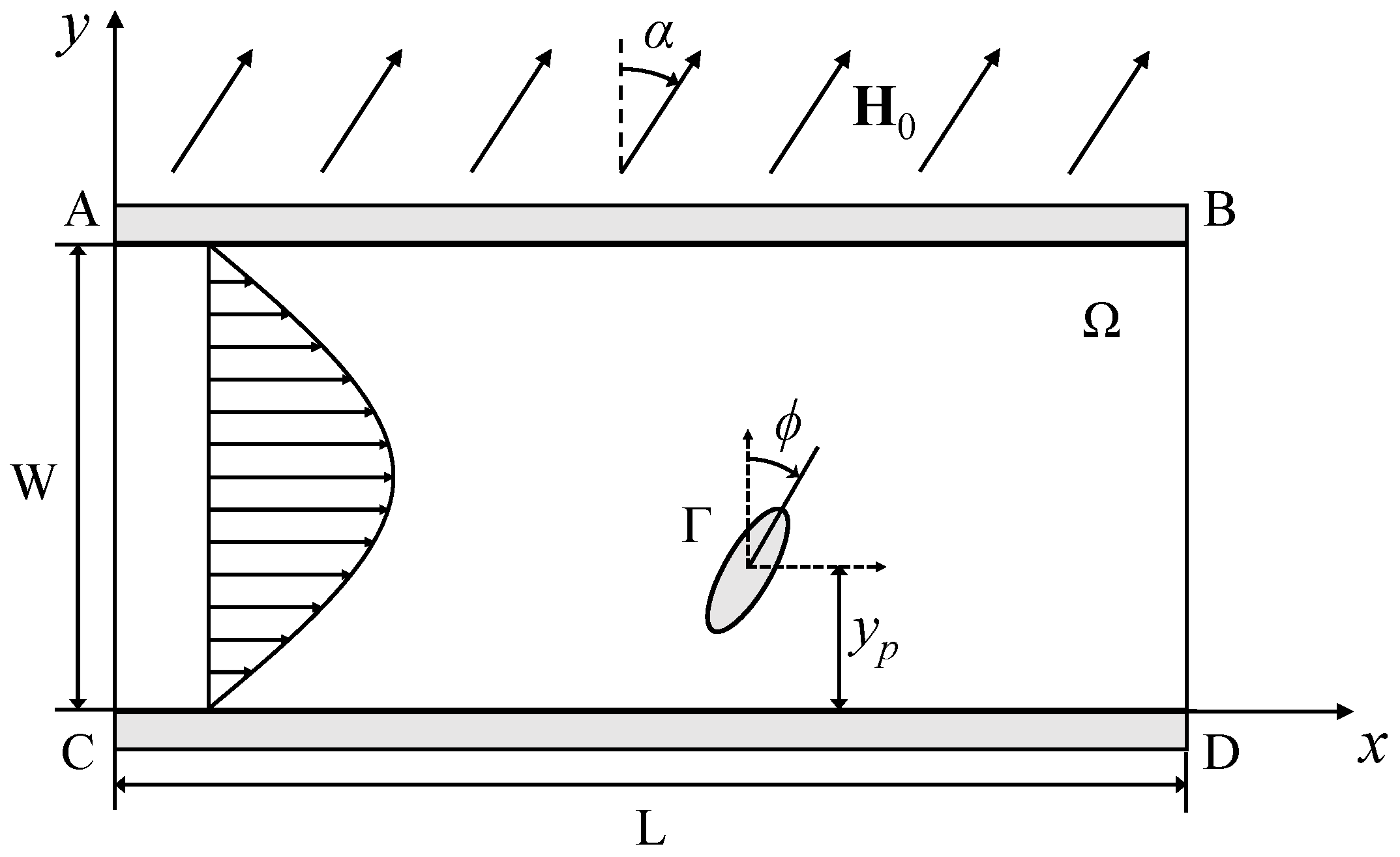
Figure 2.
Grid independence analysis: particle orientation as a function of time, for = 4, µm.
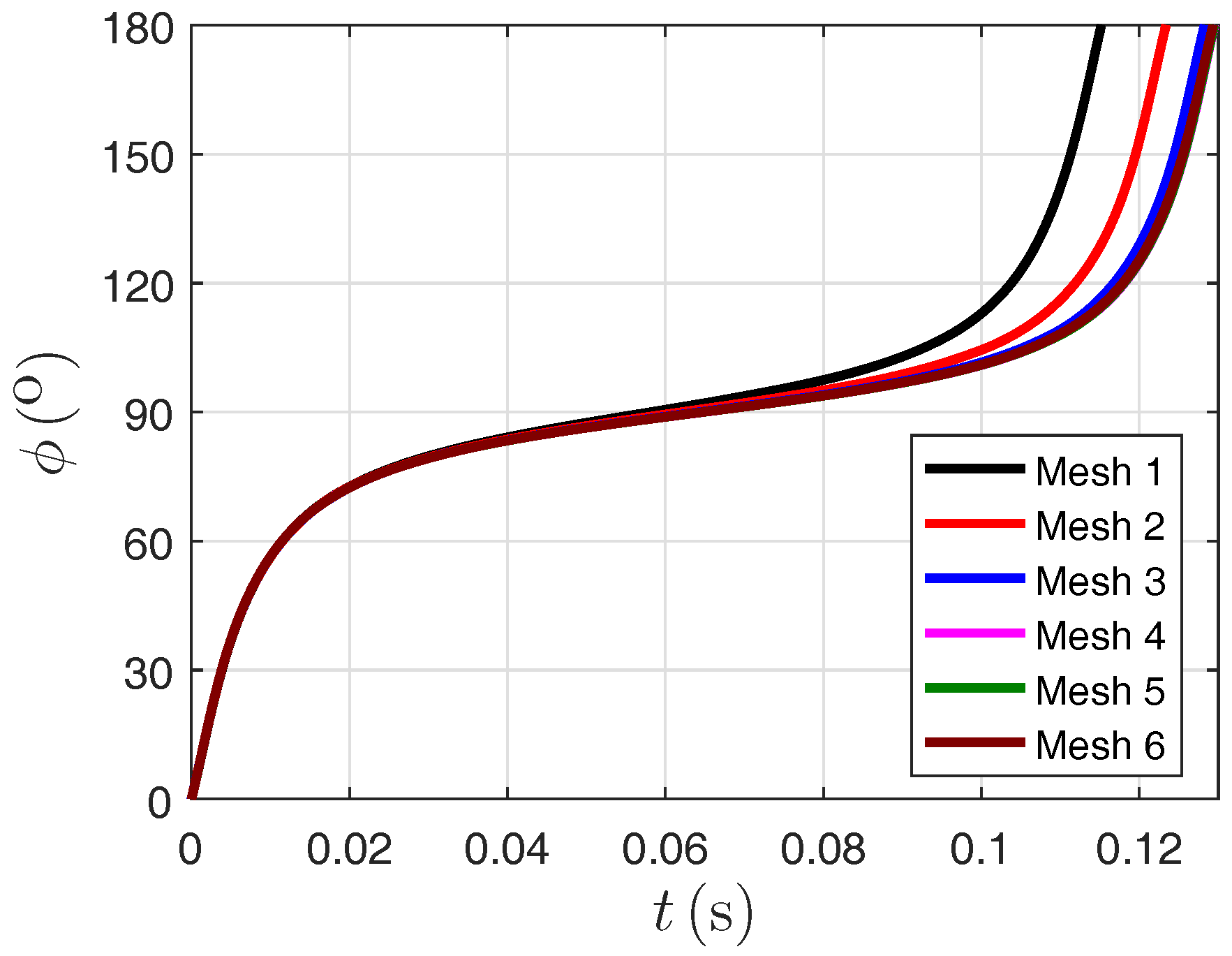
Figure 3.
Comparison between the finite element method (FEM) simulation and Jeffery’s theory on particle rotation.
Figure 3.
Comparison between the finite element method (FEM) simulation and Jeffery’s theory on particle rotation.
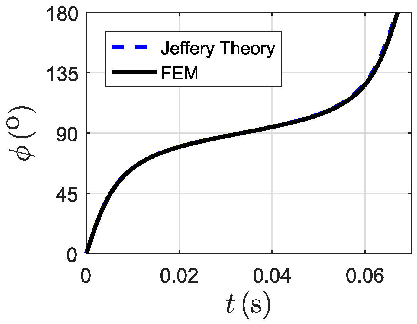
Figure 4.
Translation and rotation of the particle without a magnetic field. The particle () is initially located at µm. (a) trajectory of the particle over a rotation of 180°, with A denoting the amplitude of oscillatory motion; (b) the particle–wall separation distance over one period ; (c) the evolution of orientation angle, with the dimensionless time ; and (d) the rotational velocity versus .
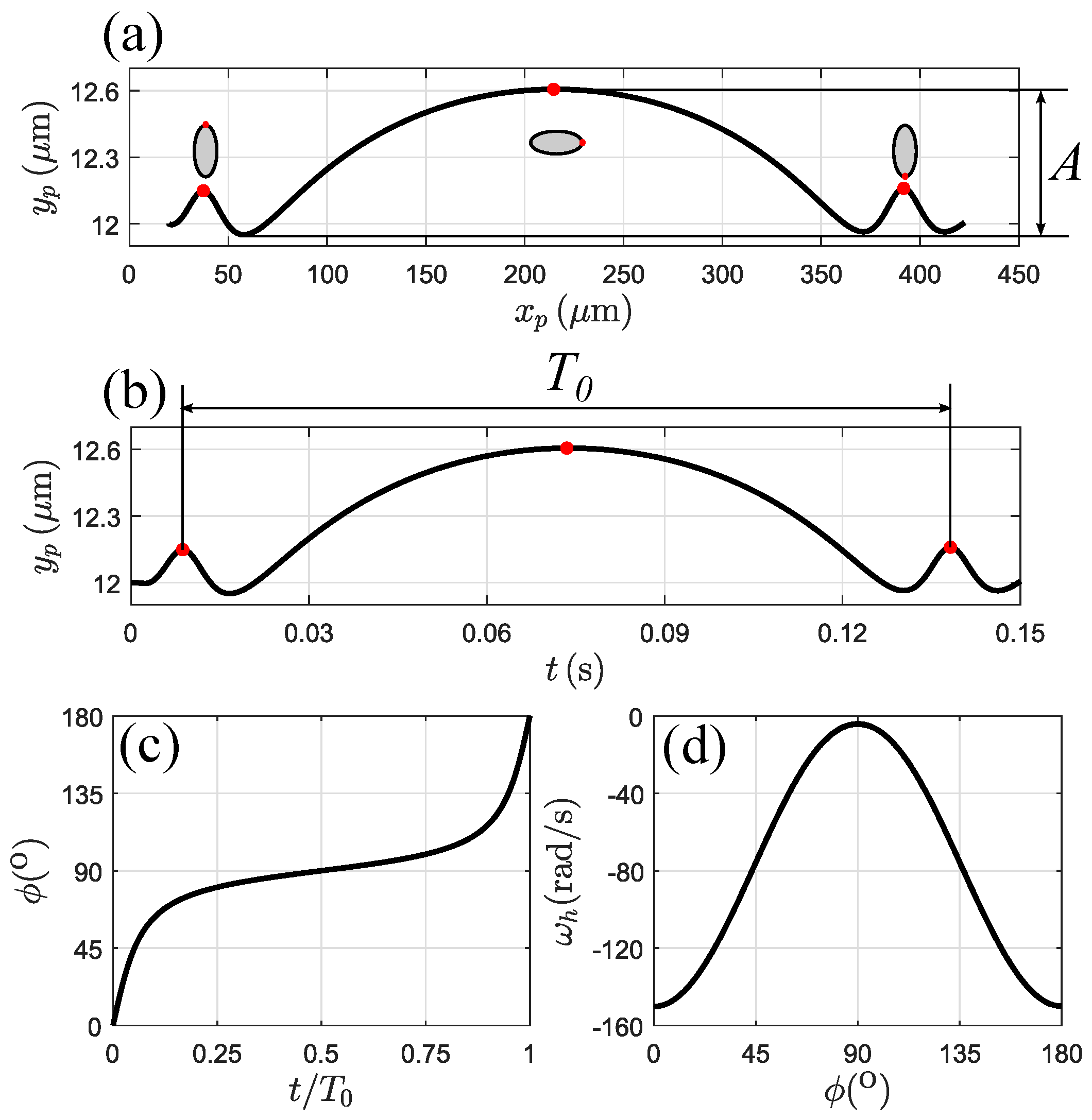
Figure 5.
The effects of initial position and particle aspect ratio on transport of elliptical particles without a magnetic field. (a) the effect on the lateral particle–wall separation: = 12 µm (solid line), 14 µm (dash line) and 16 µm (dash-dot line). The particle has a particle aspect ratio ; (b) the effect of particle aspect ratio on the lateral particle–wall separation distance: = 4 (solid line), = 3 (dash line), and = 2 (dash-dot line). The particles are initially located at = 12 µm; (c) dependence of amplitude of the oscillatory motion, A on ; and (d) the dimensionless period varies with dimensionless distance , for = 4 (circle), 3 (triangle), and 2 (rectangle). is the period of Jeffery’s orbit calculated by using the shear rate at the position of the particle centroid.
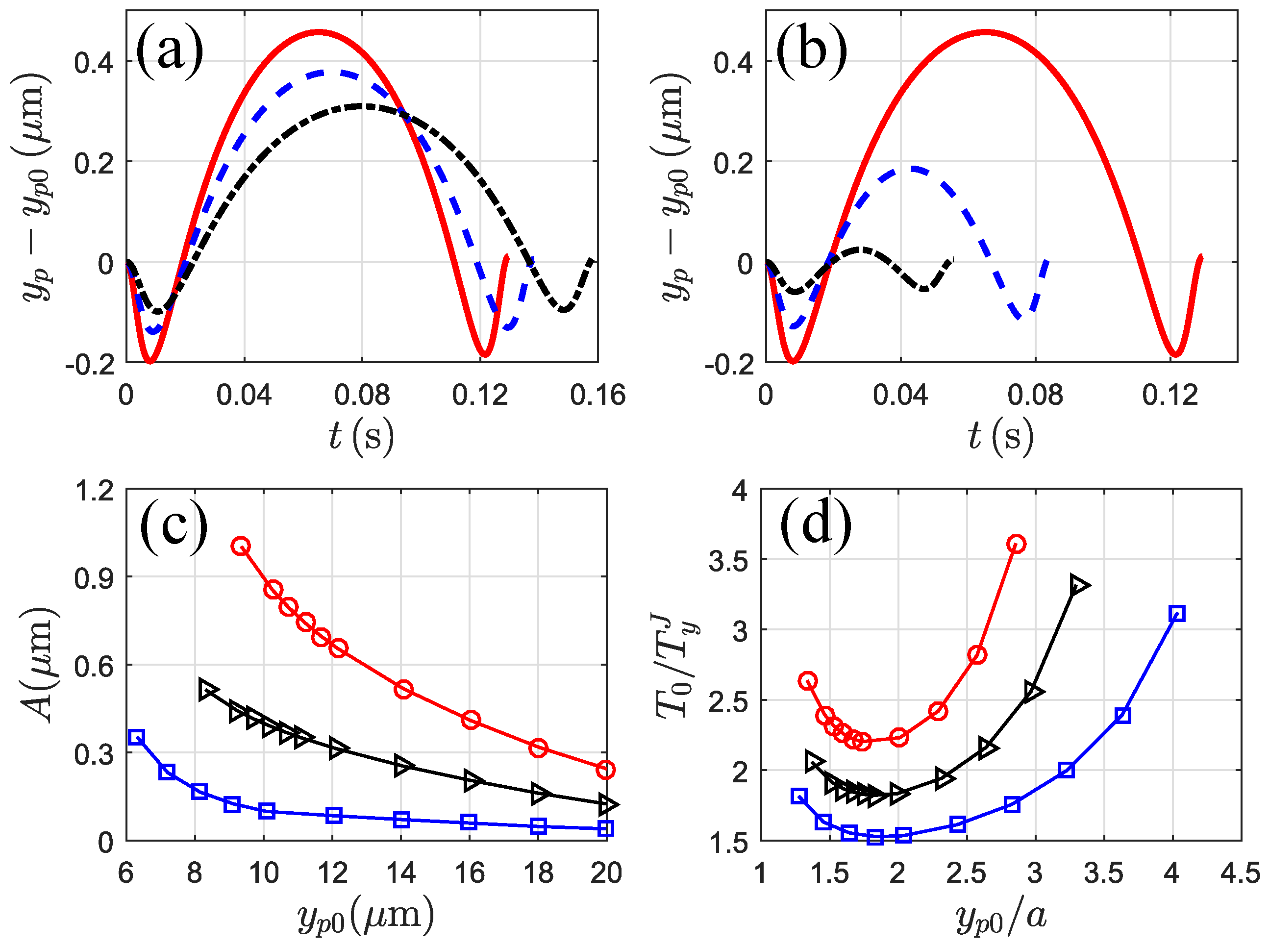
Figure 6.
Transport of the particle when the magnetic field is applied perpendicular to the flow direction, i.e., . The particle ( = 4) is initially located at = 12 µm. (a) the orientation angle, versus dimensionless time . A dimensionless time parameter is defined as the ratio of the time for the particle rotating from to to the period of rotation, T; (b) the particle–wall separation distance, as a function of time ( = 3000 A/m, ). denotes the net lateral migration of the particle over one period; (c) the rotational velocity versus : = 0 A/m (dash line), and 3000 A/m (solid line). The symmetry of particle rotational velocity about is broken, and .
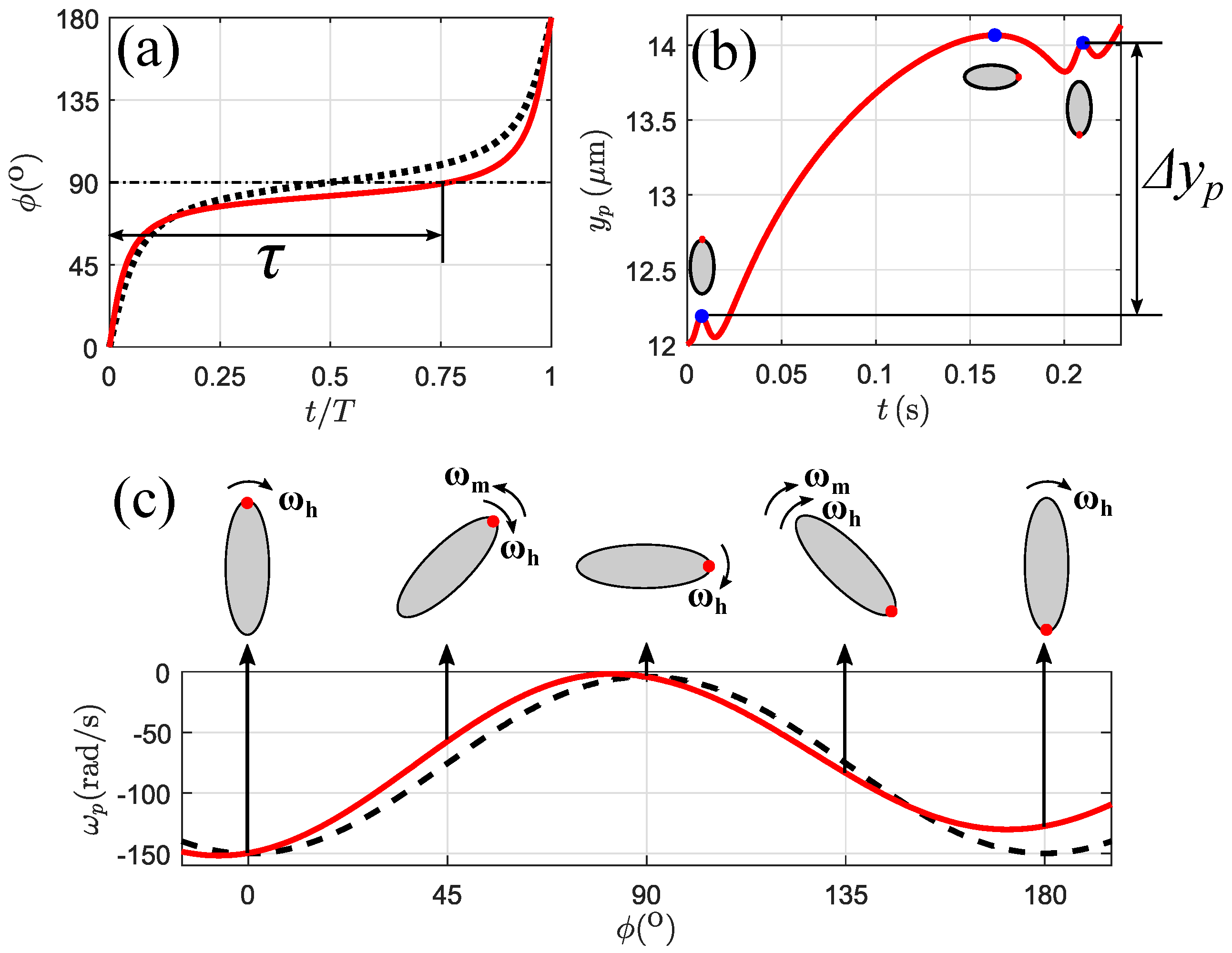
Figure 7.
The effect of magnetic field strength on particle transport, with = 4, = 12 µm, and . (a) versus time t over a period: = 0 (plus symbol), 1000 A/m (solid line), 2000 A/m (dash line), 3000 A/m(dash-dot line) and 4000 A/m (dot line); (b) varies with the magnetic field strength ; (c) the net migration of particle over a period: = 0 (solid symbol), 1000 A/m (circle symbol), 2000 A/m (square symbol), 3000 A/m (triangle symbol) and 4000 A/m (plus symbol); (b) the average vertical migration velocity varies with the magnetic field strength .
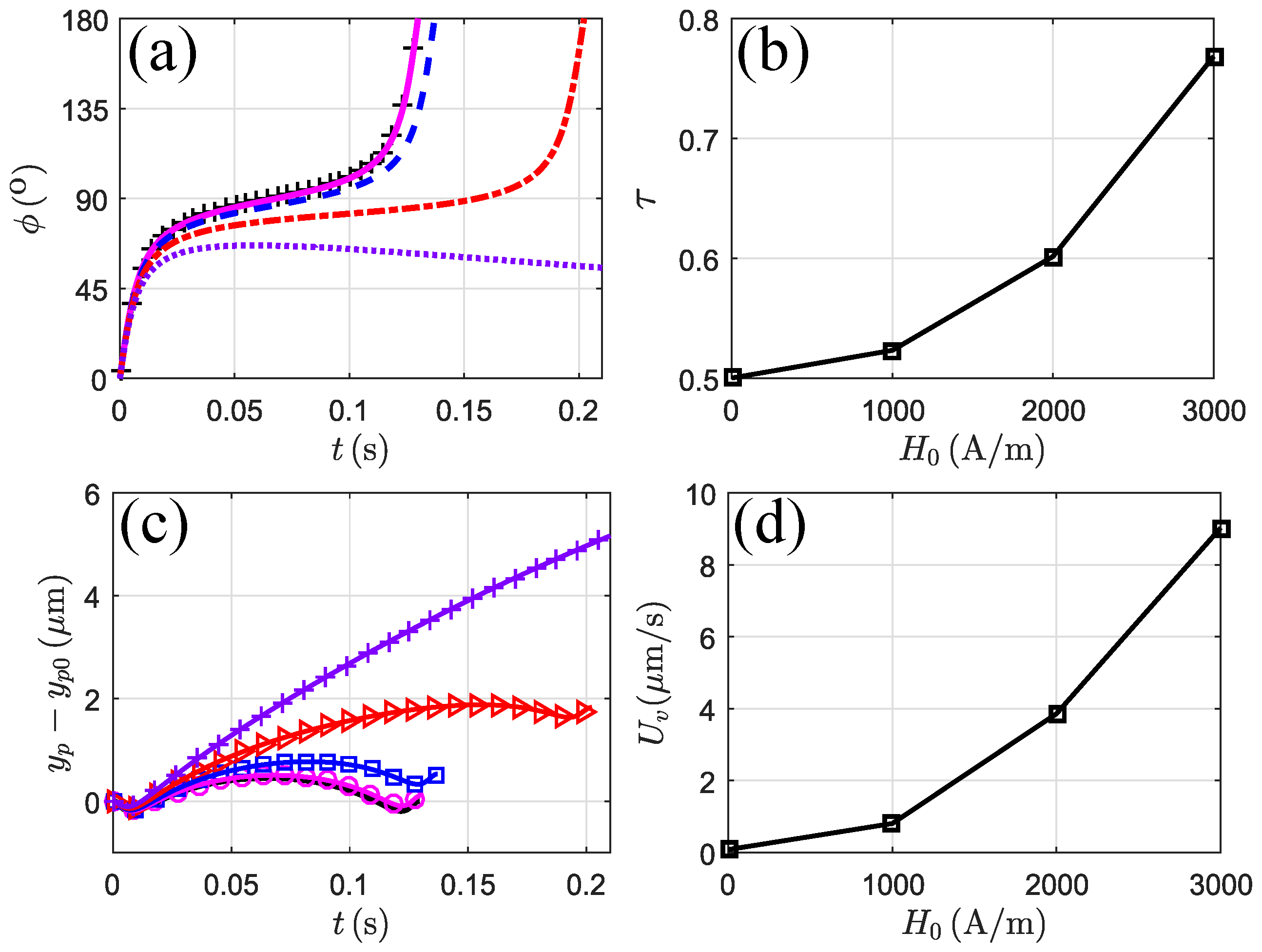
Figure 8.
Transport of the particle when the magnetic field is applied parallel to the flow direction, i.e., . The particle ( = 4) is initially located at = 12 µm. (a) varies with dimensionless time ; (b) variation of the particle–wall separation distance with time, and (c) the total rotational velocity varies with for = 0 A/m (dash line) and 3000 A/m (solid line).
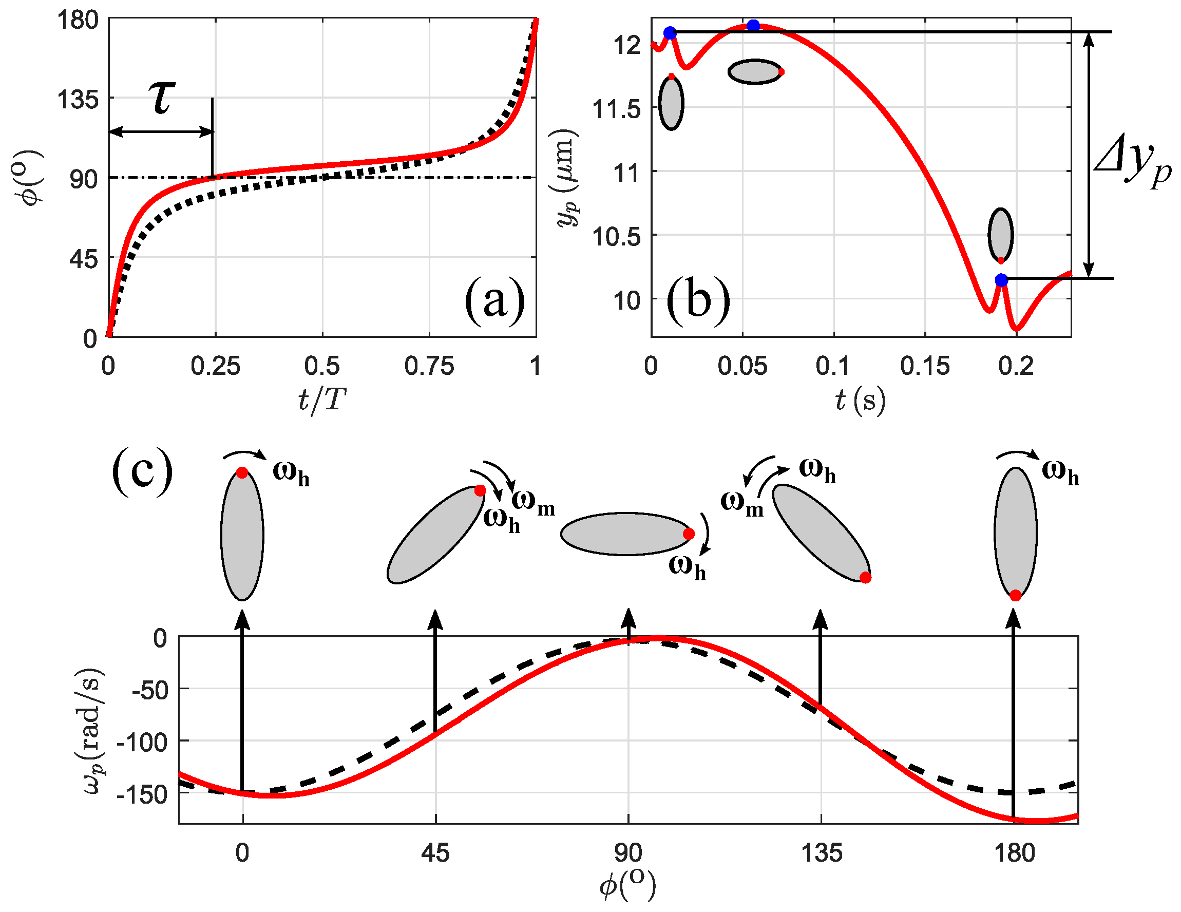
Figure 9.
The effect of magnetic field strength on particle transport, with = 4, = 12 µm, and . (a) versus t over a period for = 0 (plus symbol), 1000 A/m (solid line), 2000 A/m (dash line), 3000 A/m (dash-dot) and 4000 A/m (dot); (b) versus ; (c) the lateral migration of particle with time t over a period for = 0 (solid line), 1000 A/m (circle symbol), 2000 A/m (square symbol), 3000 A/m (triangle symbol) and 4000 A/m (plus symbol); (d) the vertical velocity versus magnetic field strength .
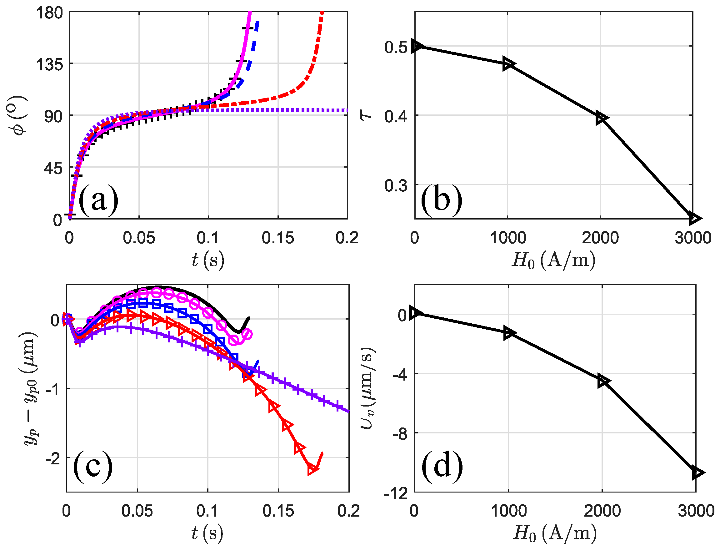
Figure 10.
Effect of the magnetic field when it is applied at . The particle ( = 4) is initially located at = 12 µm. (a) versus for = 0 (dash) and 3000 A/m (solid); (b) versus t over a period for = 0 (plus), 1000 A/m (solid), 2000 A/m (dash), 3000 A/m (dash-dot) and 4000 A/m (dot); (c) the dimensionless parameter as a function of ; (d) the migration of particle with time t over a period for = 0 (solid), 1000 A/m (circle), 2000 A/m (rectangle), 3000 A/m (triangle) and 4000 A/m (plus); and (e) dependence of lateral migration velocity on magnetic field strength .

Figure 11.
Effect of the magnetic field when it is applied at . The particle ( = 4) is initially located at = 12 µm. (a) the total rotational velocity versus for = 0(dash) and 3000 A/m (solid); (b) versus time t over a period for = 0 (plus), 1000 A/m (solid), 2000 A/m (dash), 3000 A/m (dash-dot) and 4000 A/m (dot); (c) the migration of particle as a function of t for = 0 (solid), 1000 A/m (circle), 2000 A/m (rectangle), 3000 A/m (triangle) and 4000 A/m (plus).

Figure 12.
Dependence of (a1) and (a2) on particle aspect ratio , with the particle is initially located at = 12 µm. Dependence of (b1) and (b2) on initial particle–wall separation distances when the particle aspect ratio is = 4. The magnetic field strength = 2000 A/m is applied at .
Figure 12.
Dependence of (a1) and (a2) on particle aspect ratio , with the particle is initially located at = 12 µm. Dependence of (b1) and (b2) on initial particle–wall separation distances when the particle aspect ratio is = 4. The magnetic field strength = 2000 A/m is applied at .
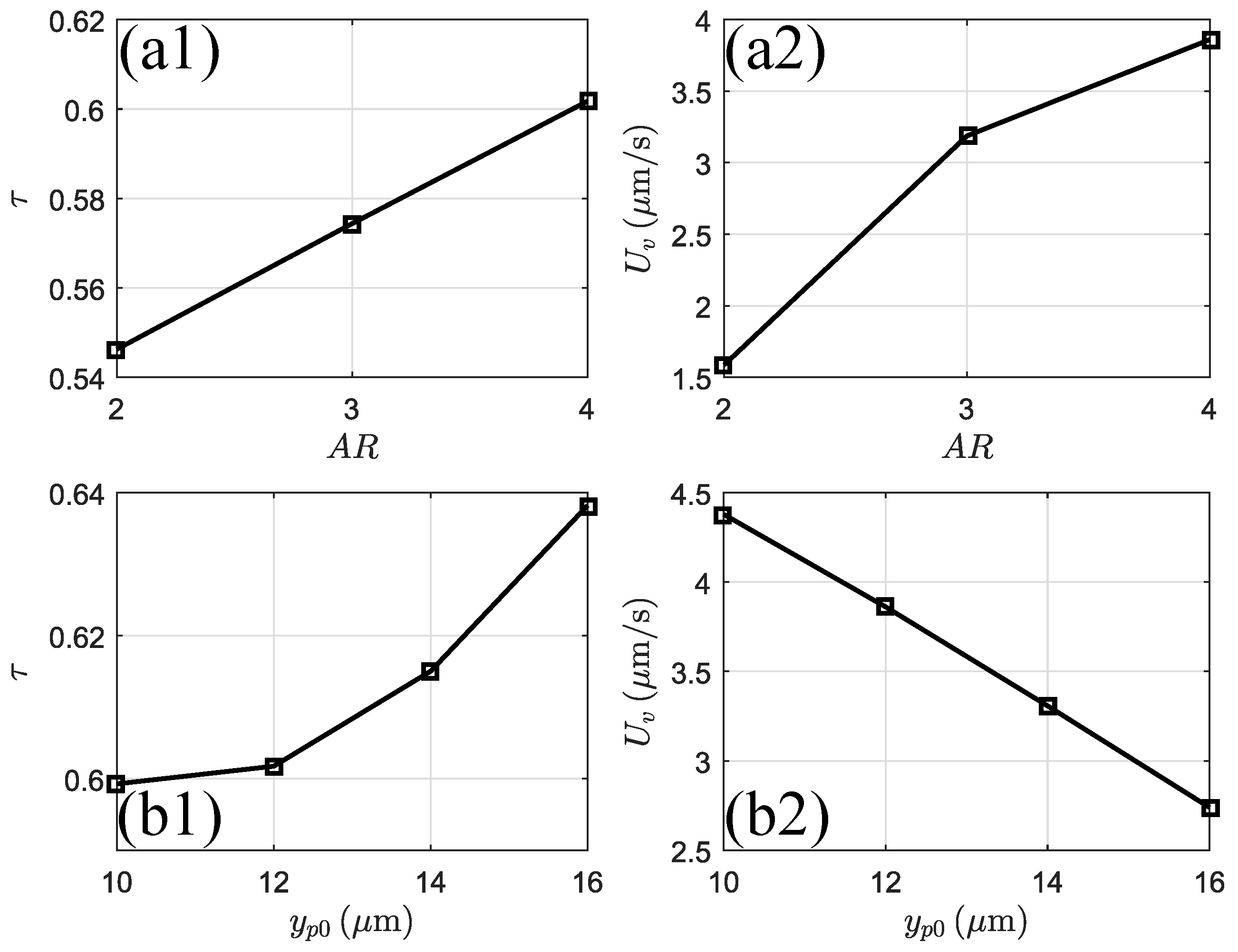
Figure 13.
The scaling relationship between and for (a); 3 (b); and 4 (c). The circle, square, triangle and star stands for numerical results of = 10 µm, 12 µm, 14 µm and 16 µm, respectively. The solid lines are the fitting results.
Figure 13.
The scaling relationship between and for (a); 3 (b); and 4 (c). The circle, square, triangle and star stands for numerical results of = 10 µm, 12 µm, 14 µm and 16 µm, respectively. The solid lines are the fitting results.

Table 1.
Six meshes for grid independence analysis.
| Mesh Sizes Used for Grid Independence Analysis | Domain Elements | Boundary Elements on Particle Surface |
|---|---|---|
| Mesh 1 | 6184 | 56 |
| Mesh 2 | 7794 | 68 |
| Mesh 3 | 8281 | 92 |
| Mesh 4 | 11,608 | 116 |
| Mesh 5 | 12,359 | 152 |
| Mesh 6 | 13,079 | 184 |
© 2018 by the authors. Licensee MDPI, Basel, Switzerland. This article is an open access article distributed under the terms and conditions of the Creative Commons Attribution (CC BY) license (http://creativecommons.org/licenses/by/4.0/).
Share and Cite
MDPI and ACS Style
Zhang, J.; Wang, C. Numerical Study of Lateral Migration of Elliptical Magnetic Microparticles in Microchannels in Uniform Magnetic Fields. Magnetochemistry 2018, 4, 16. https://doi.org/10.3390/magnetochemistry4010016
AMA Style
Zhang J, Wang C. Numerical Study of Lateral Migration of Elliptical Magnetic Microparticles in Microchannels in Uniform Magnetic Fields. Magnetochemistry. 2018; 4(1):16. https://doi.org/10.3390/magnetochemistry4010016
Chicago/Turabian StyleZhang, Jie, and Cheng Wang. 2018. "Numerical Study of Lateral Migration of Elliptical Magnetic Microparticles in Microchannels in Uniform Magnetic Fields" Magnetochemistry 4, no. 1: 16. https://doi.org/10.3390/magnetochemistry4010016
Note that from the first issue of 2016, this journal uses article numbers instead of page numbers. See further details here.