Passive Tracking of the Electrochemical Impedance of a Hybrid Electric Vehicle Battery and State of Charge Estimation through an Extended and Unscented Kalman Filter

Abstract

Estimation of a lithium battery electrical impedance can provide relevant information regarding its characteristics. Currently, electrochemical impedance spectroscopy (EIS) constitutes the most recognized and accepted method. Although highly precise and robust, EIS is usually performed during laboratory testing and is not suitable for any on-board application, such as in battery electric vehicles (BEVs) because it is an instrumentally and computationally heavy method. To address this issue and on-line system applications, this manuscript describes, as a main contribution, a passive method for battery impedance estimation in the time domain that involves the voltage and current profile induced by the battery through its ordinary operation without injecting a small excitation signal. This method has been tested on the same battery with different passive voltage and current profile and has been validated by achieving similar results. Compared to the original idea presented in the published conference paper, this manuscript explains, in detail, the previously developed method of transforming the battery impedance from the frequency domain to time domain. Moreover, this impedance measurement is used to estimate more robustly the battery state of charge (SoC) through Kalman filters. In the original published conference paper, only an extended Kalman filter (EKF) was applied. However, in this manuscript, an EKF and an unscented Kalman filter (UKF) are used and their performances are compared.

1. Introduction

Thanks to its advantageous characteristics, such as high energy and power density, long lifetime, low cost, and higher safety characteristics [1,2], lithium batteries are currently recognized as the most interesting technology for battery electric vehicles (BEVs). For such applications, it is crucial for both consumers and manufacturers to try to learn more about battery performance over its lifetime. This is why an efficient battery management system (BMS) [3,4] measures the main battery parameters, such as the temperature, the state of charge (SoC), the state of health (SoH), or the state of power (SoP) and how to avoid damage

To avoid damaging the battery, only noninvasive and nondestructive measurement processes are employed, and only external variables including the battery current, voltage and surface temperature [3,4,5,6] can be recorded over time. From these measurements, the battery electrochemical impedance can be estimated [7]. Battery impedance characterizes its dynamic behavior and is influenced by many factors such as the battery history, its polarization current, its SoC, its SoH, and its internal temperature. This explains why the battery electrochemical impedance is utilized in several approaches to evaluate the internal temperature [8,9,10], the SoC [11,12,13], and the SoH [13,14] of the managed battery.

The most accepted approach to estimate the battery impedance is electrochemical impedance spectroscopy (EIS) [15,16]. It is an active identification class method [17] and supposes the system to be LTI (Linear time invariant). It consists of exiting the battery through a current input composed of a unique sine wave with low amplitude and constant frequency, and recording the answering battery voltage output fluctuation. Then, the battery impedance can be estimated at the current sine wave frequency only. Finally, this measurement process is repeated to estimate the impedance for several frequencies. It is also possible to excite the battery through a current input composed of a sum of sines wave current with multiple discrete frequencies, measure answering battery voltage output fluctuation, and estimate the battery impedance for the corresponding discrete frequency bandwidth. Although very accurate, EIS is not applicable for an embedded system. In fact, advanced electronic generators are required to create sine waves with distinct frequencies or a multisine signal and so are responsible for a supplementary expense. Furthermore, this approach provides only one battery impedance estimation per measurement. As a consequence, every time a new impedance estimation is required, the entire measurement process has to be duplicated. It sharply reduces the ability to track the impedance over time.

Prediction of the battery behavior can be reached through modeling. In a prior publication [18] an invariant battery impedance model of a former Subaru BRZ 2015 converted into a Plug-in Hybrid Electric Vehicle (PHEV) has been developed. Nevertheless, it is written in [18] that the battery impedance model stays constant over the battery aging. Consequently, as the main contribution, this manuscript details a procedure that evaluates and revises regularly the PHEV battery impedance model during its lifetime. This strategy is similar to the one detailed in [19,20]. In contrast to [19,20], the method developed in this manuscript does not add a pseudo random binary signal (PRBS) to the battery current profile for evaluating its impedance and the impedance is computed in a time domain. Indeed, only the passive voltage and current induced by the battery, through its ordinary operation, are involved. This distinction makes our method more suitable for on-line system applications including the former Subaru BRZ 2015 converted into a PHEV. Compared to the original idea presented in the published conference paper [21], this manuscript explains, in detail, the previously developed method of transforming the battery impedance from frequency domain to time domain.

Using the estimated impedance computed by the proposed algorithm, another crucial state of the battery is then estimated: the SoC. In fact, a precise estimation of battery SoC is challenging, but it is necessary to overcome the “range anxiety” problem. This issue refers to the driver’s fear of running out of battery power on the road [22,23]. The first one is the range of an EV. In fact, the autonomy of electric varies from 100 miles for the most affordable car (Mitsubishi i-Miev) [24] to 335 miles for the most luxurious one (Tesla Model S) [25]. This fear comes from two factors. The second one is the lack of battery charging infrastructure. Both reasons lead to the necessity to predict the more accurately as possible the remaining range to prevent EVs from complete depletion on the road and leaving passengers stranded.

Nowadays, many methods have been developed and tested for SoC estimation. A recent journal article reviewed all of them in [26]. The most popular one is the Coulomb counting [27,28]. It consists of computing the remaining charge by integrating the current going into the battery over time. This is one of the most straightforward methods to embed in a vehicle. However, this methodology suffers from drift caused by the measurement noise and battery aging and requires knowledge of the initial SoC. Another well-known method is the voltage based SoC estimation, which infers SOC by an open circuit voltage (OCV)-SOC lookup table [29]. Unfortunately, OCV measurement requires an extended rest period before the terminal voltage reaches the actual OCV, which make this method unpractical. Many other works have been conducted using computational intelligence algorithms, such as fuzzy-logic [30], artificial neural networks (NNs) [31,32,33,34,35], and support vector machines (SVMs) [36,37,38]. These methods do not need expertise in battery modeling to be accurate. However, it requires many training data of all loading conditions, which can be time-consuming and potentially not provide adequate coverage for real-life applications. Electrochemical model-based methods have also recently been employed for SoC estimation [39,40,41]. Those techniques have the advantage to provide at the same time macroscopic quantities such as cell voltage and current but also microscopic quantities such as cell temperature, concentration, and potential. It allows to reflect more physically the chemical reaction happening inside a battery cell, such as the charge transfer and kinetic process. However, those methods require a high level of battery understandings and are computationally heavy making them unsuitable for BMS.

More recently, the development of model-based filtering methods [42,43,44,45,46,47,48,49,50] for establishing closed-loop estimation has been done. The impedance battery model and Coulomb counting model are employed to build a battery state-space model, where the current is utilized as the input, the voltage as the output, and the SoC as a hidden state. A filtering method including the extended or unscented Kalman filter (EKF and UKF), is then employed to estimate the SoC. Plett [42,43,44] presented an EKF filter for estimating the SoC of LiFePO₄ batteries. At each time point, the filter evaluates a voltage based on the system model and the recorded cumulative current. Then, the difference between the estimated and measured voltages serves to compute a correction term to adjust the SoC. However, an EKF is just a first order approximation, in the sense of Taylor series expansion, of a nonlinear model. The higher order terms are neglected, which can lead to significant errors for a nonlinear state-space model such as a battery. On the other hand, UKF is an upgraded version of EKF that uses an unscented transform, which computes statistics of a random variable propagating through a nonlinear system. In UKF, a set of sample points called sigma points represents the state distribution. The posterior mean and covariance of the state distribution, when propagated through the nonlinear system, are also captured by the propagated sigma points. UKF has been proven accurate to the third order, in the sense of Taylor series expansion, for any nonlinearity [51,52,53].

In every case, both EKF and UKF depend on the precision of the impedance battery model for estimating the battery SoC. Using the estimated impedance computed by the passive tracking impedance algorithm, the estimation of the battery SoC through Kalman filters can be more precise. In the original contribution of the published conference paper [21], only an EKF was applied. However, in this manuscript, the contribution has been extended by using an EKF and UKF and comparing their performance regarding the battery SoC estimation. The manuscript is organized as follows. In Section 2, the proposed approach is detailed, and the battery impedance estimation is validated by achieving similar results for the same battery using different passive voltage and current profile. Thereafter, in Section 3, using this estimated impedance an extended Kalman filter (EKF) and unscented Kalman filter (UKF) are applied to compute more robustly the battery SoC. Moreover, both filter performances are compared. The conclusion and future work are drawn in Section 4 and Section 5, respectively.

2. Impedance Estimation Method

The battery impedance estimation approach is explained in this section. This strategy, based on the Fourier transform and an exponential local averaging strategy, aims at tracking (precisely and regularly) the battery impedance over time. A similar method have already demonstrated accuracy to evaluate the lithium polymer battery impedance of a drone [19,20]. However, in this manuscript, the methodology is applied for a different battery chemistry (lithium iron phosphate), for a different application (a plug-in hybrid vehicle) and only uses the voltage and current profile induced by the battery during its ordinary operation without injecting a small excitation signal. Figure 1 summarizes the proposed method.

2.1. Linear and Time-Invariant Hypothesis

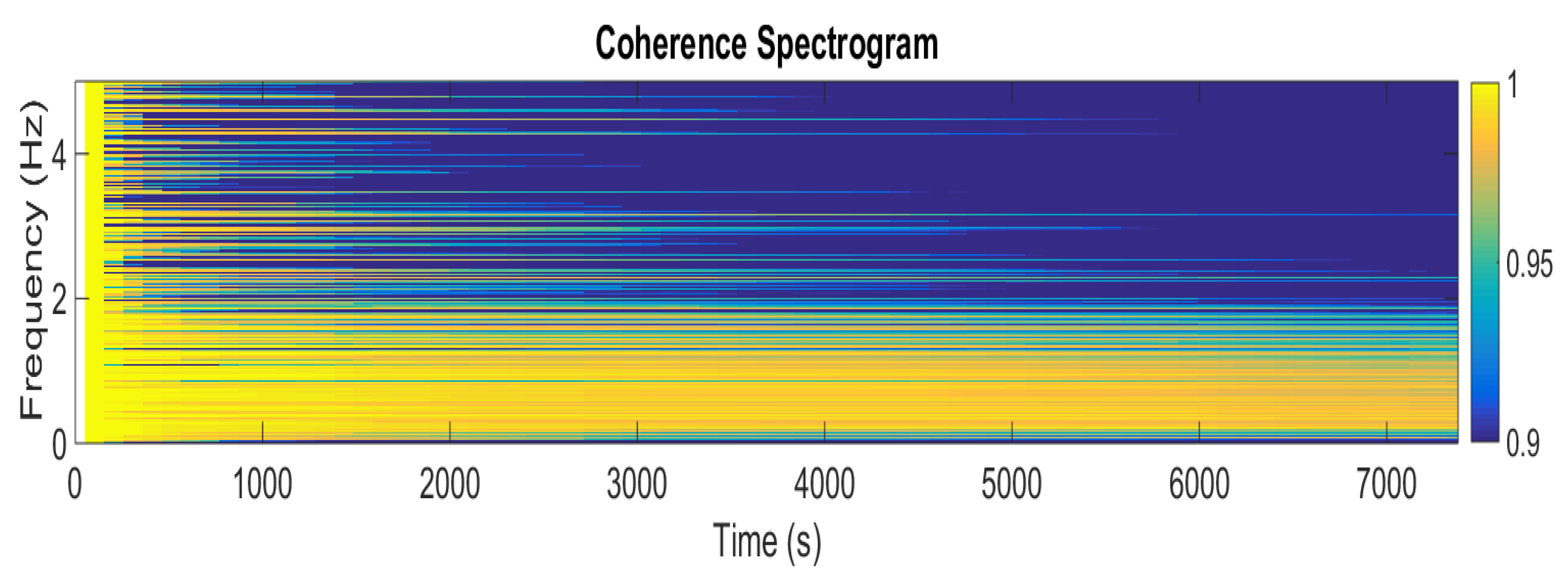
It is assumed that the parameters, on which the battery impedance characteristics depend stay invariant over the measurement process. Consequently, the battery can be regarded as a linear and time-invariant (LTI) system during the measurement time. Therefore, the estimated battery impedance ${\widehat{Z}}_k\left(f\right)$ can be determinde by Equation (1) [54,55].

$${\widehat{Z}}_k\left(f\right)=\frac{{\widehat{S}}_{u{i}_k}\left(f\right)}{{\widehat{S}}_{i{i}_k}\left(f\right)}$$

(1)

2.2. Coherence

To be able to apply this new impedance estimation method, the battery needs to be considered as an LTI system during the measurement time. To check this assumption, a statistical tool, called the squared spectral coherence, is used to ensure that the battery can be treated as an LTI system [56]. The estimated squared spectral coherence ${\widehat{C}}_{u{i}_k}\left(f\right)$ between the current i(t) and the voltage u(t) is provided in Equation (2) where ${\widehat{S}}_{u{u}_k}\left(f\right)$ is the estimated power spectral density (PSD) of the voltage.

$${\widehat{C}}_{u{i}_k}\left(f\right)=\frac{{\left|{\widehat{S}}_{u{i}_k}\left(f\right)\right|}^2}{{\widehat{S}}_{u{u}_k}\left(f\right){\widehat{S}}_{i{i}_k}\left(f\right)}$$

(2)

${\left|{\widehat{C}}_{u{i}_k}\left(f\right)\right|}^2$ belongs to [0, 1]. If ${\left|{\widehat{C}}_{u{i}_k}\left(f\right)\right|}^2$ is equal to one for a given frequency band, the system can be treated as LTI for this frequency band, and, consequently, the impedance can be computed using Equation (1). Conversely, if ${\left|{\widehat{C}}_{u{i}_k}\left(f\right)\right|}^2$ tends toward 0, either measurements are highly polluted by noises or the system cannot be regarded as LTI. Therefore, the impedance cannot be calculated by Equation (1). In reality, the squared spectral coherence is never equal to one, but it can be very close. For the purpose of this manuscript, it has been decided that the battery is considered as an LTI system for a given frequency and during the measurement time, if the squared spectral coherence is superior to 0.99.

2.3. Impedance Estimation in Frequency Domain

To estimate ${\widehat{Z}}_k\left(f\right)$ and ${\left|{\widehat{C}}_{u{i}_k}\left(f\right)\right|}^2$, we first calculate the PSD ${\widehat{S}}_{i{i}_k}\left(f\right)$, ${\widehat{S}}_{u{u}_k}\left(f\right)$ and the coherence power spectral density (CPSD) ${\widehat{S}}_{u{i}_k}\left(f\right)$.

Using a time window, the data are seperated into blocks, and the Fast Fourier transform algorithm is used to calculate their discrete Fourier transform (DFT). The different steps of this method are provided in Figure 1. The block length has to be large enough for evaluating ${\widehat{Z}}_k\left(f\right)$ on the widest frequency band as possible, and short enough for considering the battery as an LTI system during the measurement time. In this study, a hamming window of 1024 points has been selected.

After an initialization step, a recursive equation, implementing an exponential averaging approach using a forgetting factor $\alpha$ = 0.9, enable the battery impedance and the coherence to be revised at each new data block. Such strategy has been selected because it allows to set the trade-off between estimation performance and implementation complexity through the forgetting factor. Moreover, the forgetting factor also allows us to set the trade-off between the convergence time and the final estimation error: the smaller the convergence time is, the higher the final estimation error is and conversely. Equations (3) and (4) provide the algorithm necessary to evaluate the CPSD ${\widehat{S}}_{u{i}_k}\left(f\right)$ recursively.

$${\widehat{P}}_{u{i}_k}\left(f\right)=A{V}_k\left(f\right) I_k^{*}\left(f\right)$$

(3)

$${\widehat{S}}_{u{i}_k}\left(f\right)=\alpha {\widehat{S}}_{u{i}_{k-1}}\left(f\right)+\left(1-\alpha \right) {\widehat{P}}_{u{i}_k}\left(f\right)$$

(4)

where A is a normalization factor, * denotes complex conjugation, and V_k(f) (I_k(f) respectively) is the DFT of the kth block of voltage (current respectively) sample, and $\alpha$ is the forgetting factor, that belongs to [0, 1]. In this equation, the estimated cross periodogram between the kth blocks of voltage and current samples is noted ${\widehat{P}}_{u{i}_k}\left(f\right)$. Finally, the battery impedance is evaluated by dividing the estimated CPSD by the PSD of the current (Equation (1)).

2.4. Impedance Estimation in Time Domain

To estimate ${\widehat{Z}}_k\left(t\right)$, we need first to select an impedance battery model order. For automotive application, an n order Resistance/Capacitor network, as shown in Figure 2, is commonly used to model the battery impedance [57,58,59].

The equation of such impedance is described by Equation (5)

$${\widehat{Z}}_n\left(s\right)=\frac{{{\displaystyle \sum }}_{m=0}^n{\widehat{b}}_n\left(i\right)s^{n-m}}{{{\displaystyle \sum }}_{m=0}^n{\widehat{a}}_n\left(i\right)s^{n-m}}$$

(5)

where ${\widehat{Z}}_n\left(s\right)$ is the estimated impedance in the Laplace domain, s = 2πf, f is the frequency in Hz, n is the order of the battery model, ${\widehat{b}}_n$ and ${\widehat{a}}_n$ are the estimated real coefficient of the numerator and denominator, respectively. To estimate such coefficients, the Matlab function ‘invfreqs’ is used [60], as shown in Equation (6).

$$[{\widehat{b}}_n,{\widehat{a}}_n\left]=invfreqs\right[{\widehat{Z}}_n\left(s\right),f,n,n]$$

(6)

Then, to estimate the value of the RC network parameters, a partial fraction decomposition is computed by using the Matlab function ‘residue’ [61].

$$[{\widehat{r}}_n,{\widehat{p}}_n,{\widehat{d}}_n\left]=residue\right[{\widehat{b}}_n,{\widehat{a}}_n]$$

(7)

The computation of ${\widehat{r}}_n$, ${\widehat{p}}_n$ often provides complex conjugate numbers, which are not desirable values because the parameters of the RC networks should be real values. To overcome this issue, the modulus value of those complex numbers is taken. As those complex numbers are necessarily complex conjugate because the original quotient polynomial provided in Equation (5) uses real coefficient only, many RC branches have the same parameters values, which lead to a reduction of the battery model order.

Then the final parameters are computed through those following equations:

$${\widehat{R}}_s\left(n\right)={\widehat{d}}_n$$

(8)

$${\widehat{R}}_m\left(n\right)=\left|{\widehat{r}}_n\left(m\right)\right|/\left|{\widehat{p}}_n\left(m\right)\right|$$

(9)

$${\widehat{C}}_m\left(n\right)=1/\left({\widehat{R}}_m\left(n\right) \left|{\widehat{p}}_n\left(m\right)\right|\right)$$

(10)

$${\widehat{Z}}_n\left(f\right)={\widehat{R}}_s+{\displaystyle \sum }_{i=0}^n\frac{{\widehat{R}}_i\left(n\right)}{1+{\widehat{R}}_m\left(n\right) {\widehat{C}}_m\left(n\right)2\pi jf}$$

(11)

In this manuscript, this process is repeated for every positive natural number n lower than 40. The number 40 is large enough to cover different order of impedance battery model for an automotive application [57,58,59]. However, it can be selected as need be. Then, a decision to select the battery model order is made based of the Root Mean Square Error (RMSE) between the modulus and phase of ${\widehat{Z}}_n\left(f\right)$ and ${\widehat{Z}}_k\left(f\right)$ are calculated in Equations (12) and (13).

$$RMS{E}_{Pi}=\sqrt{\frac{{{\displaystyle \sum }}_{i=1}^l{\left(arg\left[{\widehat{Z}}_k\left(f\right)\right]-arg\left[{\widehat{Z}}_i\left(f\right)\right]\right)}^2}{l}}$$

(12)

$$RMS{E}_{Mi}=\sqrt{\frac{{{\displaystyle \sum }}_{i=1}^l{\left(\left|{\widehat{Z}}_k\left(f\right)\right|-\left|{\widehat{Z}}_i\left(f\right)\right|\right)}^2}{l}}$$

(13)

where $RMS{E}_{Pi}$ and $RMS{E}_{Mi}$ are respectively the phase and modulus RMSE of the “i” order impedance battery model, m is the number of sample of the estimated impedance ${\widehat{Z}}_k\left(f\right)$.

Once the choice of the battery model is made, ${\widehat{Z}}_k\left(t\right)$ is computed as follow.

$${\widehat{V}}_m\left(t\right)=T_s\left[\frac{i_k\left(t-T_s\right)}{{\widehat{C}}_m}-\frac{V_m\left(t-T_s\right)}{{\widehat{R}}_m{\widehat{C}}_m}\right]+{\widehat{V}}_m\left(t-T_s\right)$$

(14)

$$\begin{array}{c}{\widehat{Z}}_k\left(t\right)={\widehat{R}}_S+\frac{{{\displaystyle \sum }}_{m=1}^n{\widehat{V}}_m\left(t\right)}{I_k\left(t\right)}\end{array}$$

(15)

where T_S stands for the sampling period.

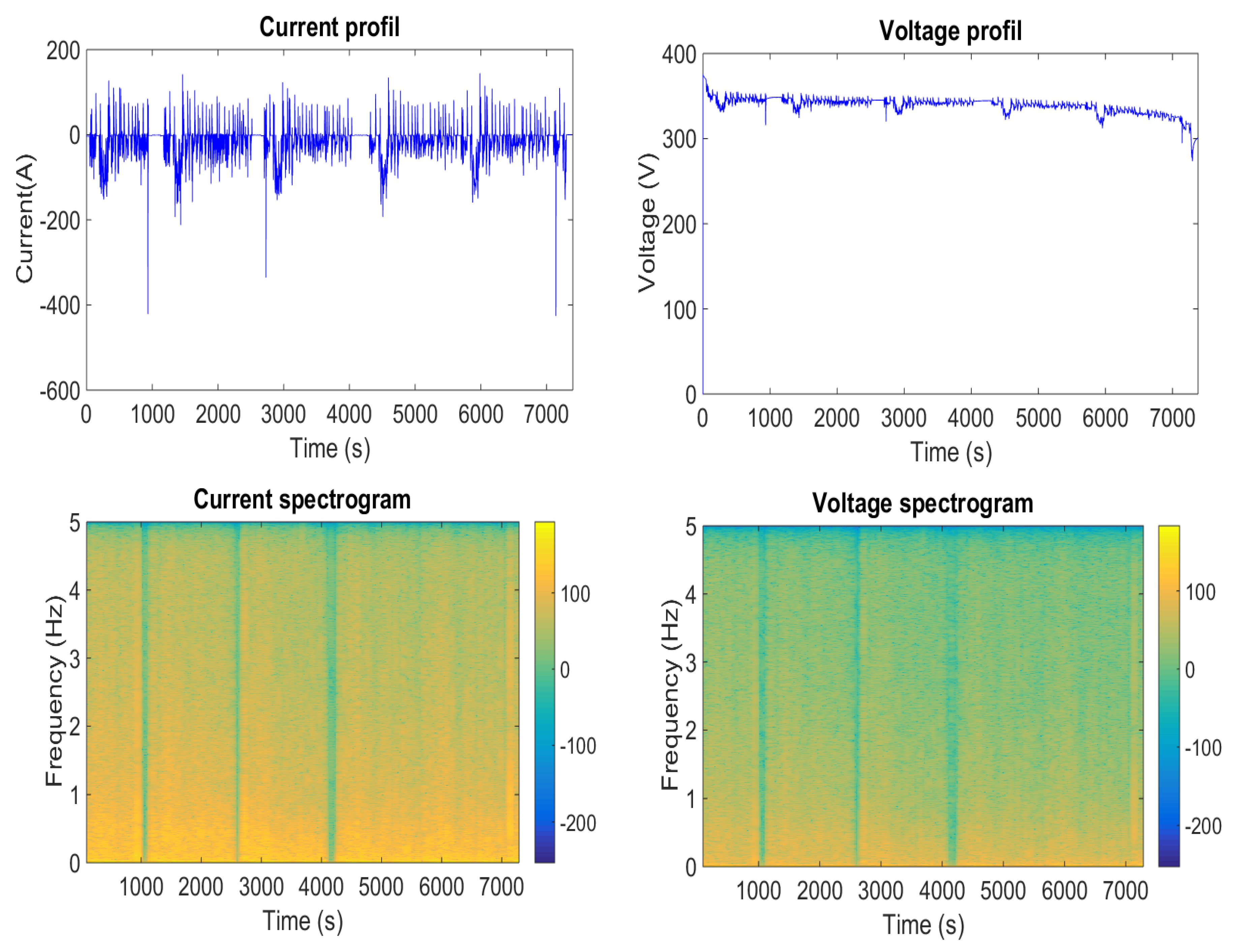
2.5. Experimental Protocol

The vehicle shown in Figure 3 has been already described in [62,63,64,65]. It is a series PHEV and its powertrain is composed of an electric generator, an Energy Storage System (ESS) made of a lithium iron phosphate battery, and an electric motor connected to a DC bus. The schematic and specifications of the vehicle model are given in Figure 4 and

Table 1. Specification of power-train components of the plug-in hybrid electric vehicle (PHEV).

Power-Train Components	Name	Characteristics
Energy Storage System (ESS)	Lithium iron phosphate (LFP) prismatic cells from A123	Capacity = 39.2 Ah; nominal voltage = 340 V; nominal energy = 13.3 kWh; configuration: 7 × 15s2p.
Internal Combustion Engine (ICE)	Model MPE850 from Weber	41 kW, 2 cylinders, 850 cc.
Electric Generator	Model YASA-400	93 kW, axial flux permanent magnet.
Electric Motors Unit	Model GVK210-100L6 from Linamar	2 × 80 kW, unit ratio = 8.49.
Vehicle dynamics	2015 Subaru BRZ Limited	Drag coefficient = 0.28; frontal area = 1.9695 m2; PHEV mass = 1300 kg; wheel radius = 0.3 m.

.

The car has been run through repetition of many HWFET (highway) and UDDS (urban) drive cycles from full battery charge (respectively, 96% and 100% of SoC) to its complete depletion (5% of SoC) on a dynamometer. During the experiment, the speed of the car was controlled by a human driver operating an accelerator and brake pedal. The driver tried to follow the UDDS and HWFET drive cycle as closely as possible, but pedal sensitivity limitation and small interruption between some drive cycles repetition makes it difficult. Moreover, the tests may have been stopped before finishing a complete cycle because the battery was depleted. However, the vehicle speed profile does not have to exactly follow the drive cycle to test accurately the battery impedance estimation algorithm. Those experiments aim at providing the passive voltage and current profile of the battery while the vehicle is running. Even if the sampling frequency for this test looks small (only 20 Hz), previous literature [66,67,68,69] supports that this sampling frequency is adequate for estimating the battery impedance for automotive applications. Furthermore, the identified battery bandwidth for the impedance model described in [18] is between 0.0008799 Hz and 0.02134 Hz. Consequently, it can be concluded the sampling frequency of 20 Hz is large enough.

2.6. Results and Discussion

The voltage and current profile and their associated spectrogram during UDDS are showed in Figure 5. The coherence spectrogram during UDDS is provided in Figure 6. It has been defined that the coherence has to be greater than 0.99 to consider the battery as an LTI system and so to update the prior the battery impedance estimation. As expected with a sampling frequency of 20 Hz, the voltage and coherence spectrograms suggest that the frequency content of the signal is mainly contained from 0 to 2 Hz. The same conclusion is achieved during HWFET.

As the Figure 5 and Figure 6 show that the signal content is included up to a maximum frequency of 2 Hz, ${\widehat{Z}}_k\left(f\right)$ is estimated from 0 to 2 Hz during UDDS and HWFET. Then, the different ${\widehat{Z}}_n\left(f\right)$ depending the order “n” of the impedance battery model is computed, and the modulus and phase RMSE are plotted in Figure 7.

From Figure 7, it can be observed that for “n” lower than 21, the modulus and phase RMSE are quite constant and lower than for “n” higher than 21. In fact, as this method estimates impedance in a discrete frequency domain, above a certain order, too many resistance and capacitance needs to be computed for the number of available frequency points estimated. This is why any impedance battery model order lower than 21 can be selected. In this manuscript, n has been selected so as the battery model order is the same as the model developed in [18]. As during the partial fraction decomposition, complex conjugate numbers are derived, the absolute values of those numbers lead to a reduction of the impedance battery model order. This is why n_s equal to three has been selected.

Table 2. Characteristics of the battery impedance.

Parameter	UDDS	HWFET
${\widehat{R}}_s$	0.0873 Ω	0.0865 Ω
${\widehat{R}}_1$	0.0014 Ω	0.0026 Ω
${\widehat{C}}_1$	0.4187 kF	0.2467 kF
${\widehat{R}}_2$	0.2743 Ω	0.2621 Ω
${\widehat{C}}_2$	0.410 kF	2.065 kF

provides the different capacitance and resistance values of the battery impedance model estimated through the passive UDDS and HWFET current and voltage profiles. Figure 8 shows, respectively, the Bode diagrams of ${\widehat{Z}}_k\left(f\right)$ and ${\widehat{Z}}_3\left(f\right)$.

From Table 2, it can be noticed that ${\widehat{R}}_s$ values are close to each other. Moreover, the sum of each resistance in each case is a similar value (around 0.34 Ω), and also the time constant ${\widehat{R}}_1{\widehat{C}}_1$ is about the same value (0.6 s) for UDDS and HWFET testing.

Concerning the battery impedance estimation during both drive cycles, it has been realized on the same battery, and it can be considered that its aging between both experiments has not changed. Nevertheless, the external battery temperature has changed during the testing: from 26.5 °C to 38.5 °C for UDDS and from 25 °C to 38.5 °C for HWFET. Furthermore, durations of the drive cycles tests are different: 7381 s for the UDDS for only 3056 s for the HWFET. Therefore, during the UDDS drive cycle, more data have been gathered to update more precisely the battery impedance potentially. Consequently, both estimated impedances are not identical, but still very similar as shown in Figure 8 and Table 2.

3. SoC Estimation through EKF and UKF

3.1. Overview

For the nonlinear model, the EKF and UKF methods are proposed, respectively, in [42,43,44,51,52,53,70,71,72]. The nonlinear model can be linearized by Taylor expansion to the first order for EKF and the third order for the UKF, and then SoC estimation can be estimated by using the original Kalman filter. Linear discrete state-space equations are provided in Equations (16) and (17).

$$x_{k+1}=g\left(x_k,u_{k+1}\right)+w_k$$

(16)

$$y_k=h(x_k,u_k)+v_k$$

(17)

Here, $x_k$ and $u_k$ are respectively the system status vector and the input vector at time k, g corresponds to the linearized transfer function matrix of the nonlinear status and h corresponds to the linearized matrix of the nonlinear measurement function, w_k and v_k are, respectively, the system noise and the measurement noise, whose covariances are Q_k and R_k.

$$E\left\{w_k\times w_k^T\right\}=Q_k$$

(18)

$$E\left\{v_k\times v_k^T\right\}=R_k$$

(19)

In the case of battery SoC estimation, the linear discrete state space equation can be expressed by the following equations.

$${\widehat{SoC}}_{k+1}={\widehat{SoC}}_k+\frac{I_k{T}_s}{C_n}+w_k$$

(20)

$${\widehat{V}}_k=V_{oc}\left({\widehat{SoC}}_k\right)+{\widehat{Z}}_k{I}_k+v_k$$

(21)

3.2. EKF Algorithm

Recursive steps of the EKF algorithm can be summarized as follows:

(1)

Initialize the original parameters

$$x_0=E\left\{x\left(0\right)\right\}$$

(22)

$$P_0=E\{\left[x\left(0\right)-E\left\{x\left(0\right)\right\}\right]{\left[x\left(0\right)-E\left\{x\left(0\right)\right\}\right]}^T\}$$

(23)

(2)

Estimate the predicted state

$${\overline{x}}_{k+1}=g\left(x_k,u_{k+1}\right)$$

(24)

(3)

Update the estimated covariance

$${\overline{P}}_{k+1}=F_{k+1}{P}_k{F}_{k+1}^T+Q_{k+1}$$

(25)

(4)

Compute the near-optimal Kalman gain

$$K_k={\overline{P}}_{k+1}{H}_k^T{(R_k+H_k{P}_k{H}_k^T)}^{-1}$$

(26)

(5)

Update the estimated state

$$x_{k+1}={\overline{x}}_{k+1}+K_{k+1}(y_{k+1}-h\left({\overline{x}}_{k+1},u_{k+1}\right))$$

(27)

(6)

Predict the estimated covariance

$$P_{k+1}=\left(I-K_{k+1}{H}_{k+1}\right){\overline{P}}_{k+1}$$

(28)

(7)

Repeat the recursive filter calculation from step 2 to 6.

For this manuscript the following parameters values have been selected: $P_0=\left[\begin{array}{ccc}{10}^{-6}& 0& 0\\ 0& 1& 0\\ 0& 0& 1\end{array}\right]$, $Q_k=\left[\begin{array}{ccc}{10}^{-8}& 0& 0\\ 0& 1& 0\\ 0& 0& 1\end{array}\right]$, $R_k$ = 10, $H_k=\left[\frac{d\left(V_{oc}\right)}{dSoC} 1 1\right]$.

3.3. UKF Algorithm

Recursive steps of UKF algorithm can be summarized as follows:

(1)

Initialize the original parameters are the same as Equations (22) and (23).

(2)

For k $\in \left[\left|1;+\infty \right|\right],$ calculate the sigma points for the state model

$${\sigma }_k=\left[x_k, x_k+\sqrt{\left(L+\lambda \right)P_k}, x_k-\sqrt{\left(L+\lambda \right)P_k}\right]$$

(29)

$$\lambda =3{\gamma }^2-L$$

(30)

where L is the length of $x_k$ and $\gamma$ is a scaling parameter that determines the spread of the sigma points around $x_k$.

(3)

Propagate the sigma points through the state model

$${\overline{\sigma }}^{\prime }{}_{k+1}=g\left({\sigma }_k,u_{k+1}\right)$$

(31)

(4)

Calculate the propagated mean

$${\overline{x}}_{k+1}={\displaystyle \sum }_{i=0}^{2n}{\omega }_m\left(i\right){\overline{\sigma }}^{\prime }{}_{k+1}\left(i\right)$$

(32)

(5)

Calculate the propagated covariance

$${\overline{P}}_{k+1}={\displaystyle \sum }_{i=0}^{2n}{\omega }_c\left(i\right)\left[{\overline{\sigma }}^{\prime }{}_{k+1}\left(i\right)-{\overline{x}}_{k+1}\right]{\left[{\overline{\sigma }}^{\prime }{}_{k+1}\left(i\right)-{\overline{x}}_{k+1}\right]}^T+Q_{k+1}$$

(33)

(6)

For k $\in \left[\left|1;+\infty \right|\right],$ calculate the sigma points for the measurement function

$${\overline{\sigma }}_{k+1}=\left[{\overline{x}}_{k+1}, {\overline{x}}_{k+1}+\sqrt{\left(L+\lambda \right){\overline{P}}_{k+1}}, {\overline{x}}_{k+1}-\sqrt{\left(L+\lambda \right){\overline{P}}_{k+1}}\right]$$

(34)

(7)

Propagate sigma points through the measurement function

$${\overline{y}}_{k+1}=h\left({\overline{\sigma }}_{k+1},u_{k+1}\right)$$

(35)

(8)

Calculate the propagated mean

$${\widehat{y}}_{k+1}={\displaystyle \sum }_{i=0}^{2n}{\omega }_m\left(i\right){\overline{y}}_{k+1}\left(i\right)$$

(36)

$${\omega }_m\left(0\right)=\frac{\lambda }{L+\lambda }$$

(37)

$${\omega }_m\left(i\right)=\frac{1}{2\left(L+\lambda \right)} i \in \left[\left|1;2n\right|\right]$$

(38)

(9)

Calculate the estimated covariance

$$S_{k+1}={\displaystyle \sum }_{i=0}^{2n}{\omega }_c\left(i\right)\left[{\overline{y}}_{k+1}\left(i\right)-{\widehat{y}}_{k+1}\right]{\left[{\overline{y}}_{k+1}\left(i\right)-{\widehat{y}}_{k+1}\right]}^T+R_{k+1}$$

(39)

$${\overline{P}}_{k+1}^{\sigma ,y}={\displaystyle \sum }_{i=0}^{2n}{\omega }_c\left(i\right)\left[{\overline{\sigma }}_{k+1}\left(i\right)-{\overline{x}}_{k+1}\right]{\left[{\overline{y}}_{k+1}\left(i\right)-{\widehat{y}}_{k+1}\right]}^T$$

(40)

$${\omega }_m\left(0\right)=\frac{\lambda }{L+\lambda }+1+{\gamma }^2+\beta$$

(41)

$${\omega }_c\left(i\right)=\frac{1}{2\left(L+\lambda \right)} i \in \left[\left|1;2n\right|\right]$$

(42)

where $\beta$ is used to incorporating prior knowledge of the distribution of x. For Gaussian distributions, $\beta =2$ is optimal.

(10)

Compute the Near-Optimal Kalman gain

$$K_{k+1}={\overline{P}}_{k+1}^{\sigma ,y}{S}_{k+1}^{-1}$$

(43)

(11)

Update the estimated state

$$x_{k+1}={\overline{x}}_{k+1}+K_{k+1}(y_{k+1}-{\widehat{y}}_{k+1})$$

(44)

(12)

Predict the estimated covariance

$$P_{k+1}=\left({\overline{P}}_{k+1}-K_{k+1}{S}_{k+1}{K}_{k+1}^T\right)$$

(45)

(13)

D the recursive filter calculation from step 2 to 12.

For this manuscript the following parameters values have been selected: $P_0=\left[\begin{array}{ccc}{10}^{-7}& 0& 0\\ 0& 1& 0\\ 0& 0& 1\end{array}\right]$, $Q_k=\left[\begin{array}{ccc}{10}^{-8}& 0& 0\\ 0& 1& 0\\ 0& 0& 1\end{array}\right]$, $R_k=7$, $\gamma ={10}^{-2}$.

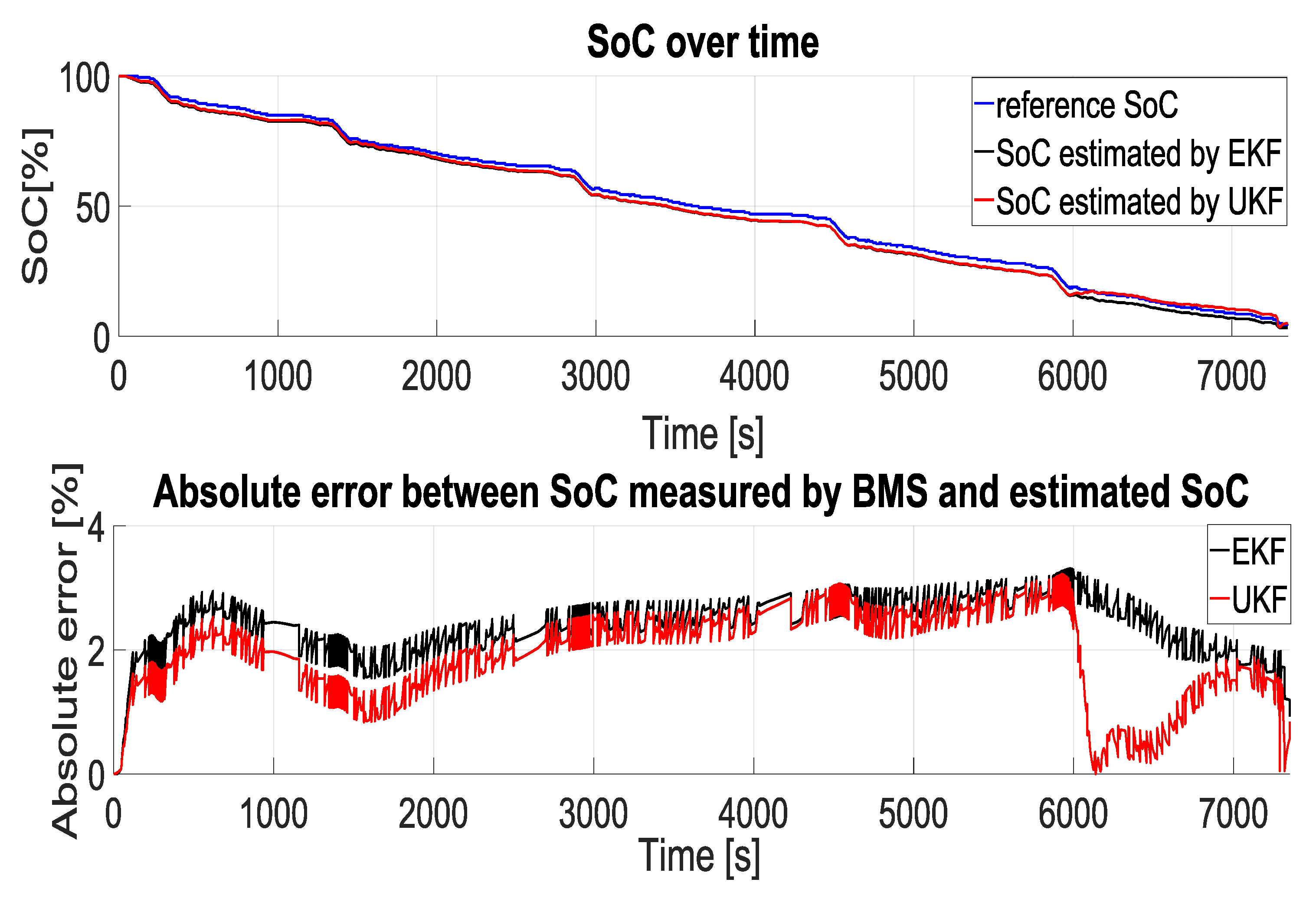
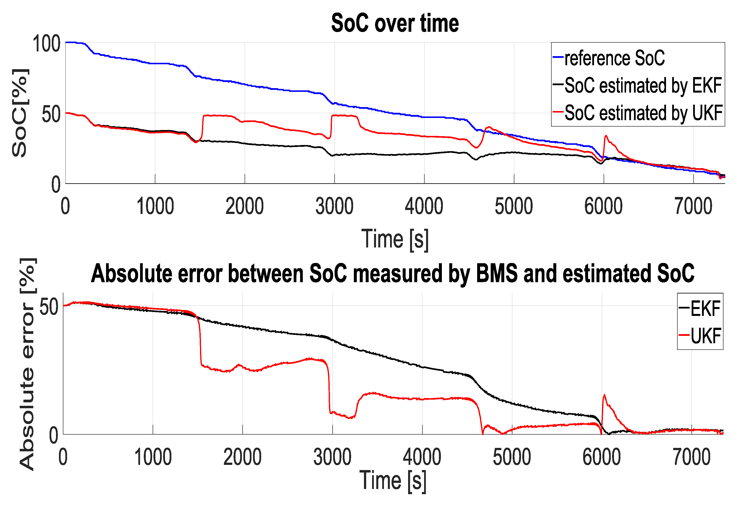
3.4. Results and Discussion

Using different resistance and capacitance values for the battery impedance presented in Table 2, the battery SoC is estimated during the HWFET and UDDS. Figure 9 provides the comparison of SoC estimation using EKF and UKF on a UDDS using the impedance model estimated on UDDS.

Figure 9 shows the high capability of the EKF and UKF to estimate the battery SoC precisely when there is no error for initial SoC. The SoC estimated by UKF is slightly better than the SoC estimated by EKF. Both estimation errors are always inferior to 4%. The reference SoC quantization causes the high-frequency oscillation of the absolute error. In fact, the SoC provide by the BMS has a precision of 0.5%.

Moreover, EKF and UKF provides robustness to the SoC estimation, even if the initial SoC is greatly different from the truth, and the estimated SoC converges to the reference value over time. Figure 10 shows this ability with an initial SoC error of 50%. Moreover, Figure 10 shows that the SoC estimation converges faster to the reference SoC when using UKF than EKF.

With the same parameters for EKF and UKF, similar conclusions are obtained when selecting the impedance model estimated on HWFET or both impedance models on the HWFET drive cycle.

The accuracy and robustness of the SoC estimation through an EKF or UKF can be adjust through two parameters: the measurement and model covariance noise. Those parameters symbolize, respectively, the confidence in the voltage measurement and the state equation that computes SoC. By selecting a high confidence in the measurement, the robustness is boosted at the cost of SoC estimation precision and vice versa. By choosing a high confidence in the model, the SoC estimation precision is increased, but the robustness is decreased and vice versa.

4. Conclusions

The main contribution of this manuscript is the development of a more robust and accurate mathematical battery impedance model capable of updating its impedance over the battery lifetime by using a passive impedance estimation approach. Compared to the original idea presented in the published conference paper [61], this manuscript explains, in detail, the previously developed method of transforming the battery impedance from a frequency domain to a time domain. This battery impedance estimation is validated by obtaining similar results for the same battery with different passive voltage and current profile. Furthermore, using those estimated impedances, accurate and robust battery SoC estimations through Kalman filters are achieved. In the original contribution of the published conference paper [19], only an EKF was applied. However, in this manuscript, the contribution has been extended by using an EKF and UKF, and comparing their performance regarding battery SoC estimation. Results show that the error between SoC estimated through EKF or UKF and SoC measured by the battery management system is less than 4%. Moreover, SoC estimated through EKF and UKF can converge to an accurate SoC even if the initial SoC error is large (50%). Furthermore, unlike paper [61], this manuscript shows that SoC estimation through UKF is more accurate and converges faster to the reference value than SoC estimated through EKF. Finally, those results are reproducible using both estimated impedance on both drive cycles.

5. Future Work

More meticulous tests, in which temperature would be kept constant, could be completed. A detailed comparison between the results of those experiments and an EIS might be mandatory to justify the precision of the new battery impedance estimation method. Furthermore, testing this methodology on a different battery chemistry needs to be done to prove that this method can be adapted to different battery technologies.

References

1. Wakihara, M.; Yamamoto, O. Lithium Ion Batteries: Fundamentals and Performance; Wiley-VCH: New York, NY, USA, 1998. [Google Scholar]
2. Matsuki, K.; Ozawa, K. General Concepts. In Lithium Ion Rechargeable Batteries: Materials, Technology, and New Applications; Ozawa, K., Ed.; Wiley-VCH: Weinheim, Germany, 2010. [Google Scholar]
3. Andrea, D. Battery Management Systems for Large Lithium-Ion Battery Packs; Artech House: Boston, MA, USA, 2010. [Google Scholar]
4. Panchal, S.; Khasow, R.; Dincer, I.; Agelin-Chaab, M.; Fraser, R.; Fowler, M. Numerical modeling and experimental investigation of a prismatic battery subjected to water cooling. Numer. Heat Transf. Appl. 2017, 71, 626–637. [Google Scholar] [CrossRef]
5. Panchal, S. Impact of Vehicle Charge and Discharge Cycles on the Thermal Characteristics of Lithium-Ion Batteries. Master’s Thesis, University of Waterloo, Waterloo, ON, Canada, 2014. [Google Scholar]
6. Coleman, M.; Lee, C.K.; Zhu, C.; Hurley, W. State of charge determination from EMF voltage estimation: Using impedance, terminal voltage, and current for lead-acid and lithium-ion batterie. IEEE Trans. Ind. Electron. 2007, 54, 2550–2557. [Google Scholar] [CrossRef]
7. Howey, D.; Yufit, V.; Mitcheson, G.; Offer, G.; Brandon, N. Impedance measurement for advanced battery management system. In Proceedings of the EVS International Battery, Hybrid and Fuel Cell Vehicle Symposium, Barcelona, Spain, 17–20 November 2013; pp. 1–7. [Google Scholar]
8. Zhu, J.; Sun, Z.; Wei, X.; Dai, H. A new lithium battery internal temperature in-line estimate based on electrochemical impedance spectroscopy measurement. J. Power Sources 2015, 274, 990–1004. [Google Scholar] [CrossRef]
9. Richardson, R.; Ireland, P.; Howey, D. Battery internal temperature estimation by combined impedance and surface temperature measurement. J. Power Sources 2014, 265, 254–261. [Google Scholar] [CrossRef]
10. Schmidt, J.-P.; Arnold, S.; Loges, A.; Werner, D.; Wetzel, T.; Ivers-Tiffe, E. Measurement of the internal temperature via impedance: Evaluation and application of a new method. J. Power Sources 2013, 243, 110–117. [Google Scholar] [CrossRef]
11. Bundy, K.; Karlsson, M.; Lindbergh, G.; Lundqviste, A. An electrochemical impedance spectroscopy method for prediction of the state of charge of a nickel metal hybride battery at open circuit and during discharge. J. Power Sources 1998, 72, 118–125. [Google Scholar] [CrossRef]
12. Rodrigues, S.; Munichandraiah, N.; Shukla, A. A review of state of charge indication of batteries by means of a.c. impedance measurements. J. Power Sources 2000, 87, 12–20. [Google Scholar] [CrossRef]
13. Blankem, H.; Bohlen, O.; Buller, S.; Doncker, R.; Fricke, B.; Hammounche, A.; Linzen, D.; Thele, M.; Sauer, D. Impedance measurements on lead acid batteries for state of charge and state of health and cranking capability prognosis in electric and hybrid electrical vehicles. J. Power Sources 2005, 144, 418–425. [Google Scholar] [CrossRef]
14. Troltzsch, U.; Kanoun, O.; Trankler, H. Characterizing aging effects of lithium batteries by impedance spectroscopy. Electrochim. Acta 2006, 51, 1664–1672. [Google Scholar] [CrossRef]
15. Barsoukov, E.; Macdonald, J.R. Impedance Spectroscopy: Theory, Experiment, and Applications; Wiley: Hoboken, NJ, USA, 2005. [Google Scholar]
16. Orazem, M.; Tribolle, B. Electrochemical Impedance Spectroscopy; Prentice Hall: Upper Saddle River, NJ, USA, 2011. [Google Scholar]
17. Ljung, L. System Identification: Theory for the User; Prentice Hall: Upper Saddle River, NJ, USA, 1999. [Google Scholar]
18. Jiangwei, L.; Mazzola, M.S. Accurate battery pack modeling for automotive applications. J. Power Sources 2013, 237, 215–228. [Google Scholar]
19. Hélène, P.; Granjon, P.; Guillet, N.; Cattin, V. Tracking of electrochemical impedance of batteries. J. Power Sources 2016, 312, 60–69. [Google Scholar]
20. Piret, H.; Sockeel, N.; Heiries, V.; Michel, P.H.; Ranieri, M.; Cattin, V.; Guillet, N.; Granjon, P. Passive and active tracking of electrochemical impedance of a drone battery. In Proceedings of the EEVC European Battery, Hybrid and Fuel Cell Electric Vehicle Congress, Brussels, Belgium, 1–4 December 2015. [Google Scholar]
21. Sockeel, N.; Ball, J.; Shahverdi, M.; Mazzola, M. Passive tracking of the electrochemical impedance of a hybrid electric vehicle battery and state of charge estimation through an extended Kalman filter. In Proceedings of the IEEE Transportation Electrification Conference and Expo (ITEC), Chicago, IL, USA, 22–24 June 2017. [Google Scholar]
22. Eberke, U.; Helmolt, R.V. Sustainable transportation based on electric vehicle concepts: A brief overview. Energy Environ. Sci. 2010, 3, 689–699. [Google Scholar] [CrossRef]
23. Acello, R. Getting into gear with the vehicle of the future. San Diego Bus. J. 1997, 18, 15. [Google Scholar]
24. Mitsubishi Motors. Specifications. Available online: https://www.mitsubishi-motors.com/en/showroom/i-miev/specifications (accessed on 6 October 2018).
25. Tesla. Tesla Model S. Available online: https://www.tesla.com/models (accessed on 6 October 2018).
26. Xiong, R.; Cao, J.; Yu, Q.; He, H.; Sun, F. Critical Review on the Battery State of Charge Estimation Methods for Electric Vehicles. IEEE Battery Enrgy Storage Manag. Syst. 2017, 6, 1832–1843. [Google Scholar] [CrossRef]
27. Ng, K.S.; Moo, C.S.; Chen, Y.P.; Hsieh, Y.C. Enhanced coulomb counting method for estimating state-of-charge and state-of-health of lithium-ion batteries. Appl. Energy 2009, 86, 1506–1511. [Google Scholar] [CrossRef]
28. Yan, J.; Xu, G.; Qian, H.; Xu, Y. Robust state of charge estimation for hybrid electric vehicles: Framework and algorithms. Energies 2010, 3, 1654–1672. [Google Scholar] [CrossRef]
29. Pop, V.; Bergveld, H.J.; Notten, P.H.L.; Regtien, P.P.L. State of the art of battery state of charge determination. Meas. Sci. Technol. 2005, 16, 93–110. [Google Scholar] [CrossRef]
30. Kozlowski, J.D. Electrochemical cell prognostics using online impedance measurements and model-based data fusion techniques. In Proceedings of the IEEE Aerospace Conference, Proceeding, Big Sky, MT, USA, 8–15 March 2003. [Google Scholar]
31. Shen, W.X.; Chan, C.C.; Lo, E.W.C.; Chau, K.T. A new battery available capacity indicator for electric vehicles using neural network. Energy Convers. Manag. 2002, 43, 817–826. [Google Scholar] [CrossRef]
32. Li, I.H.; Wei-Yen, W.; Shin-Feng, S.; Yuang-Shung, L. A merged fuzzy neural network and its applications in battery state of charge estimation. IEEE Trans. Energy Convers. 2007, 22, 697–708. [Google Scholar] [CrossRef]
33. Lee, Y.S.; Wang, W.Y.; Kuo, T.Y. Soft computing for battery state of charge (BSOC) estimation in battery string systems. IEEE Trans. Ind. Electr. 2008, 55, 229–239. [Google Scholar] [CrossRef]
34. Cheng, B.; Bai, Z.; Cao, B. State of charge estimation based on evolutionary neural network. Energy Convers. Manag. 2008, 49, 2788–2794. [Google Scholar]
35. Weigert, T.; Tian, Q.; Lian, K. State of charge prediction of batteries and battery-supercapacitor hybrids using artificial neural networks. J. Power Sources 2011, 196, 4061–4066. [Google Scholar] [CrossRef]
36. Hansen, T.; Wang, C.J. Support vector based battery state of charge estimator. J. Power Sources 2005, 141, 351–358. [Google Scholar] [CrossRef]
37. Shi, Q.; Zhang, C.; Cui, N. Estimation of battery state of charge using v-support vector regression algorithm. Int. J. Autom. Technol. 2008, 9, 759–764. [Google Scholar] [CrossRef]
38. Pattipati, B.; Sankavaram, C.; Pattipati, K.R. System identification and estimation framework for pivotal automotive battery management system characteristics. IEEE Trans. Syst. Man Cybern. C Appl. Rev. 2011, 41, 869–884. [Google Scholar] [CrossRef]
39. Lotfi, N.; Landers, R.G.; Li, J.; Park, J. Reduced-order electrochemical model-based SoC observer with output model uncertainty estimation. IEEE Transm. Control Syst. Technol. 2017, 25, 1217–1230. [Google Scholar] [CrossRef]
40. Satadru, D.; Ayalew, B.; Pisu, P. Nonlinear robust observers for state-of-charge estimation of lithium-ion cells based on a reduced electrochemical model. IEEE Trans. Control Syst. Technol. 2015, 23, 1935–1942. [Google Scholar]
41. Fang, H.; Wang, Y.; Sahinoglu, Z.; Wada, T.; Hara, S. State of charge estimation for lithium-ion batteries: An adaptive approach. Control Eng. Pract. 2014, 25, 45–54. [Google Scholar] [CrossRef]
42. Plett, G.L. Extended Kalman filtering for battery management systems of lipb-based hev battery packs: Part 1. Background. J. Power Sources 2004, 134, 252–261. [Google Scholar] [CrossRef]
43. Plett, G.L. Extended Kalman filtering for battery management systems of lipb-based hev battery packs: Part 2. Modeling and identification. J. Power Sources 2004, 134, 262–276. [Google Scholar] [CrossRef]
44. Plett, G.L. Extended Kalman filtering for battery management systems of lipb-based hev battery packs: Part 3. State and parameter estimation. J. Power Sources 2004, 134, 277–292. [Google Scholar] [CrossRef]
45. Lee, J.; Nam, O.; Cho, B.H. li-ion battery SOC estimation method based on the reduced order extended Kalman filtering. J. Power Sources 2007, 174, 9–15. [Google Scholar] [CrossRef]
46. Hu, C.; Youn, B.D.; Chung, J. A multiscale framework with extended Kalman filter for lithium-ion battery SOC and capacity estimation. Appl. Energy 2012, 92, 694–704. [Google Scholar] [CrossRef]
47. He, H.; Xiong, R.; Zhang, X.; Sun, F.; Fan, J. State of charge estimation of the lithium-ion battery using an adaptive extended kalman filter based on an improved thevenin model. IEEE Trans. Veh. Technol. 2011, 60, 1461–1469. [Google Scholar]
48. Chen, C.; Zhang, B.; Vachtsevanos, G.; Orchard, M.M. Machine condition prediction based on adaptive neuro-fuzzy and high-order particle filtering. IEEE Trans. Ind. Electr. 2011, 58, 4353–4364. [Google Scholar] [CrossRef]
49. Chen, C.; Vachtsevanos, G.; Orchard, M. Machine remaining useful life prediction based on adaptive neuro-fuzzy and high-order particle filter. In Proceedings of the PHM Society Annual Conference of the Prognostics and Health Management Society, Portland, OR, USA, 10–16 October 2010. [Google Scholar]
50. He, W.; Williard, N.; Osterman, M.; Pecht, M. Prognostics of lithium-ion batteries based on Dempster-Shafer theory and the Bayesian Monte Carlo method. J. Power Sources 2011, 196, 10314–10321. [Google Scholar] [CrossRef]
51. Wan, E.A.; van der Merwe, R. The unscented Kalman filter for nonlinear estimation. In Proceedings of the IEEE Adaptive Systems for Signal Processing Communications, and Control Symposium (AS-SPCC), Lake Louise, AB, Canada, 1–4 October 2000. [Google Scholar]
52. Julier, S.J.; Uhlmann, J.K.; Durrant-Whyte, H.F. A new approach for filtering nonlinear systems. In Proceedings of the IEEE American Control Conference (ACC), Seattle, WA, USA, 21–23 June 1995; Volume 3, pp. 1628–1632. [Google Scholar]
53. Julier, S.J.; Uhlmann, J.K. New extension of the kalman filter to nonlinear systems. In Proceedings of the SPIE Signal Processing, Sensor Fusion, and Target Recognition VI, Orlando, FL, USA, 21–24 April 1997; Volume 3068. [Google Scholar]
54. Pintelon, R.; Schoukens, J. System Identification: A Frequency Domain Approach; Wiley: Hoboken, NJ, USA, 2012. [Google Scholar]
55. Shin, K.; Hammond, J. Fundamentals of Signal Processing for Sound and Vibration Engineers; Wiley: Hoboken, NJ, USA, 2008. [Google Scholar]
56. Bendat, J.S.; Piersol, A.G. Random Data Analysis and Measurement Procedures, 4th ed.; Wiley: Hoboken, NJ, USA, 2010. [Google Scholar]
57. Mazzola, M.S.; Shahverdi, M. Li-Ion Battery Pack and Applications. In Rechargeable Batteries; Zhang, Z., Zhang, S.S., Eds.; Springer International Publishing: New York City, NY, USA, 2015; pp. 455–476. [Google Scholar]
58. Einhorn, M.; Conte, F.V.; Kral, C.; Fleig, J. Comparison, Selection, and Parametrization of Electrical Battery Models for Automotive Applications. IEEE Trans. Power Electr. 2013, 28, 1429–1437. [Google Scholar] [CrossRef]
59. He, H.; Xiong, R.; Fan, J. Evaluation of Lithium-Ion Battery Equivalent Circuit Model for State of Charge Estimation by an Experimental Approach. Energies 2011, 4, 582–598. [Google Scholar] [CrossRef]
60. MathWorks. Invfreqs. 2017. Available online: https://www.mathworks.com/help/signal/ref/invfreqs.html?searchHighlight=invfreqs&s_tid=doc_srchtitle (accessed on 12 October 2017).
61. MathWorks. Residue. 2017. Available online: https://www.mathworks.com/help/matlab/ref/residue.html?searchHighlight=residue&s_tid=doc_srchtitle (accessed on 12 October 2017).
62. Sockeel, N.; Shahverdi, M.; Mazzola, M.; Meadows, W. High-Fidelity Battery Model for Model Predictive Control Implemented into a Plug-In Hybrid Electric Vehicle. Batteries 2017, 3, 13. [Google Scholar] [CrossRef]
63. Sockeel, N.; Shi, J.; Shahverdi, M.; Mazzola, M. Sensitivity analysis of the battery model for model predictive control implemented into a plug-in hybrid electric vehicle. In Proceedings of the IEEE Transportation Electrification Conference and Expo (ITEC), Chicago, IL, USA, 22–24 June 2017. [Google Scholar]
64. Sockeel, N.; Shi, J.; Shahverdi, M.; Mazzola, M. Pareto front analysis of the objective function in model predictive based power management system of a plug-in hybrid electric vehicle. In Proceedings of the IEEE Transportation Electrification Conference and Expo (ITEC), Long Beach, CA, USA, 13–15 June 2018. [Google Scholar]
65. Sockeel, N.; Shi, J.; Shahverdi, M.; Mazzola, M. Sensitivity analysis of the vehicle model mass for model predictive based power management system of a plug-in hybrid electric vehicle. In Proceedings of the IEEE Transportation Electrification Conference and Expo (ITEC), Long Beach, CA, USA, 13–15 June 2018. [Google Scholar]
66. Shahverdi, M.; Mazzola, M.S.; Grice, Q.; Doude, M. Pareto Front of Energy Storage Size and Series HEV Fuel Economy Using Bandwidth-Based Control Strategy. IEEE Trans. Transp. Electrif. 2016, 2, 36–51. [Google Scholar] [CrossRef]
67. Shahverdi, M.; Mazzola, M.; Sockeel, N.; Gafford, J. High bandwidth energy storage devices for HEV/EV energy storage system. In Proceedings of the IEEE Transportation Electrification Conference and Expo (ITEC), Dearborn, MI, USA, 15–18 June 2014. [Google Scholar]
68. Shahverdi, M.; Mazzola, M.S.; Grice, Q.; Doude, M. Bandwidth-Based Control Strategy for a Series HEV with Light Energy Storage System. IEEE Trans. Veh. Technol. 2017, 66, 1040–1052. [Google Scholar] [CrossRef]
69. Zheng, Z.; Sun, J.; Liu, D. Online State of Charge EKF Estimation for LiFePO4 Battery Management Systems. In Proceedings of the IEEE International Symposium on Intelligent Signal Processing and Communication Systems (ISPACS), Tamsui, New Tapei City, Taiwan, 4–7 November 2012. [Google Scholar]
70. He, Z.; Gao, M.; Wang, C.; Wang, L.; Liu, Y. Adaptative State of Charge Estimation for Li-Ion Batteries Based on an Unscented Kalman Filter with an Enhanced Battery Model. Energies 2013, 6, 4134–4151. [Google Scholar] [CrossRef]
71. He, W.; Williard, N.; Chen, C.; Pecht, M. State of charge estimation for electric vehicles batteries using unscented kalman filtering. Microeletr. Reliab. 2013, 53, 840–847. [Google Scholar] [CrossRef]
72. Sun, F.; Hu, X.; Zou, Y.; Li, S. Adaptive unscented Kalman filtering for state of charge estimation of a lithium-ion battery for electric vehicles. Energy 2011, 36, 3531–3540. [Google Scholar] [CrossRef]
Figure 1. Frequency impedance estimation method.
Batteries 04 00052 g001
Figure 2.n-th” order impedance model of the battery.
Batteries 04 00052 g002
Figure 3. Picture of the Car of the Future Plug-in Series hybrid electric vehicle.
Batteries 04 00052 g003
Figure 4. Series PHEV block diagram of the Subaru BRZ 2015.
Batteries 04 00052 g004
Figure 5. Current and voltage profile and spectrogram during UDDS drive cycle.
Batteries 04 00052 g005
Figure 6. Coherence spectrogram for passive case during UDDS.
Batteries 04 00052 g006
Figure 7. Modulus Phase RMSE depending on the impedance battery model order “n”.
Batteries 04 00052 g007
Figure 8. Bode diagram of the estimated battery impedance.
Batteries 04 00052 g008
Figure 9. SoC estimated on UDDS drive cycle using impedance model estimated on UDDS with correct initial SoC.
Batteries 04 00052 g009
Figure 10. SoC estimated on UDDS drive cycle using impedance model estimated on UDDS with 46% initial SoC error.
Batteries 04 00052 g010