Application of Time-Resolved Multi-Sine Impedance Spectroscopy for Lithium-Ion Battery Characterization


1
Electrochemical Energy Conversion and Storage Systems Group, Institute for Power Electronics and Electrical Drives (ISEA), RWTH Aachen University, Jaegerstr. 17/19, 52066 Aachen, Germany
2
Jülich Aachen Research Alliance, JARA-Energy, Forschungszentrum Jülich GmbH, 52425 Jülich, Germany
3
Institute for Power Generation and Storage Systems (PGS), E.ON ERC, RWTH Aachen University, Mathieustraße 10, 52074 Aachen, Germany
4
Helmholtz Institute Münster (HI MS), IEK-12, Forschungszentrum Jülich GmbH, 52425 Jülich, Germany
*
Author to whom correspondence should be addressed.
Batteries 2018, 4(4), 64; https://doi.org/10.3390/batteries4040064
Submission received: 11 October 2018
/
Revised: 7 November 2018
/
Accepted: 12 November 2018
/
Published: 5 December 2018
Abstract
:Electrochemical Impedance Spectroscopy (EIS) is a valuable tool for the characterization of electrical, thermal and aging behavior of batteries. In this paper, an EIS measurement technique to acquire impedance spectra with high time resolution is examined, which can be used to gather impedance data during dynamic operating conditions. A theoretical analysis of the used multi-sine excitation signals is performed in detail and a practical measurement system is presented and validated. Afterwards, EIS measurements during the charging process of a lithium-ion battery are performed and discussed.
1. Introduction
In recent years, Electrochemical Impedance Spectroscopy (EIS) has proven to be a valuable tool for the characterization of electrical, thermal and aging behavior of battery cells and other electrochemical systems, such as supercapacitors [1]. Its results are widely used to parameterize battery models for state estimation in various applications [2]. While it has almost exclusively been used in a laboratory environment in the past, most recently there has been some progress to adapt and integrate EIS techniques into Battery Management System (BMS) for online monitoring of large battery systems [3,4,5], for example, as used in electric vehicles. This allows a much more precise online monitoring of the battery state, by being able to adapt models to the real aging behavior of the individual battery cells, or by monitoring the internal battery temperature with EIS measurements [6,7].
The working principle of the most commonly used form of Electrochemical Impedance Spectroscopy is to excite the battery with an electrical current of a defined frequency and to measure the voltage response (galvanostatic excitation). The acquired waveforms are then transformed into the frequency domain by means of the Discrete Fourier Transform (DFT). Dividing the complex frequency domain values of voltage and current at the excitation angular frequency allows calculation the impedance value of the battery cell for this frequency [8,9]:
By sequential excitation at different frequencies, a full impedance spectrum can be acquired. This spectrum defines the complex transfer function of the observed system (the battery cell). The underlying assumption of EIS is that the observed system can be treated as a causal, Linear Time-invariant (LTI) system. For batteries, this assumption is only valid under special circumstances. This somewhat limits the use of EIS if the battery cell is actively charged or discharged, as—depending on the measurement—the prerequisite of stationarity is not strictly fulfilled any more. By shortening the measurement time for a complete spectrum considerably, EIS could therefore be used under more operating conditions. This paper proposes a multisine impedance spectroscopy technique for lithium-ion batteries, which allows observation of the transient change of the impedance spectrum in real-time during operation of the battery cell. This enables the use of EIS for new purposes under “in-operando” conditions, for example, fault detection or measurement during various non-equilibrium operating conditions.
After deriving the necessary prerequisites for the acquisition of valid impedance spectra and their implications on the proposed method, the design of multi-sine excitation signals and the necessary measurement signal processing techniques is discussed. Afterwards, a practical measurement system is presented and validation tests are discussed in detail.
2. Usage of Multi-Sine Signals for Electrochemical Impedance Spectroscopy
Multi-sine signals have been used for impedance spectroscopy and transfer function measurements already for quite some time in different fields, like biomedical applications [10,11], material characterization [12] and also for battery measurements [8,13,14]. Barsoukov et al. [8] presented multi-sine measurements on NiMH battery cells, as well as half cell measurements on lithium ion cathode and anode materials for different levels of discharge. Schmidt [14] used a multi-sine EISmethod for acquiring impedance spectra in the region Hz to 1000 Hz during discharge operation to validate an impedance model of a lithium ion battery cell.
The general difference of multi-sine EIS compared to conventional stepped-sine, or also called “frequency sweep”, EIS lies in the fact that multiple frequencies can be excited in the same time by using multiple superimposed sine waves of different frequency. In the time domain, such a signal consisting of n frequency components can be described as:
The chosen values of amplitude , frequency and phase angle for each individual components, as well as the overall number N of frequency points, are the degrees of freedom when designing the excitation signal. Boundary conditions and design guidelines for these values for impedance spectroscopy on lithium-ion batteries are derived in subsequent chapters.
3. Prerequisites for Validity of Impedance Spectra
A basic requirement for the definition of a complex transfer function of the observed electrochemical system is that it fulfills the criteria of linearity, stationarity and causality [15]. For impedance spectroscopy, the practical meaning of linearity is that the amplitude and phase response of the system under test do not depend on the magnitude of the perturbation signal. Also, the system must not exhibit hysteresis in its response at [15]. For batteries, the nonlinear behavior due to diffusion and charge transfer effects means that this condition cannot be strictly fulfilled for any excitation signal. Barsoukov et al. [8] state that, at room temperature, a voltage magnitude response less than the thermal voltage of about 25 mV should be used. In practice, values of about 10 mV [8] for lithium-ion batteries, and even lower values down to 3 mV for lead acid batteries are used. For pure galvanostatic excitation, this means that the amplitude of excitation current has to be chosen before the measurement so that the voltage response stays within the chosen range. For single-sine EIS, this can be easily achieved either if the approximate impedance magnitude is known beforehand, or if the excitation amplitude can be controlled online during the measurement. For multi-sine excitation, it is not immediately obvious how to achieve a limited voltage response, as shown in the next chapter. Other requirements for valid impedance spectra are stationary and causal behavior of the test object or its transfer function, respectively. For battery cells, this practically implies that the internal state of the cell, be it temperature, state of charge or aging state, must not change significantly during the measurement (“steady-state” approximation). For example, special care has to be taken in regions of very high or low state of charge for lead-acid batteries, where depletion processes inside the cell can lead to large concentration gradients and therefore to rather large overpotentials [16]. Multi-sine EIS, due to its potentially faster measurement time, could therefore be advantageous in cases, where temporal changes in system behavior can be expected. However, plausibility checks of the acquired spectra have to be performed, for example, by utilizing the Kramers-Kronig relation [15] or the “Z-Hit” algorithm [17].
4. Design of Multi-Sine Excitation Signals
4.1. Frequency Distribution and Spacing
The goal of impedance spectroscopy measurements is to extract information about the frequency domain behavior of the battery under test and the underlying electrochemical and physical processes. However, information about the latter is not distributed equally over the resulting impedance spectrum: for lithium-ion batteries, the influence of the solid-electrolyte interphase, electrolyte- as well as solid-state diffusion and charge transfer processes behavior occur at different frequency ranges, which are partly overlapping each other [18]. Charge transfer and solid state diffusion takes place at both electrodes simultaneously, and therefore both electrodes contribute to the spectrum. Additionally, the shape of the spectra changes dramatically with temperature and state-of-charge (SoC) [19]. For stepped-sine EIS, given enough measurement time, a dense frequency grid can be measured sequentially. For multi-sine EIS, the maximum useful number of frequency points for a excitation signal is limited by the finite power of the overall signal, which is the sum of the power of the individual components of a signal with the base period .
The amplitude of the voltage response to each excitation signal component has to be large enough to be measurable with the finite accuracy of the used data acquisition system. This is especially important for online diagnosis, as the cell voltage measurement resolution of typical battery management systems is quite limited, usually to about 100–500 V. Therefore, only a relatively low number of frequency points should be used to reduce the resulting measurement errors due to quantization and other error sources. Choosing these points should be done with the goal to maximize the acquired spectral information. Sanchez et al. propose in [11] to choose a denser grid of frequency points in regions with high impedance dispersion, which equals to a high rate of impedance change over frequency. Alternatively, fixed distributions can be used. Typically, logarithmic distributions are used for impedance spectroscopy on batteries, as these achieve a better coverage of the spectrum than an equally spaced distribution with the same amount of frequency points. For multi-sine signals, second-order harmonic distortions due to the excitation of nonlinearities can be a problem. From this point of view, the chosen frequency points should optimally not be integer multiples of each other. However, if not all frequency points are integer multiples of the base frequency, spectral leakage can occur during windowing, as for a given window length incomplete periods of some frequency points are then included in the Fourier transformed signal. A working compromise can be to take special care that the excitation signal at the base frequency does not cause harmonic distortions, for example by proper scaling of the amplitude.
The useful lower limit for the frequency of a multi-sine signal depends on the condition under which the measurement is performed, as already derived in the last section. The upper limit also depends on the actual battery under test. At high frequencies, most types of batteries typically show some degree of inductive behavior, which depends on the geometric properties of the cell. For lithium-ion batteries, different type of cell formats exist, most importantly cylindric, pouch and prismatic cell types. While for small pouch cells, the impedance may not show inductive behavior for frequency ranges up to several , for cylindric or prismatic cell the capacitive electrochemical behavior at higher frequencies may be masked by the inductive influence of the jelly roll and current collector geometry [20]. However, impedance measurements at these frequencies may still be worthwhile, as the range of about [21] up to about [20,22] is linked to the solid electrolyte interphase (SEI) of the anode. At low temperatures, these features can be sufficiently pronounced in the spectra to be distinguished from the geometric influence [22].
Another constraint for measuring impedance at higher frequencies, especially in an on-board EIS system integrated into the BMS, is the achievable sampling rate and therefore analog bandwidth. While it is theoretically sufficient to fulfill the Nyquist-Shannon criterion to fully recover a signal from discrete sampling points, noise and non-ideal nature of analog filters typically lead to the necessity of some degree of oversampling. To reduce complexity and cost of the data acquisition system, Schmitz et al. [23] made an interesting proposal: As typically the exact frequency points are not of interest for impedance spectroscopy, undersampling can be utilized purposefully: by choosing the frequency distribution in a way that the resulting aliasing frequencies for the chosen, sub-Nyquist sampling rate are known and unique, the information from higher spectral components can be recovered by Fourier transformation of the signal at the aliasing frequencies.
However, this means that special care has to be taken that no high-frequency distortions, for example due to electromagnetic interference, distort the signal at the same aliasing frequencies. Therefore, sufficient band-pass filtering of the signal before quantization is still necessary.
For the spectral analysis of measured time domain signals, usually the Fast Fourier Transform (FFT) algorithm is used. The frequency resolution of the FFT is inversely proportional to the number of sampling points: For example, at a sampling rate of 6 kHz a sampling period of 100 ms results in acquired samples. The result of the FFT are spectral components. Each of these components, commonly called “bins”, holds information about a certain frequency range of , which results in a spectral resolution of in this example. To achieve a higher frequency resolution either a higher sampling rate or a longer sampling interval must be used. For impedance spectroscopy on batteries, a high frequency resolution is crucial because of the typically high number of excitation points at low frequencies below 10 Hz. However, combined with a high excitation signal bandwidth, and therefore high necessary sampling rate, this leads to a high number of needed sampling points for sufficient frequency resolution, which in turn limits the temporal resolution of the acquired spectra. This fundamental trade-off can only be resolved by using alternative techniques like Wavelet transforms [24], which make both a high time- and frequency-resolution possible.
4.2. Time-Domain Behavior: Amplitude Response Limitation and Crest Factor Optimization
As already stated above, it is required to limit the response amplitude during EIS to achieve linear operation of the battery under test. This can be achieved by appropriately choosing the amplitude of the excitation signal. The amplitude of each individual component of a multi-sine signal, as defined in Equation (2), could be chosen independently from the other components to achieve the desired voltage response magnitude for each frequency point. The amplitude could either be set before the start or be actively controlled during the measurement. The latter could be achieved in a similar way as described in [9] for single sine excitation. Given the magnitude of the Fourier transformed voltage response signal at frequency and comparing it to the desired response magnitude , a new excitation amplitude can be determined by using the calculated impedance value of the last measurement cycle:
However, solely choosing the amplitude values separately for each frequency component has the drawback of not being able to limit the voltage amplitude response to the overall multi-sine excitation signal. Depending on the initial phases of the excitation signal, the resulting amplitude response can be much larger than desired, or clipping could occur if the excitation circuit is not able to source the desired peak currents with changing output voltage.
Additionally, the resulting envelope curve of the multi-sine signal can be scaled, so that the following condition is fulfilled in each period of the lowest frequency component of the multi-sine signal:
denominates the moving average over one period, which, given that the excitation signal has a mean value of zero, equals the battery cells’ open circuit voltage (OCV) if the voltage response is linear. A scale factor applied to the overall excitation signal can be defined to fulfill Equation (5), which again can either be defined a priori or be tuned by a control-loop during the measurement:
This still leaves the possibility to choose the individual amplitudes to achieve a sufficient signal-to-noise ratio for each frequency if the impedance magnitude varies considerably over the observed frequency range.
Equation (7) offers another degree of freedom to shape the time domain form of the excitation signal: By changing the initial phase values of the individual components, the so called crest factor (CF) of the resulting signal can be influenced. This values describes the difference between the maximum and minimum amplitude value of the observed signal, divided by its root-mean-square (RMS) value [25]. This relationship can be expressed by the following equation:
As multi-sine signals are used in many different areas of applications besides impedance spectroscopy, and minimizing the crest factor limits the peak power value of the signal, there has been a significant number of publications which are proposing strategies for crest factor optimization. The exact theoretical solution, which consists in selecting the optimal starting phases of the frequency components, is still an unsolved mathematical problem, according to literature [26]. Therefore, the proposed strategies are either a simplified analytical description of the problem, or the use of nonlinear numerical optimization methods.
One of the first optimization strategies, besides just choosing random initial phase values, was proposed by Schroeder in [25]. By choosing the initial phase values of a flat-power spectrum signal according to the following equations, decent crest factor values can be achieved, at least for signals with a uniform distribution of frequency components:
where N denotes the number of frequency components and k is the integer harmonic with respect to the lowest frequency component. However for multi-sine signals with non-uniform frequency distribution, this strategy does not produce significantly better results than simple random choosing of the phase values [27]. More sophisticated methods, based on genetic optimization [28], parameter variation approaches [10] or other iterative algorithms [29,30] were also proposed.
To assess the influence of signal bandwidth together with the nonlinear distribution of frequency points on the achievable crest factor, three different synthetic multi-sine signals were generated and crest factor optimization for these signals was performed with different optimization strategies. The properties of these signals are shown in Table 1. Regarding frequency range and distribution, Signal A is a multi-sine signal with good properties for EIS measurements on batteries, with a frequency range from 1 Hz–1 kHz in 21 frequency points (7 per decade). These are distributed quasi-logarithmic, which means that unique integer values are chosen, whereas a pure logarithmic distribution would have multiple points in the range of 1 Hz to 2 Hz. Signal B has the same frequency range, but a linear distribution. Signal C is a high bandwidth signal with frequency points up to 1 MHz.
The analytically calculated values according to Schroeder, as defined in Equation (9), are used as initial phase values for the other optimization strategies. As can be noted in Figure 1, using these values on their own only gives acceptable results for the linear frequency distribution of Signal B. For further optimization, three different generic nonlinear optimization methods and one specific CF optimization strategies were tested: The considered generic methods are the pattern search algorithm patternsearch [31], the downhill simplex algorithm fmincon and the genetic optimization algorithm implementations of MATLAB R2015a. In addition, the algorithm proposed by Yang et al. [29] was implemented, which is based on the concept presented by van der Ouderaa et al. [32]. The working principle is as following:
- Step 1: Synthesize signal in frequency domain with initial phase values.
- Step 2: Transfer into time domain by inverse FFT.
- Step 3: Clip signal peaks according to a specified criterion.
- Step 4: Transfer into frequency domain by FFT.
- Step 5: Save phase new values for desired frequency components.
- Step 6: Repeat with new phase values.
The clipping in the time domain introduces additional harmonics in the frequency domain, which are disregarded in the further analysis, as only the frequency components of the original signal are used further. While it was initially proposed to use a fixed clipping value [32], Yang et al. proposed a logarithmic clip function based on the iteration index [29]. As the results in Figure 1 show, this algorithm has generally a slightly performance in comparison to the generic optimization strategies for the signals A and B. For Signal C, with its significantly higher bandwidth, it results in a notably worse CF value. The generic optimization methods yield quite similar results, with the genetic optimization strategy performing slightly better than downhill simplex and pattern search.
Generally it is noticeable that Signal B, with its linear frequency distribution can be optimized to significantly lower CF values compared to signals with (quasi-)logarithmic distribution. This is in accordance with the observations in [10]. The reason for this behavior are likely the strongly differing power density spectra of linear and logarithmic distribution, and especially the latter having a nonuniform frequency spacing. The time domain waveforms of the optimized signals A and B in Figure 2 also indicate the differences, with the logarithmic frequency distribution of Signal A having a much more irregular waveform. It can therefore be concluded that, due to the inherently higher CF of logarithmic spaced signals, special care has to be taken during EIS measurements to achieve proper signal scaling and to verify the operation under LTI assumptions.
5. Signal Processing—Frequency Domain Transformation and Windowing
After presenting design constraints of multi-sine excitation signals, this chapter briefly discusses the necessary steps for signal processing and subsequent analysis of the acquired impedance spectra. The basic principle of the proposed time-resolved EIS measurement technique lies in the periodic repetition of the multi-sine excitation in combination with a sliding-window discrete Fourier-transform (DFT). The achievable time resolution for a full spectrum is dependent on the lowest frequency component of the excitation current, as a full signal period is needed for a DFT coefficient calculation. If the lowest frequency is 1 Hz, the minimum time resolution therefore is . However, as only one period is used, the result for this lowest frequency component becomes susceptible to jitter, noise phenomena and DC offsets of the signal acquisition system, which leads to a higher variance of the measured impedance.
This issues also exists with the traditional, stepped-sine excitation. Therefore, for stepped-sine EIS measurements, the DFT is typically performed over multiple periods of the excitation signal. A similar approach can be used for multi-sine EIS as well: by using a sliding DFT window of an integer multiple size of a new DFT value can be calculated every , while using n lowest frequency periods to lower the influence of noise. Figure 3 illustrates this principle. In this example, a Hann window is multiplied with the time domain signal, which lowers the influence of leakage effects caused by the fact that the first and last sampled value may not be exactly at zero crossing of the fundamental frequency component. The effect of the sliding window technique can be evaluated by observing the standard deviation of acquired impedance values: In Figure 4, the standard deviation of 3600 consecutively measured absolute impedance values of a reference impedance device is plotted over frequency in the range of 1 Hz to 1 kHz. The exact measurement setup is explained in detail in Section 6.3. It can be seen that by expanding the window length to 3 s the standard deviation for lower frequency components can be lowered considerably, especially if also a Hann window is used. The drawback of longer window lengths is a lowered sensitivity to very fast signal changes due to the “moving-average” like effect of the longer window sizes and non-unity weight values of the Hann window. However this is not an issue in most applications, as impedance changes gradually over time with changing SoC and temperature.
Using a continuous excitation has the additional benefit of not having to deal with settling behavior effects during most of the measurement. If the excitation current signal would only be switched on for a single base period of , settling effects would lead to significant distortion at the lower frequencies of the measured voltage response. However if the signal is repeated continuously, the steady-state response can be measured accurately after waiting for one to two periods of the base frequency at the beginning of measurement. For single-sine or stepped-sine excitation, the first periods therefore cannot be used, which further prolongs the time for acquiring a single impedance measurement point [33].
6. Experimental Comparison of Stepped-Sine and Multi-Sine Excitation
6.1. Measurement Setup
To evaluate performance of the proposed multi-sine, time-resolved EIS measurement scheme, measurements on two different reference impedances are performed. As measurement system, a modified version of the Digatron EISmeter was used. This EIS measurement system was originally developed at the authors’ institute and is now commercially distributed by the company Digatron. The EISmeter is specifically designed to measure the small impedance of battery cells in laboratory test setups. It features an AC current amplifier with a peak output of at frequencies up to 6 kHz, and a 24-bit analog-to-digital conversion for current and voltage measurement at a sample rate of 96 kSPS. EIS measurements with this device are normally performed with a stepped-sine excitation, which consecutively measures different frequencies. All necessary signal processing calculations are performed in the included FPGA. In this work, a modified version is used which allows to directly specify arbitrary waveforms for the excitation current. This is achieved by the addition of an Ethernet interface. With a connected host PC, current values can be set and raw measurement values of voltage and current can be read back in real-time. All digital signal processing is therefore done on the host PC using MATLAB R2015a. The measurement setup is shown in Figure 5. All experiments are performed in a temperature controlled chamber (not shown).
6.2. EIS Measurements of Precision Shunt Resistor
To assess the quality of the multi-sine excitation in comparison with traditional stepped-sine excitation, using real batteries is not optimal: subtle changes in temperature lead to a comparatively high change of impedance for most batteries. Additionally, the measurement results would be virtually impossible to reproduce, as a battery with the exact aging state would be needed. Therefore, a precision coaxial low-inductance shunt resistor (HILO ISM 5P/10) with a nominal resistance of 10 m and a temperature coefficient of 50 ppm/K is used for testing purposes. These (or similar) devices are commonly used for calibration of EIS measurement devices in laboratory setups. As excitation signal, a stepped-sine and a multi-sine signal are compared in a continuous measurement of 3600 s length in galvanostatic mode. The measurement is conducted with identical devices and cabling setup, inside a temperature controlled chamber at 25 C ambient temperature. No prior instrument calibration is performed. The properties of the two signals are shown in Table 2. While frequency range and spacing are identical, the number of periods per frequency point is different, and variable for the multi-sine signal. For the stepped sine signal, 10 periods per frequency point are used, with a minimum measurement duration of 1 s. Including pauses of about 1 s between points, this sums up to about 60 s of measurement time for one spectrum. The number of impedance points generated during 3600 s overall measurement time is therefore about 60 times as high when using the multi-sine signal. The signals have been designed to be representative of typical use cases. While it is theoretically possible to scale the signals to have identical RMS values (or identical peak values—but not both at the same time), this leads to suboptimal results for either multi-sine or stepped-sine in real applications.
In this example, the peak current amplitude of the overall multi-sine signal is about 3.5 times higher than for the stepped-sine, although on a per-frequency component base, the components of the multi-sine signal have only an amplitude of about mA, which is about 40% of the stepped-sine amplitude. Consequently, the signal power of the multi-sine signal is nearly six times higher. However, the multi-sine signal energy is more than 10 times smaller per acquired spectrum, which can be advantageous for the application.
In Figure 6 results of the measurement are shown. Multi-sine and single-sine excitation generally show very good conformance. The multi-sine measurements show a relative deviation from the single-sine values of much lower than 0.5% for the magnitude . For the phase, the relative deviation is higher for low frequencies, which is mostly due to the extremely low phase shift of less than of the shunt resistor at low frequencies (which should ideally be zero). The standard deviation of both measurement techniques is generally below 25 for the magnitude, with the exception of the 495 Hz and 704 Hz point in the single-sine measurement. These points also show a significantly higher standard deviation. In the multi-sine measurement also a small offset is noticeable for these frequency points. The origin of these deviations is possibly related to measurement noise of the EISmeter: In [33], Baumhöfer analyzed the noise power spectral density (PSD) of current and voltage measurement of the device. Different low-level peaks exist in the spectrum, some very near in frequency to the values at about 495 Hz (near 10th harmonic of grid frequency) and 704 Hz, which show the highest deviations in the performed measurement. However because of their rather low level, the impact on measurement results is quite limited. Also, at least the difference in mean value can easily be removed by instrument calibration.
6.3. EIS Measurements of Reference Impedance Device
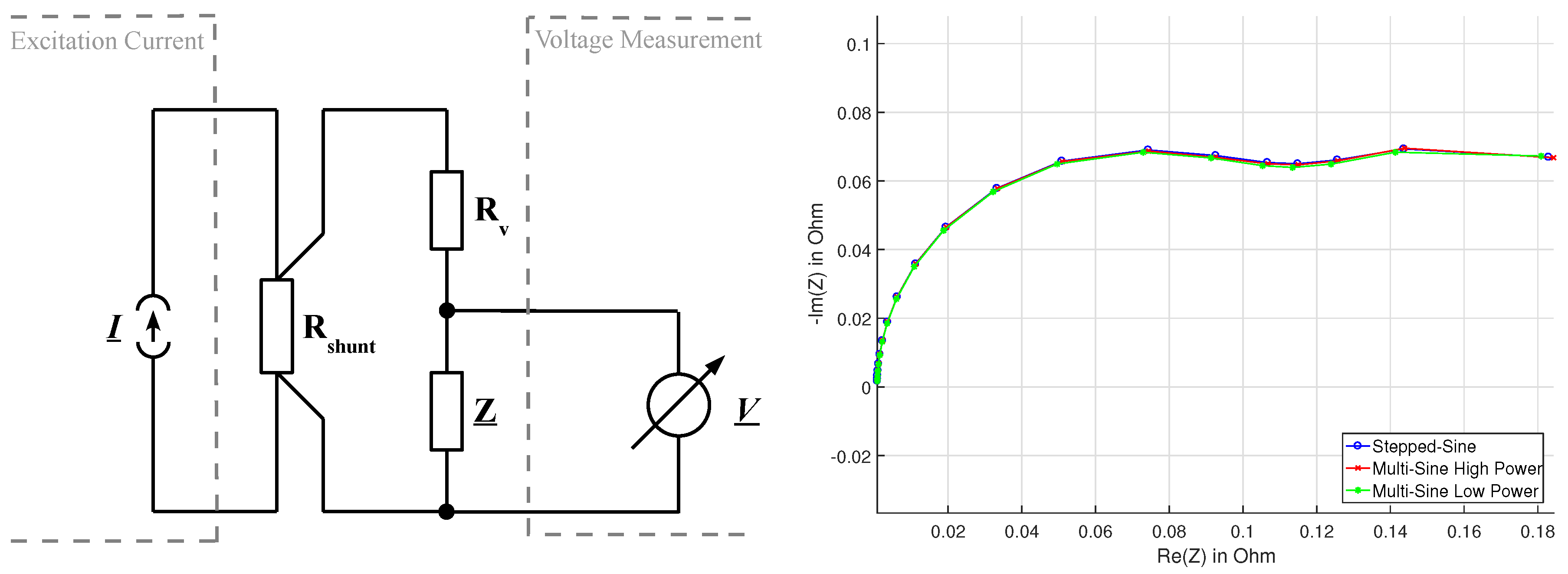
To further evaluate the quality of the measurement results with multi-sine EIS, another device under test is used: an artificial reference impedance device, which is designed to approximate more closely the impedance behavior of the real battery cell was developed at the authors’ institute several years ago [34]. It consists of discrete resistors and ceramic capacitors and is used for the relative comparison of results from different EIS acquisition devices under identical measurement conditions. The schematic is depicted in Figure 7 left. Compared to the coaxial shunt resistor, the reference impedance has a strong frequency dependent behavior of impedance magnitude and phase. However, as ceramic capacitors show a voltage dependent capacitance behavior, deviations can be expected if vastly different measurement conditions are used. Also considering statistical deviations in component values, an absolute comparison of measurement results to theoretical calculated values does only give very limited insight, and is therefore omitted here.
For this test, the identical stepped-sine measurement signal was used. The multi-sine signal was scaled to two different magnitudes. A full overview is given in Table A1 in the Appendix A. The first multi-sine signal used for this test, referred to as “Multi-Sine High Power”, is identical to the signal used in the test on the precision shunt resistor in Section 6.2. The second signal is a reduced amplitude version, referred to as “Multi-Sine Low Power”. The peak current amplitude of this signal was scaled down to about 26% of the high power signal, and is now close to the single-sine amplitude value. This leads to a reduction in signal power of 93% to W—Compared to W for the stepped sine. The total signal energy of the low-power multi-sine signal is only about 0.6% of the stepped-sine signal energy value.
The measurement results on the reference impedance device are shown in Figure 7 (right). The two excitation methods show again very similar results. Although, deviations for Re(Z) and Im(Z) are clearly visible for the low-power multi-sine. Detailed results are shown in Figure A1 in the Appendix A. These figures show that, compared to the stepped-sine signal, the difference in magnitude is below 2.5% for the low power signal, and below 1% for the high power signal. The standard deviation for low frequencies is significantly higher for both cases of the multi-sine signal. Most likely, the lower number of considered periods for frequencies below 10 Hz in the multi-sine measurement leads to higher influence of 1/f noise for these data points. Regarding the phase values, compared to stepped sine the deviation from mean value for both multi-sine measurements is similar, and only slightly better for the high power signal. The standard deviation also shows peaks at higher frequencies above 200 Hz, as was already seen in the shunt measurement.
In summary, the low power multi-sine signal still produces usable results for many applications, and does not show a significantly higher standard distribution compared to the high power signal. The difference in mean value however should be taken into account, but could, in theory, be corrected by proper calibration.
7. Application of Time-Resolved EIS for Lithium-Ion Battery Characterization
In this section, an exemplary application scenario for the proposed time-resolved EIS measurement technique is laid out and measurements on a lithium-ion battery cell are presented. The application of fast EIS measurements is most useful during conditions of changing ambient or internal states, for example during charging or discharging, or changing temperature for thermal characterization. In laboratory setups, this can save significant amounts of time during characterization measurements.
As an example, EIS measurements during a C constant-current/constant-voltage charge procedure on a Ah NMC/graphite lithium-ion pouch cell (Kokam SLPB526495) are conducted. The charge process is temperature-controlled by placing the cell inside a temperature chamber at 15 C ambient temperature and application of a heating foil to the cell. A temperature sensor (Maxim DS18B20) is placed on the cell surface on the opposite site of the heating foil. The setup is shown in the left part of Figure 8.
During operation, the cell surface temperature is regulated to 20 C by a PID controller running on a microcontroller and PWM control of the heating foil current. The resulting temperature behavior during charging is shown in the right part of Figure 8. While this setup enforces a certain temperature gradient through the cell, as heater and sensor are on opposite sides of the battery, this has the advantage to keep the temperature distribution nearly constant during charging, apart from a short period of time right at begin of charging, where some undershoot is visible. In contrast, without temperature control, the cell temperature has a greater variation due to varying heat generation inside the cell and cooling by free convection. Consequently, this makes it possible to observe the cell impedance in dependence of the state-of-charge and not the temperature.
The EIS measurements are performed with a similar signal as in Section 6.2, with a frequency range of 1 Hz to 1 kHz. For the tested cell, this allows to assess the behavior of what is most likely the charge transfer semicircle, as is visible in the Nyquist plot in Figure 9c. In the high frequency range, this cell shows a very low inductance, as—in contrast to many larger prismatic cells and also cylindric cells—the crossover frequency from the capacitive to inductive behavior is above 1 kHz. However this makes sense, given that the cell is relatively small, is made of stacked electrode foils, and has no long, narrow current collectors, which overall results in a low-inductance geometrical shape.
To assess the compliance to LTI criteria, the Kramers-Kronig relations [36] can be used. These transformations describe the relation between the imaginary part and the real part of an impedance spectra of a linear, time-invariant, causal system. To achieve a robust validation, the Lin-KK software tool, developed by Karlsruhe Institute of Technology, is used [35,36,37,38]. This tool performs a fitting procedure using multiple RC-elements and outputs the residuals between fit and measurement, which should ideally be smaller than about 0.5% for a valid measurement under LTI conditions [35]. For the presented measurement during charge conditions this is the case, as can be seen in the bottom part (d) and (e) of Figure 9, where two exemplary residuals for two measured spectra shortly after beginning and before end of charge are plotted. This also shows that the correction of the DC voltage drift works correctly.
The acquired, instantaneous values of real and imaginary part of the small-signal impedance are plotted separately in Figure 9a,b versus the absolute state of charge. To provide an overview of the change in a more common form of graphical representation, also a Nyquist plot of the first and last acquired spectra is shown. The trend for Re(Z) and Im(Z) is somewhat surprising, as it does not show a pure linear or exponential behavior versus charge. Instead, a distinct plateau and inflection point is visible for both in the lower third of the charge state. A second, significantly weaker inflection point can be seen at high state of charge, towards the end of the constant-current charging phase. Conventional, stepped-sine EIS measurements at discrete SoC points are not able to make this behavior observable. Most likely some sort of interpolation between points would be used between acquired spectra, as shown by Schiller et al. in [17]. This would likely smooth out the observed inflection points, except if a extremely dense SoC grid is chosen, which is unpractical due to the long measuring times.
The terminal voltage of the battery cell is also plotted in Figure 9 on a second y-axis. It can be seen that the described inflection points coincide with changes in the cell voltage slope behavior. This suggests that the results from EIS measurement can be correlated with results from differential voltage analysis (DVA). The DVA can, for example, be used to assess the aging mechanisms in battery cells. More details on this topic can be found e.g., in the publication by Lewerenz et al. [39].
To compare the results of EIS and DVA, the measured data of voltage as well as the real or imaginary part of the impedance must be fitted to an analytical function, to suppress noise which would distort the result if simple numerical differentiation would be used. In this case, a cubic smoothing spline function is used, which can be differentiated analytically. The result is shown in Figure 10 for Re(Z) and the DVA of the terminal voltage during the constant current phase of the charge process. A clear relation can be observed between change of slopes of voltage and real part of the small signal impedance value, as marked by the dashed lines. However, it has to be noted that due to the rather high charge current rate of C, the features of the DVA are likely not as pronounced as possible within lower current rate charge or discharge. For clarity, the slope change of Re(Z) starting at about Ah of stored charge is shown zoomed in, as it is significantly smaller than the changes at begin of charge. In the DVA, a change in slope behavior at this point is just barely visible. Also visible in the zoomed area is that the higher frequency parts of the spectrum (green-blue lines) show a different behavior.
The features seen in the DVA are likely the transitions between different intercalation stages of lithium into the graphitic anode of the cell. If this is the case, a plausible explanation for the correlation of the impedance change occuring at the same state-of-charge can be given: In [40], Takami et al. show through measurements on different treated graphites that the anodic polarization resistance of a graphite insertion electrode, consisting of the charge transfer resistance and SEI film resistance, is correlated with the degree of lithiation, and shows especially strong changes at phase transitions. However without further investigation it cannot be proven with absolute certainty that this is the exact effect seen in this measurement.
8. Conclusions and Outlook
This paper discussed theoretical considerations and practical design of multi-sine excitation signals for electrochemical impedance spectroscopy on battery cells. A practical measurement system for acquiring time-resolved EIS measurements was presented and validated through measurements on different artificial reference devices. The proposed method is able to acquire single impedance spectra in the range of 1 Hz to 1 kHz up to about 60 times faster during continuous measurement operation. However, the useful lower limit regarding the measurement frequency range is still determined by the rate of change of the battery state during dynamic operation conditions.
EIS Measurements on a lithium-ion cell during charging were performed, and the data was compared to results from differential voltage analysis. A clear connection between changes in small signal impedance and cell voltage slope could be shown. Future work should include a more detailed analysis of the connection of the data acquired from DVA and EIS. Tests under different charging and discharging conditions should be carried out, including measurements at low temperature. The change of these parameters during cyclic aging experiments should be observed and compared to each other.
Also, the developed measurement method can be used to acquire EIS spectra at abuse conditions, such as overcharging and high temperature operation to analyze the effects of these conditions to the small signal impedance of the battery, which will be shown in a future publication. Afterwards, these results can be used to design a onboard EIS system, which could significantly improve the online-diagnostic capabilities of battery management systems, to improve the safety and lifetime estimation of battery systems.
Author Contributions
Conceptualization, H.Z. and D.U.S.; Formal analysis, H.Z.; Investigation, H.Z.; Methodology, H.Z.; Software, F.R.; Validation, F.R.; Writing—original draft, H.Z.; Writing—review & editing, F.R. and D.U.S.
Funding
Parts of this research work were funded through the ZIM (“Zentrales Innovationsprogramm Mittelstand”) project Ausfallsichere Batterie (FKZ: KF3468301PR4) by the german Federal Ministry of Economic Affairs and Energy. The responsibility for this publication lies solely with the authors. The authors also acknowledge the continued funding of the Federal Ministry of Economic Affairs and Energy in the scope of the EXIST research transfer project sBat-safer Battery.
Acknowledgments
The authors also want to thank Thorsten Baumhöfer for the initial development of the modifications to the EISmeter, which are further used in this work.
Conflicts of Interest
The authors declare no conflict of interest.
Abbreviations
The following abbreviations are used in this manuscript:
| BMS | Battery Management System |
| DFT | Discrete Fourier Transform |
| EIS | Electrochemical Impedance Spectroscopy |
| FFT | Fast Fourier Transform |
| LTI | Linear Time-invariant |
Appendix A

Table A1.
Properties of evaluated excitation signals for reference impedance device measurement.
| Signal | Stepped-Sine | Multi-Sine High Power | Multi-Sine Low Power |
|---|---|---|---|
| 1 Hz | 1 Hz | 1 Hz | |
| 1 kHz | 1 kHz | 1 kHz | |
| Frequency Distribution | quasi-log. | quasi-log. | quasi-log. |
| Frequency Points | 20 | 20 | 20 |
| Periods per Point | 10 | variable | variable |
| RMS Current | mA | mA | mA |
| Amplitude per Frequency Point | mA | mA | mA |
| Peak Current Amplitude | mA | mA | mA |
| Crest Factor | 1.41 | 2.53 | 2.53 |
| Signal Power | W | 561 W | W |
| Signal Length | s | 1 s | 1 s |
| Signal Energy | mJ | mJ | mJ |
Pause intervals between frequency points excluded; Maximum of absolute value; At 10 m pure-ohmic load.
Figure A1.
Impedance measurement of reference impedance device. From (left) to (right): Comparison of mean values for multi- and stepped-sine, relative deviation for multi-sine, comparison of standard deviation. (Top row): Magnitude of Z. (Bottom row): Phase of Z.
Figure A1.
Impedance measurement of reference impedance device. From (left) to (right): Comparison of mean values for multi- and stepped-sine, relative deviation for multi-sine, comparison of standard deviation. (Top row): Magnitude of Z. (Bottom row): Phase of Z.

References
- Kurzweil, P.; Shamonin, M. State-of-Charge Monitoring by Impedance Spectroscopy during Long-Term Self-Discharge of Supercapacitors and Lithium-Ion Batteries. Batteries 2018, 4, 35. [Google Scholar] [CrossRef]
- Vyroubal, P.; Kazda, T. Equivalent circuit model parameters extraction for lithium ion batteries using electrochemical impedance spectroscopy. J. Energy Storage 2018, 15, 23–31. [Google Scholar] [CrossRef]
- Howey, D.A.; Mitcheson, P.D.; Yufit, V.; Offer, G.J.; Brandon, N.P. Online Measurement of Battery Impedance Using Motor Controller Excitation. IEEE Trans. Veh. Technol. 2014, 63, 2557–2566. [Google Scholar] [CrossRef]
- Ringbeck, F.; Nordmann, H.; Sauer, D.U. Design eines preiswerten Impedanzspektroskopiesystems für den Einsatz in Batteriepacks. In Tagungsband zum Power and Energy Student Summit 2014 in Stuttgart; Tenbohlen, S., Ellerbrock, A., Eds.; Univ.: Stuttgart, Germany, 2014. [Google Scholar]
- Din, E.; Schaef, C.; Moffat, K.; Stauth, J.T. Online spectroscopic diagnostics implemented in an efficient battery management system. In Proceedings of the 2015 IEEE 16th Workshop on Control and Modeling for Power Electronics (COMPEL), Vancouver, BC, Canada, 12–15 July 2015; IEEE: Piscataway, NJ, USA, 2015; pp. 1–7. [Google Scholar] [CrossRef]
- Srinivasan, R.; Carkhuff, B.G.; Butler, M.H.; Baisden, A.C. Instantaneous measurement of the internal temperature in lithium-ion rechargeable cells. Electrochim. Acta 2011, 56, 6198–6204. [Google Scholar] [CrossRef]
- Richardson, R.R.; Ireland, P.T.; Howey, D.A. Battery internal temperature estimation by combined impedance and surface temperature measurement. J. Power Sources 2014, 265, 254–261. [Google Scholar] [CrossRef]
- Barsoukov, E.; Macdonald, J.R. (Eds.) Impedance Spectroscopy: Theory, Experiment, and Applications, 2nd ed.; Wiley-Interscience a John Wiley & Sons Inc. Publication: Hoboken, NJ, USA, 2005. [Google Scholar] [CrossRef]
- Kiel, M. Impedanzspektroskopie an Batterien unter Besonderer Berücksichtigung von Batteriesensoren für den Feldeinsatz; Aachener Beiträge des ISEA; Shaker: Aachen, Germany, 2013; Volume 67. [Google Scholar]
- Ojarand, J.; Min, M.; Annus, P. Crest factor optimization of the multisine waveform for bioimpedance spectroscopy. Physiol. Meas. 2014, 35, 1019–1033. [Google Scholar] [CrossRef] [PubMed]
- Sanchez, B.; Vandersteen, G.; Bragos, R.; Schoukens, J. Optimal multisine excitation design for broadband electrical impedance spectroscopy. Meas. Sci. Technol. 2011, 22, 115601. [Google Scholar] [CrossRef]
- Breugelmans, T.; Tourwé, E.; van Ingelgem, Y.; Wielant, J.; Hauffman, T.; Hausbrand, R.; Pintelon, R.; Hubin, A. Odd random phase multisine EIS as a detection method for the onset of corrosion of coated steel. Electrochem. Commun. 2010, 12, 2–5. [Google Scholar] [CrossRef]
- Tröltzsch, U.; Kanoun, O.; Tränkler, H.R. Characterizing aging effects of lithium ion batteries by impedance spectroscopy. Electrochim. Acta 2006, 51, 1664–1672. [Google Scholar] [CrossRef]
- Schmidt, J.P. Verfahren zur Charakterisierung und Modellierung von Lithium-Ionen Zellen; Schriften des Instituts für Werkstoffe der Elektrotechnik, Karlsruher Institut für Technologie; KIT Scientific Publishing: Karlsruhe, Germany, 2013; Volume 25. [Google Scholar]
- Urquidi-Macdonald, M.; Real, S.; Macdonald, D.D. Applications of Kramers—Kronig transforms in the analysis of electrochemical impedance data—III. Stability and linearity. Electrochim. Acta 1990, 35, 1559–1566. [Google Scholar] [CrossRef]
- Kowal, J. Spatially-Resolved Impedance on Nonlinear Inhomogenerous Devices: Using the Example of Lead-Acid Batteries; Aachener Beiträge des ISEA; Shaker: Aachen, Germany, 2010; Volume 53. [Google Scholar]
- Schiller, C.A.; Richter, F.; Gülzow, E.; Wagner, N. Validation and evaluation of electrochemical impedance spectra of systems with states that change with time. Phys. Chem. Chem. Phys. 2001, 3, 374–378. [Google Scholar] [CrossRef]
- Illig, J. Physically Based Impedance Modelling of Lithium-Ion Cells; Schriften des Instituts für Werkstoffe der Elektrotechnik, Karlsruher Institut für Technologie; KIT Scientific Publishing: Karlsruhe, Baden, 2014; Volume 27. [Google Scholar]
- Waag, W.; Käbitz, S.; Sauer, D.U. Experimental investigation of the lithium-ion battery impedance characteristic at various conditions and aging states and its influence on the application. Appl. Energy 2013, 102, 885–897. [Google Scholar] [CrossRef]
- Schindler, S.; Danzer, M.A. Influence of cell design on impedance characteristics of cylindrical lithium-ion cells: A model-based assessment from electrode to cell level. J. Energy Storage 2017, 12, 157–166. [Google Scholar] [CrossRef]
- Gaberscek, M.; Moskon, J.; Erjavec, B.; Dominko, R.; Jamnik, J. The Importance of Interphase Contacts in Li Ion Electrodes: The Meaning of the High-Frequency Impedance Arc. Electrochem. Solid-State Lett. 2008, 11, A170. [Google Scholar] [CrossRef]
- Momma, T.; Matsunaga, M.; Mukoyama, D.; Osaka, T. Ac impedance analysis of lithium ion battery under temperature control. J. Power Sources 2012, 216, 304–307. [Google Scholar] [CrossRef]
- Schmitz, M.J.; Green, R.A. Optimization of multisine excitations for receiver undersampling. In Proceedings of the IEEE International Conference on Acoustics, Speech and Signal Processing (ICASSP), Dallas, TX, USA, 15–19 March 2010; Douglas, S.C., Ed.; IEEE: Piscataway, NJ, USA, 2010; pp. 1514–1517. [Google Scholar] [CrossRef]
- Hoshi, Y.; Yakabe, N.; Isobe, K.; Saito, T.; Shitanda, I.; Itagaki, M. Wavelet transformation to determine impedance spectra of lithium-ion rechargeable battery. J. Power Sources 2016, 315, 351–358. [Google Scholar] [CrossRef]
- Schroeder, M. Synthesis of low-peak-factor signals and binary sequences with low autocorrelation (Corresp.). IEEE Trans. Inf. Theory 1970, 16, 85–89. [Google Scholar] [CrossRef]
- Ojarand, J.; Min, M. Recent Advances in Crest Factor Minimization of Multisine. Elektronika ir Elektrotechnika 2017, 23. [Google Scholar] [CrossRef]
- Schoukens, J.; Pintelon, R.; van der Ouderaa, E.; Renneboog, J. Survey of excitation signals for FFT based signal analyzers. IEEE Trans. Instrum. Meas. 1988, 37, 342–352. [Google Scholar] [CrossRef]
- Horner, A.; Beauchamp, J. A genetic algorithm–based method for synthesis of low peak amplitude signals. J. Acoust. Soc. Am. 1996, 99, 433–443. [Google Scholar] [CrossRef]
- Yang, Y.; Zhang, F.; Tao, K.; Sanchez, B.; Wen, H.; Teng, Z. An improved crest factor minimization algorithm to synthesize multisines with arbitrary spectrum. Physiol. Meas. 2015, 36, 895–910. [Google Scholar] [CrossRef] [PubMed]
- Guillaume, P.; Schoukens, J.; Pintelon, R.; Kollar, I. Crest-factor minimization using nonlinear Chebyshev approximation methods. IEEE Trans. Instrum. Meas. 1991, 40, 982–989. [Google Scholar] [CrossRef]
- Kolda, T.G.; Lewis, R.M.; Torczon, V. A Generating Set Direct Search Augmented Lagrangian Algorithm for Optimization with a Combination of General and Linear Constraints; Technical Report; Sandia National Laboratories: Albuquerque, NM, USA; Livermore, CA, USA, 2006. [Google Scholar] [CrossRef]
- van der Ouderaa, E.; Schoukens, J.; Renneboog, J. Peak factor minimization of input and output signals of linear systems. IEEE Trans. Instrum. Meas. 1988, 37, 207–212. [Google Scholar] [CrossRef]
- Baumhöfer, T. Statistische Betrachtung Experimenteller Alterungsuntersuchungen an Lithium-Ionen Batterien; Aachener Beiträge des ISEA; Shaker: Aachen, Germany, 2015; Volume 74. [Google Scholar]
- Nordmann, H.; Sauer, D.U.; Kiel, M. A Nonlinear Impedance Standard. In Lecture Notes on Impedance Spectroscopy; Kanoun, O., Ed.; CRC Press/Balkema: Boca Raton, FL, USA, 2014. [Google Scholar]
- Karlsruhe Institute of Technology. Lin-KK Software Tool. Available online: https://www.iam.kit.edu/wet/english/Lin-KK.php (accessed on 1 February 2018).
- Boukamp, B.A. A Linear Kronig-Kramers Transform Test for Immittance Data Validation. J. Electrochem. Soc. 1995, 142, 1885. [Google Scholar] [CrossRef] [Green Version]
- Schönleber, M.; Ivers-Tiffée, E. Approximability of impedance spectra by RC elements and implications for impedance analysis. Electrochem. Commun. 2015, 58, 15–19. [Google Scholar] [CrossRef]
- Schönleber, M.; Klotz, D.; Ivers-Tiffée, E. A Method for Improving the Robustness of linear Kramers-Kronig Validity Tests. Electrochim. Acta 2014, 131, 20–27. [Google Scholar] [CrossRef]
- Lewerenz, M.; Marongiu, A.; Warnecke, A.; Sauer, D.U. Differential voltage analysis as a tool for analyzing inhomogeneous aging: A case study for LiFePO 4 |Graphite cylindrical cells. J. Power Sources 2017, 368, 57–67. [Google Scholar] [CrossRef]
- Takami, N. Structural and Kinetic Characterization of Lithium Intercalation into Carbon Anodes for Secondary Lithium Batteries. J. Electrochem. Soc. 1995, 142, 371. [Google Scholar] [CrossRef]
Figure 1.
Achieved CF values with different optimization strategies
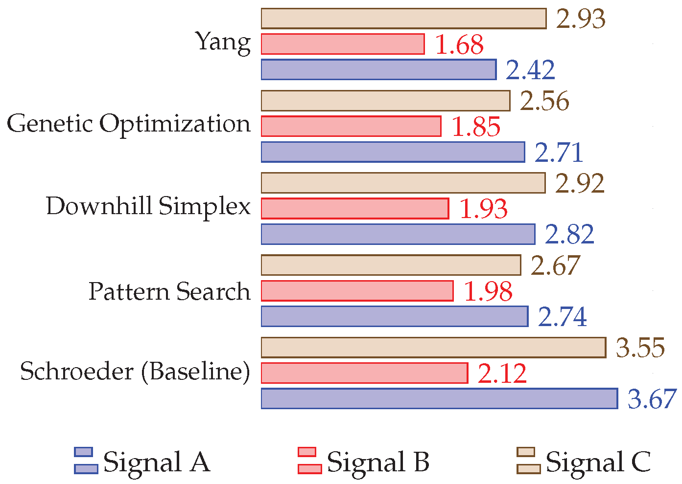
Figure 2.
Comparison of time domain behaviour of logarithmic and linear scaled multi-sine signals. CF values optimized according to Yang et al. [29].
Figure 2.
Comparison of time domain behaviour of logarithmic and linear scaled multi-sine signals. CF values optimized according to Yang et al. [29].

Figure 3.
Blockwise DFT with sliding Hann window.

Figure 4.
Standard deviation of 3600 consecutive impedance measurements, evaluated with different window length and types.
Figure 4.
Standard deviation of 3600 consecutive impedance measurements, evaluated with different window length and types.

Figure 5.
Measurement setup: Device under test, modified EISmeter and Host-PC.
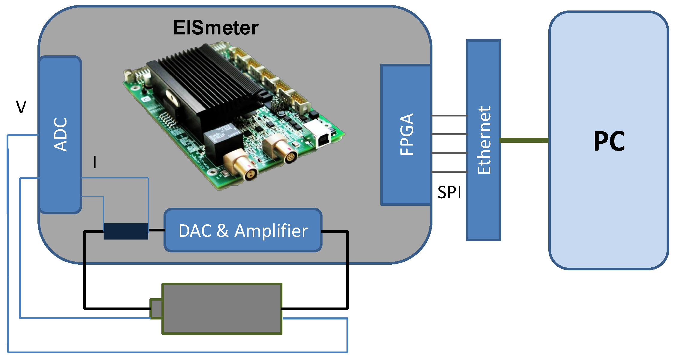
Figure 6.
Impedance measurement of 10 m reference shunt.From left to right: Comparison of mean values for multi- and stepped-sine, relative deviation for multi-sine, comparison of standard deviation. (Top row): Magnitude of Z (a–c). (Bottom row): Phase of Z (d–f).
Figure 6.
Impedance measurement of 10 m reference shunt.From left to right: Comparison of mean values for multi- and stepped-sine, relative deviation for multi-sine, comparison of standard deviation. (Top row): Magnitude of Z (a–c). (Bottom row): Phase of Z (d–f).

Figure 7.
(Left): Schematic of reference schematic circuit (reproduced from Nordmann et al. [34]). (Right): Nyquist plot of measurement results for multi-sine and stepped-sine measurement.
Figure 7.
(Left): Schematic of reference schematic circuit (reproduced from Nordmann et al. [34]). (Right): Nyquist plot of measurement results for multi-sine and stepped-sine measurement.

Figure 8.
(Left): Test setup with heating foil and temperature sensor on battery cell. (Right): Temperature behavior during C charge.
Figure 8.
(Left): Test setup with heating foil and temperature sensor on battery cell. (Right): Temperature behavior during C charge.

Figure 9.
(Top): Re(Z) (a) and Im(Z) (b) versus state of charge. Nyquist Plot of first and last spectrum (c). (Bottom): Calculated Kramers-Kronig residuals from Lin-KK tool [35] over frequency. (Left): Begin of Charge (d). (Right): End of Charge (e).
Figure 9.
(Top): Re(Z) (a) and Im(Z) (b) versus state of charge. Nyquist Plot of first and last spectrum (c). (Bottom): Calculated Kramers-Kronig residuals from Lin-KK tool [35] over frequency. (Left): Begin of Charge (d). (Right): End of Charge (e).

Figure 10.
(Top): Differential Change in Real Part of Impedance versus Charge. Frequency points and coloring: See legend of Figure 9a. (Bottom): Differential Voltage Analysis.
Figure 10.
(Top): Differential Change in Real Part of Impedance versus Charge. Frequency points and coloring: See legend of Figure 9a. (Bottom): Differential Voltage Analysis.

Table 1.
Multisine signals for crest factor (CF) optimization.
| Signal A | Signal B | Signal C | |
|---|---|---|---|
| 1 Hz | 1 Hz | 1 kHz | |
| 1 kHz | 1 kHz | 1 MHz | |
| Frequency distribution | quasi-logarithmic | linear | logarithmic |
| Number of frequency points | 21 | 21 | 21 |
| Number of samples | 96,000 | 96,000 | 96,000 |
| Length | 1 s | 1 s | 1 ms |
Table 2.
Properties of evaluated excitation signals for shunt measurement.
| Signal | Stepped-Sine | Multi-Sine |
|---|---|---|
| 1 Hz | 1 Hz | |
| 1 kHz | 1 kHz | |
| Frequency Distribution | quasi-logarithmic | |
| Frequency Points | 20 | 20 |
| Periods per Point | 10 | variable |
| RMS Current | mA | mA |
| Amplitude per Frequency Point | mA | mA |
| Peak Current Amplitude | mA | mA |
| Crest Factor | 1.41 | 2.528 |
| Signal Power | W | 561 W |
| Signal Length | s | 1 s |
| Signal Energy | mJ | mJ |
Pause intervals between frequency points excluded; Maximum of absolute value; At 10 mΩ pure-ohmic load.
© 2018 by the authors. Licensee MDPI, Basel, Switzerland. This article is an open access article distributed under the terms and conditions of the Creative Commons Attribution (CC BY) license (http://creativecommons.org/licenses/by/4.0/).
Share and Cite
MDPI and ACS Style
Zappen, H.; Ringbeck, F.; Sauer, D.U. Application of Time-Resolved Multi-Sine Impedance Spectroscopy for Lithium-Ion Battery Characterization. Batteries 2018, 4, 64. https://doi.org/10.3390/batteries4040064
AMA Style
Zappen H, Ringbeck F, Sauer DU. Application of Time-Resolved Multi-Sine Impedance Spectroscopy for Lithium-Ion Battery Characterization. Batteries. 2018; 4(4):64. https://doi.org/10.3390/batteries4040064
Chicago/Turabian StyleZappen, Hendrik, Florian Ringbeck, and Dirk Uwe Sauer. 2018. "Application of Time-Resolved Multi-Sine Impedance Spectroscopy for Lithium-Ion Battery Characterization" Batteries 4, no. 4: 64. https://doi.org/10.3390/batteries4040064
Note that from the first issue of 2016, this journal uses article numbers instead of page numbers. See further details here.