A Lithium-Ion Battery Capacity and RUL Prediction Fusion Method Based on Decomposition Strategy and GRU

Abstract

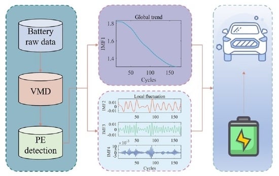
To safeguard the security and dependability of battery management systems (BMS), it is essential to provide reliable forecasts of battery capacity and remaining useful life (RUL). However, most of the current prediction methods use the measurement data directly to carry out prediction work, which ignores the objective measurement noise and capacity increase during the aging process of batteries. In this study, an integrated prediction method is introduced to highlight the prediction of lithium-ion battery capacity and RUL. This approach incorporates several techniques, including variational modal decomposition (VMD) with entropy detection, a double Gaussian model, and a gated recurrent unit neural network (GRU NN). Specifically, the PE−VMD algorithm is first utilized to perform a noise reduction process on the capacity data obtained from the measurements, and this results in a global degradation trend sequence and local fluctuation sequences. Afterward, the global degradation prediction model is established by employing the double Gaussian aging model proposed in this paper, and the local prediction models are built for each local fluctuation sequence by GRU NN. Lastly, the proposed hybrid prediction methodology is validated through battery capacity and RUL prediction studies on experimental data from three sources, and its accuracy is also compared with prediction algorithms from the recent related literature. Experimental results demonstrate that the proposed hybrid prediction method exhibits high precision in the predicting future capacity and RUL of lithium-ion batteries, along with strong robustness and predictive stability.

1. Introduction

Lithium-ion batteries are rechargeable batteries that use lithium ions as their primary component. They play an integral part in a variety of applications including electronic gadgets, electric vehicles (EVs), and renewable energy systems, owing to their remarkable characteristics such as fast charging, low maintenance, and environmental friendliness [1,2]. Despite also having a long lifespan, allowing them to be recharged and used multiple times before needing to be replaced, lithium-ion batteries can experience aging over time, which can lead to a decrease in their performance. Each charge and discharge cycle of a lithium-ion battery causes a small amount of wear and tear on the battery, and can cause permanent damage to its internal components, resulting in a decrease in capacity and lifespan. A lithium-ion battery is typically deemed to have reached its end of life (EOL) and needs to get recycled when its maximum discharge capacity has declined to 70% to 80% of its rated capacity. The battery cycles from the current to the EOL are defined as the remaining useful life (RUL). If the battery continues service after failure, it could even result in the risk of overheating and the potential for fire or explosion if not handled properly. Accurately predicting the capacity and RUL of lithium-ion batteries is indispensable in numerous applications and industries. It can supply the necessary upkeep and care to help mitigate potential risks and guarantee the secure and effective usage of lithium-ion batteries. As in the case of EVs, it is necessary to forecast the capacity and RUL of the battery for ensuring reliable and safe operation, as well as optimize charging and discharging strategies to extend the battery lifespan and improve performance. Therefore, developing reliable and precise methods to predict battery capacity and RUL is essential for the advancement and widespread adoption of technology.

Several scholars have focused on this significant issue that urgently needs to be addressed effectively, and many methods have been proposed. Model-based approaches [3,4,5,6,7,8,9], data-driven strategies [10,11,12,13,14,15,16,17,18,19,20,21], and hybrid prognostics [22,23,24,25,26,27,28] are the three main groups into which these methods may be categorized.

Model-based methods simplify the complex internal electrochemical reaction to reflect the operating characteristics of batteries. The electrochemical models (EM), equivalent circuit models (ECM), and empirical models are the three main model forecasting methods. For example, Xu et al. [3] developed a reduced pseudo-two-dimensional model with Pade approximation to identify the state of electrolyte decomposition in lithium-ion batteries. It could potentially improve the accuracy of battery capacity and RUL prediction. Sadabadi et al. [4] proposed an estimation algorithm of parameters based on an electrochemical model to design an RUL predictor. Their approach was to simulate the behavior of the batteries through an electrochemical model, and then propose a new metric to estimate the state of battery health. Although the EMs are capable of defining the battery’s degrading characteristics in terms of their internal mechanism and structure, they are typically developed for specific battery chemistries and designs, and their transferability to other battery systems can be limited. For the ECM, electrical components are used to simulate the internal chemical reaction of lithium-ion batteries to reflect the working properties of batteries. The estimation of parameters in the ECM is significantly aided by the Kalman filter (KF) and particle filter (PF). Duong et al. [5] discussed a heuristic Kalman filter, which integrated a PF with a KF for predicting the remaining useful life of lithium-ion batteries. Sun et al. [6] introduced a remaining charging electric quantity, and model parameters were identified online by a dual extended Kalman filter. While taking into account the aging inconsistency of lithium-ion battery packs, the proposed method improved the available capacity of the battery pack compared to conventional methods. Dong et al. [7] modeled the capacity decay of a battery as a Brownian motion process and took advantage of PF to estimate the drift parameter, which achieved a long-term RUL prognosis. Zhang et al. [8] were concerned with the particle impoverishment issue in unscented particle filter (UPF) to improve the forecast accuracy for batteries. However, the accuracy of the ECM is related to the number of electronic components and the accuracy of the identified parameters, making it difficult to develop an exact equivalent circuit model. The empirical model is formulated according to the concept of curve fitting, which posits that the capacity decay trajectory of batteries conforms to a certain mathematical function. Hong et al. [9] applied stochastic processes to RUL prediction, and a generalized Cauchy iterative model was proposed. This model incorporated the variability of the battery capacity degradation rate and the randomness of the RUL. Exponential models and polynomial models are also commonly used to fit the capacity decline trend of lithium-ion batteries. Nevertheless, deriving an accurate empirical model is a highly challenging task to track the battery capacity degradation trajectory, and the degradation patterns need to be uncovered from a large amount of a priori knowledge and experimental data.

Data-driven techniques involve the collection, preprocessing, and analysis of data to identify patterns and relationships between variables. They rely on historical data for prediction or decision making, without considering any prior knowledge or assumptions. Machine learning [10] and statistical methods are commonly used in data-driven technologies. Like the support vector machine (SVM) [11], multilayer perceptron (MLP) [12], and random vector functional link (RVFL) neural network [13], they play a significant role in various engineering applications. Data-driven techniques are also widely applied in the field of lithium-ion battery forecasting. For instance, Hu et al. [14] used a transformer neural network to build the forecasting model. Wu et al. [15] presented an improved random forest algorithm by particle swarm (PSO-RF) to obtain the optimal parametric solution. Zhang et al. [16] utilized a long short-term memory neural network (LSTM NN) to simulate capacity decay. A support vector regression (SVR) estimation framework was proposed by Wang et al. [17]. They introduced the quantum computing theory to the classical machine learning algorithms, and then applied it to extract aging characteristics from the charging curve. Li et al. [18] focused on extract the degradation features of the battery, and the Gaussian process regression (GPR) method was used to establish a mapping relationship between the extracted features and the RUL of the battery. Considering the impedance increase according to the degree of deterioration, Lee et al. [19] statistically analyzed the capacity decay data to find multiple decay features to train deep neural networks (DNN) to increase forecast precision. Ji et al. [20] combined the modified differential evolution algorithm (SADE) and the multiscale ensemble neural network (MESN), which predicts RUL from a monotonically decreasing capacity perspective, but ignores the possibility of sudden changes in capacity. Cadini et al. [21] suggested a multilayer perceptron (MLP) to construct measurement equations that could adaptively predict the EOL of batteries. These machine learning-based methods do not require a deep understanding of battery physics and chemistry principles, and they are simple to implement for predicting battery capacity and RUL. However, they sometimes could be restricted by the adequacy and accuracy of the available data, especially when the data contain noise, which is not representative of the actual operating conditions.

Prediction experiments with batteries have revealed that neither single model-based approaches nor data-driven techniques can completely overcome their shortcomings. As a result, hybrid forecasting methods have received increasing attention from researchers. Multiple data-driven integrated approaches and combined model and data-driven techniques, as well as combined multi-model approaches, are becoming mainstream in prognostics. For example, Zhao et al. [22] constructed a BLS–LSTM fusion forecasting network by creating enhancement nodes for the LSTM NN using the generalized learning system (BLS) algorithm. The BLS could generate feature nodes to enhance the mapping capabilities of the network. Chen et al. [23] chose to integrate BLS with a relevance vector machine (RVM), in which the BLS was used to preprocess the input data and reduce the dimensionality, while the RVM was used to establish the prediction model. Chen et al. [24] introduced the LSTM NN as a decay function of the Wiener process (WP), which could avoid the randomness of the WP degeneracy function. Zhang et al. [25] combined RVM with an improved aging model. The feature variables extracted by RVM were taken to build the aging prediction model. A logistic regression (LR) and PF were applied to a state-space model by Yu [26], which was based on a probabilistic indication. Yu [27] adopted a combination of multiscale logic regression (MLR) and GPR techniques, which captured the degradation behavior of the time-varying battery capacity. Considering the capacity regeneration point (CRP), Ma et al. [28] performed relevant tests before prediction. The predicted values of the autoregressive (AR) model were used as actual values and then were employed to update the double exponential model.

However, the drawback of the aforementioned methodologies is the almost direct use of recorded capacity data for study. The measured battery capacity data are usually contaminated by clutter and noise as a result of instrumentation errors and measurement interference factors. Directly predicting the battery’s future capacity and RUL employing measurement data with noise is tricky and unreliable. In addition, it is necessary to fully take into account the local capacity regeneration phenomenon generated during the charge–discharge cycles of the batteries, which will seriously affect the modeling of capacity deterioration and RUL forecasting. Therefore, the direct use of capacity time series with nonlinear and non-smooth characteristics for battery RUL prediction remains a large, challenging task. As a novel signal processing technique, variational modal decomposition (VMD) obtains baseband-smoothed intrinsic mode functions (IMFs) by pre-estimating the central pulsation frequency of each subseries. The decomposition process guarantees the independence of each mode and, therefore, offers powerful advantages for the decomposition of real signals. The entropy value of a signal determines its complexity and randomness. Thus, the VMD parameters can be updated according to this property of permutation entropy (PE).

Inspired by the aforementioned factors, this study proposes a new hybrid forecasting scheme that integrates model-driven and data-driven approaches to achieve precise estimations of both the capacity and RUL of lithium-ion batteries. The primary contributions might be emphasized as follows:

(1)

An innovative hybrid approach for capacity and RUL prediction is developed. The measured capacity data is decoupled by the VMD algorithm into a global degradation trend sequence and local fluctuation sequences, followed by a double Gaussian aging model to predict global degradation trends and a GRU NN to predict local changes. This hybrid method overcomes to some extent the effects of measurement noise and sudden changes in capacity.

(2)

The modal components are determined by PE detection and then adaptively categorized into different trend types, which safeguards the subsequent prediction and enhances the noise immunity of the forecasting system.

(3)

A novel double Gaussian model for battery capacity aging is proposed with excellent fitting properties, for which the Levenberg–Marquardt and PF (LM-PF) algorithm overcomes the parameter sensitivity problem. The learning rate of the GRU is optimized by the beetle antennae search (BAS) algorithm.

The remaining components of this paper are organized as follows: Section 2 focuses on clarifying the algorithm principles, including the optimized PE−VMD algorithm, improved double Gaussian model, and GRU NN; Section 3 describes the experimental procedure and steps, and introduces the experimental equipment and experimental data; the experimental results and discussions are shown in Section 4, which validates the predictive effectiveness of the proposed hybrid strategy; the pivotal conclusions are summarized in Section 5.

2. Methodology

2.1. Related Theory of VMD Algorithm

The VMD algorithm decomposes a signal into a finite number of modes, each of which represents a component of the signal with a specific frequency and amplitude. The main steps in the signal decomposition using VMD are as follows:

Step 1: The input signal $\mathrm{f}\left(\mathrm{t}\right)$ is decomposed into $\mathrm{K}$ eigenmode components ${\mathrm{u}}_{\mathrm{k}}(\mathrm{t})$ of different central frequencies and finite bandwidths by VMD, and ${\mathrm{u}}_{\mathrm{k}}(\mathrm{t})$ is defined as

$${\mathrm{u}}_{\mathrm{k}}\left(\mathrm{t}\right)={\mathrm{A}}_{\mathrm{k}}(\mathrm{t})\cos ({\mathsf{\varphi }}_{\mathrm{k}}(\mathrm{t})),$$

(1)

where ${\mathrm{A}}_{\mathrm{k}}(\mathrm{t})$ represents the instantaneous amplitude, ${\mathsf{\phi }}_{\mathrm{k}}(\mathrm{t})$ is the instantaneous phase, and $\mathrm{t}$ is the index of time.

Step 2: The one-sided spectrum is obtained by applying the Hilbert transform to ${\mathrm{u}}_{\mathrm{k}}(\mathrm{t})$.

$$(\mathsf{\delta }(\mathrm{t})+\frac{\mathrm{j}}{\mathsf{\pi }\mathrm{t}}){\mathrm{u}}_{\mathrm{k}}(\mathrm{t}),$$

(2)

where $\mathsf{\delta }(\mathrm{t})$ is the unit impulse, and $\mathrm{j}$ is an imaginary unit.

Step 3: The spectrums are modulated to the corresponding band range by

$$\left[\left(\mathsf{\delta }(\mathrm{t})+\frac{\mathrm{j}}{\mathsf{\pi }\mathrm{t}}\right){\mathrm{u}}_{\mathrm{k}}(\mathrm{t})\right]{\mathrm{e}}^{-\mathrm{j}{\mathsf{\omega }}_{\mathrm{k}}\mathrm{t}},$$

(3)

where ${\mathsf{\omega }}_{\mathrm{k}}$ is the center frequency.

Step 4: Calculating the ${\mathrm{L}}_2$ norm of the above signal, a constraint expression can be established as follows:

$$\begin{array}{l}\underset{\left\{{\mathrm{u}}_{\mathrm{k}}\right\} , \left\{{\mathsf{\omega }}_{\mathrm{k}}\right\}}{\min }\left\{{\displaystyle \sum _{\mathrm{k}}{‖{\partial }_{\mathrm{t}}\left[\left(\mathsf{\delta }(\mathrm{t})+\frac{\mathrm{j}}{\mathsf{\pi }\mathrm{t}}\right){\mathrm{u}}_{\mathrm{k}}(\mathrm{t})\right]{\mathrm{e}}^{-\mathrm{j}{\mathsf{\omega }}_{\mathrm{k}}\mathrm{t}}‖}_2^2}\right\}\\ \mathrm{s}.\mathrm{t}. {\displaystyle \sum _{\mathrm{k}}{\mathrm{u}}_{\mathrm{k}}=\mathrm{f}(\mathrm{t})}\end{array},$$

(4)

where $\left\{{\mathrm{u}}_{\mathrm{k}}\right\}=\left\{{\mathrm{u}}_1, \dots , {\mathrm{u}}_{\mathrm{K}}\right\}$ refers to the modal ensemble, $\left\{{\mathsf{\omega }}_{\mathrm{k}}\right\}=\left\{{\mathsf{\omega }}_1, \dots , {\mathsf{\omega }}_{\mathrm{K}}\right\}$ indicates central frequencies of the modes, ${\partial }_{\mathrm{t}}$ is the partial derivative for the variable $\mathrm{t}$, and $\mathrm{K}$ is the number of modals.

Step 5: Equation (4) is converted into an unconstrained problem using the penalty term $\mathsf{\alpha }$ and the Lagrange multiplier $\mathsf{\lambda }$, and the solution is as follows:

$$\begin{array}{l}\mathrm{L}\left(\left\{{\mathrm{u}}_{\mathrm{k}}\right\},\left\{{\mathsf{\omega }}_{\mathrm{k}}\right\},\mathsf{\lambda }\right)=\mathsf{\alpha }{{\displaystyle \sum _{\mathrm{k}}‖{\partial }_{\mathrm{t}}\left[\left(\mathsf{\delta }(\mathrm{t})+\frac{\mathrm{j}}{\mathsf{\pi }\mathrm{t}}\right){\mathrm{u}}_{\mathrm{k}}(\mathrm{t})\right]{\mathrm{e}}^{-\mathrm{j}{\mathsf{\omega }}_{\mathrm{k}}\mathrm{t}}‖}}_{2_{.}}^2\\ +{‖\mathrm{f}(\mathrm{t})-{\displaystyle \sum _{\mathrm{k}}{\mathrm{u}}_{\mathrm{k}}(\mathrm{t})}‖}_2^2+〈\mathsf{\lambda }(\mathrm{t}),\mathrm{f}(\mathrm{t})-{\displaystyle \sum _{\mathrm{k}}{\mathrm{u}}_{\mathrm{k}}(\mathrm{t})}〉\end{array}$$

(5)

Step 6: The optimal solution to Equation (5) is derived by employing the alternating direction multiplier method. To keep ${\mathrm{u}}_{\mathrm{k}}$ updated, the subproblem of the above equation is transformed into the problem of finding the minimal value of Equation (6).

$${\mathrm{u}}_{\mathrm{k}}{}^{\mathrm{n}+1}=\arg \min \left\{\mathsf{\alpha }{‖{\partial }_{\mathrm{t}}\left[\left(\mathsf{\delta }(\mathrm{t})+\frac{\mathrm{j}}{\mathsf{\pi }\mathrm{t}}\right){\mathrm{u}}_{\mathrm{k}}(\mathrm{t})\right]{\mathrm{e}}^{-\mathrm{j}{\mathsf{\omega }}_{\mathrm{k}}\mathrm{t}}‖}_2^2+{‖\mathrm{f}(\mathrm{t})-{\displaystyle \sum _{\mathrm{i}}{\mathrm{u}}_{\mathrm{i}}(\mathrm{t})+\frac{\mathsf{\lambda }(\mathrm{t})}{2}}‖}_2^2\right\}.$$

(6)

Step 7: The optimum solution for mode ${\mathrm{u}}_{\mathrm{k}}$ is formulated as follows:

$$\stackrel{}{{\stackrel{\wedge }{\mathrm{u}}}_{\mathrm{k}}^{\mathrm{n}+1}}(\mathsf{\omega })=\frac{\stackrel{}{\stackrel{}{\stackrel{\wedge }{\mathrm{f}}(\mathsf{\omega })}-{\displaystyle \sum _{\mathrm{i}\ne \mathrm{k}}\stackrel{}{{\stackrel{\wedge }{\mathrm{u}}}_{\mathrm{i}}\left(\mathsf{\omega }\right)+(\stackrel{\wedge }{\mathsf{\lambda }}(\mathsf{\omega })/2)}}}}{1+2\mathsf{\alpha }{(\mathsf{\omega }-{\mathsf{\omega }}_{\mathrm{k}})}^2},$$

(7)

where $\stackrel{\wedge }{\mathrm{f}}(\mathsf{\omega })$, $\stackrel{\wedge }{{\mathrm{u}}_{\mathrm{i}}}(\mathsf{\omega })$, $\stackrel{\wedge }{\mathsf{\lambda }}(\mathsf{\omega })$, and ${\stackrel{\wedge }{\mathrm{u}}}_{\mathrm{k}}^{\mathrm{n}+1}$ represent the Fourier transform of each variable.

2.2. PE Algorithm

The permutation entropy (PE) [29] is a powerful tool for analyzing data. It is mainly used to quantify the complexity and irregularity of time series data and is suitable for non-smooth signal analysis with good robustness. The PE algorithm works on the following principles:

(1)

A sequence of time series $\left\{\mathrm{X}\left(\mathrm{i}\right), \mathrm{i}=1, 2, \dots \mathrm{N}\right\}$ of length N is reconstructed in phase space and yields a matrix Y.

$$\mathrm{Y}=\left[\begin{array}{l}\mathrm{x}(1) \mathrm{x}(1+\mathrm{t}) \dots \mathrm{x}(1+(\mathrm{m}-1)\mathrm{t}\\ \mathrm{x}(2) \mathrm{x}(2+\mathrm{t}) \dots \mathrm{x}(2+(\mathrm{m}-1)\mathrm{t}\\ \mathrm{x}(\mathrm{j}) \mathrm{x}(\mathrm{j}+\mathrm{t}) \dots \mathrm{x}(\mathrm{j}+(\mathrm{m}-1)\mathrm{t}\\ ⋮\hspace{1em}\hspace{1em} ⋮ \hspace{1em}⋮ \hspace{1em}\hspace{1em}⋮\\ \mathrm{x}(\mathrm{k}) \mathrm{x}(\mathrm{k}+\mathrm{t}) \dots \mathrm{x}(\mathrm{k}+(\mathrm{m}-1)\mathrm{t}\end{array}\right],$$

(8)

where $\mathrm{m}$ is the embedding dimension, $\mathrm{t}$ is the delay time, and $\mathrm{k}=\mathrm{N}-(\mathrm{m}-1)$. Each row in the matrix $\mathrm{Y}$ is a reconstructed component, a total of $\mathrm{k}$.

(2)

Rearranging each reconstructed component in ascending order gives the column indices of the positions of the elements in the vector and forms a set of symbolic sequences.

$$\mathrm{S}(\mathrm{l})=\left\{{\mathrm{j}}_1,{\mathrm{j}}_2,\mathrm{\dots } {\mathrm{j}}_{\mathrm{m}}\right\},$$

(9)

where $\mathrm{l}=1, 2, \dots , \mathrm{k}$, $\mathrm{k}\le \mathrm{m}!$, and the total number of different symbol sequences is $\mathrm{m}!$.

(3)

Calculating the probability of each symbolic sequence, i.e., $\left\{{\mathrm{P}}_1, {\mathrm{P}}_2, \dots , {\mathrm{P}}_{\mathrm{k}}\right\}$, and the formula for calculating the permutation entropy of a time sequence X is

$${\mathrm{H}}_{\mathrm{p}\mathrm{e}}=-{\displaystyle \sum _{\mathrm{j}=1}^{\mathrm{k}}{\mathrm{P}}_{\mathrm{j}}\ln ({\mathrm{P}}_{\mathrm{j}})}.$$

(10)

(4)

When ${\mathrm{P}}_{\mathrm{j}}=1/\mathrm{m}!$, ${\mathrm{H}}_{\mathrm{p}\mathrm{e}}$ achieves a maximum value $\ln (\mathrm{m}!)$. Usually, ${\mathrm{H}}_{\mathrm{p}\mathrm{e}}$ can be normalized using $\ln (\mathrm{m}!)$:

$$0\le {\mathrm{H}}_{\mathrm{p}\mathrm{e}}=\frac{{\mathrm{H}}_{\mathrm{p}\mathrm{e}}}{\ln (\mathrm{m}!)}\le 1.$$

(11)

${\mathrm{H}}_{\mathrm{p}\mathrm{e}}$ is the final permutation entropy value, which takes values in the range [0, 1]. PE has found extensive applications in the fields of rotating machinery fault diagnosis [30] and cardiac monitoring [31]. The study by Rajabi et al. [32] demonstrated that a threshold of PE = 0.7 serves as a reasonable reference for fault detection. On the basis of this foundation, the threshold can be extended to the predictive research of lithium batteries and employed as a basis for distinguishing useful signals from noise.

2.3. Optimization of the VMD Algorithm with PE Detection

A higher entropy value means that the signal is more random. Conversely, the signal more regular and ordered. Therefore, the PE algorithm is applied for the detection of anomalous signals in this paper, which determines the number of modals of the VMD algorithm. The improved PF-VMD processes are displayed in Figure 1 and explained below.

(a)

The initial parameters are set for VMD and PE, where the initial number of decompositions $\mathrm{K}$ is set to 1.

(b)

VMD processing is performed on the input signal to generate IMFs, and the PE values of the resulting IMFs are calculated.

(c)

The presence of IMFs with PE values up to the threshold is verified.

(d)

If the conditions of the algorithm are met, the IMFs and the corresponding entropy values at that moment are output, and the VMD algorithm stops.

(e)

Otherwise, the modal component is updated and the number of decompositions $\mathrm{K}$ is increased by 1.

(f)

Steps (b) to (d) are repeated until the stopping condition is satisfied, and the algorithm stops.

2.4. LM-PF Algorithm for Optimising Double Gaussian Model

It is a well-known fact that the double exponential and polynomial models are commonly used as the battery capacity degradation pattern, which can be defined in Equations (12) and (13).

$$\stackrel{\wedge }{\mathrm{Q}}\left(\mathrm{k}\right)=\mathrm{a}\cdot \exp \left(\mathrm{b}\cdot \mathrm{k}\right)+\mathrm{c}\cdot \exp \left(\mathrm{d}\cdot \mathrm{k}\right),$$

(12)

$$\stackrel{\wedge }{\mathrm{Q}}\left(\mathrm{k}\right)={\mathrm{a}}_0+{\mathrm{a}}_1\cdot \mathrm{k}+{\mathrm{a}}_2\cdot {\mathrm{k}}^2+ \cdots +{\mathrm{a}}_{\mathrm{n}}\cdot {\mathrm{k}}^{\mathrm{n}-1},$$

(13)

where $\left(\mathrm{a}, \mathrm{b}, \mathrm{c}, \mathrm{d}\right)$ and $\left({\mathrm{a}}_0, {\mathrm{a}}_1, \cdots , {\mathrm{a}}_{\mathrm{n}}\right)$ are the parameters of these two models; $\stackrel{\wedge }{\mathrm{Q}}\left(\mathrm{k}\right)$ represents the capacity at the k-th cycle. From the mathematical analysis, we can find that the double exponential model applies provided that the trend of the fitted object approximates the exponential distribution. The trend of this model is strongly influenced by the attenuation parameters $\mathrm{b}$ and $\mathrm{d}$. When the absolute values of these two parameters are small, the trend of the double exponential model is close to a linear variation, resulting in a large fitting error. The accuracy of a polynomial model is related to its order, and it is often quite tricky to choose the best a priori order. When the order chosen is high, over-fitting problems are prone to occur.

In view of the above, this paper proposes an innovative double Gaussian model to describe the battery capacity decay process, defined as follows:

$$\stackrel{\wedge }{\mathrm{Q}}\left(\mathrm{k}\right)={\mathsf{\alpha }}_1\cdot \exp \left(-\frac{\mathrm{k}-{\mathsf{\beta }}_1}{{\mathsf{\lambda }}_1}\right)+{\mathsf{\alpha }}_2\cdot \exp \left(-\frac{\mathrm{k}-{\mathsf{\beta }}_2}{{\mathsf{\lambda }}_2}\right),$$

(14)

where $\mathrm{k}$ is the cycle of charge–discharge, $\stackrel{\wedge }{\mathrm{Q}}\left(\mathrm{k}\right)$ denotes battery capacity, and ${\mathsf{\alpha }}_1, {\mathsf{\beta }}_1, {\mathsf{\lambda }}_1, {\mathsf{\alpha }}_2, {\mathsf{\beta }}_2, {\mathsf{\lambda }}_2$ are the initial parameters of the double Gaussian model. Since the battery capacity decrease can be approximated as a Gaussian distribution concerning the number of cycles, this characterized capacity decay adopting a weighted sum of two Gaussian models is accurate and feasible. Yet, the increase in attenuation parameters also causes an element of complexity in identification. The Levenberg–Marquardt (LM) algorithm is popularly deployed for solving unconstrained nonlinear least squares problems. It is insensitive to overparameterization problems and can effectively handle redundant parameter problems. The particle filter (PF) is a probability statistics algorithm that calculates the sample mean of a set of particles to estimate the parameter being identified.

Therefore, in this work, a double Gaussian capacity fading model is constructed on the basis of the global decay sequence using the LM-PF algorithm to predict the global deterioration trend. The algorithm has the following steps:

Step 1:

The LM algorithm is applied to obtain the initial ${\mathrm{X}}_0=\left[{\mathsf{\alpha }}_1, {\mathsf{\beta }}_1, {\mathsf{\lambda }}_1, {\mathsf{\alpha }}_2, {\mathsf{\beta }}_2, {\mathsf{\lambda }}_2\right]$ for PF.

Step 2:

The set of particles ${\left\{{\mathrm{X}}_0^{\mathrm{i}}\right\}}_{\mathrm{i}=0}^{\mathrm{N}}, \mathrm{i}=\left(1,\cdots ,\mathrm{N}\right)$ is generated from the prior distribution $\mathrm{P}\left({\mathrm{X}}_0\right)$, where $\mathrm{N}$ denotes the whole amount of particles, and all particles are initialized with a weight of $W_0^{\mathrm{i}}=\frac{1}{\mathrm{N}}$.

Step 3:

${\mathrm{X}}_{\mathrm{k}}^{\mathrm{i}}\sim \mathrm{q}\left({\mathrm{X}}_{\mathrm{k}}^{\mathrm{i}}|{\mathrm{X}}_{0:\mathrm{k}-1}^{\mathrm{i}},Z_{\mathrm{k}}\right)$ is updated to get a new set of particles ${\mathrm{X}}_{\mathrm{k}}^{\mathrm{i}}$, where $\mathrm{k}=\left(1,\cdots ,\mathrm{K}\right)$ is the operating cycle, and $\mathrm{K}$ is the complete amount of aging cycle; $\mathrm{q}\left({\mathrm{X}}_{\mathrm{k}}^{\mathrm{i}}|{\mathrm{X}}_{0:\mathrm{k}-1}^{\mathrm{i}},Z_{\mathrm{k}}\right)$ represents the importance density function.

Step 4:

The important weight is calculated by Equation (15) for each particle in the particle set, and the weights are normalized according to Equation (16).

$$W_{\mathrm{k}}^{\mathrm{i}}=W_{\mathrm{k}-1}^{\mathrm{i}}\frac{\mathrm{P}\left(Z_{\mathrm{k}}|{\mathrm{X}}_{\mathrm{k}}^{\mathrm{i}}\right)\mathrm{P}\left({\mathrm{X}}_{\mathrm{k}}|{\mathrm{X}}_{\mathrm{k}-1}^{\mathrm{i}}\right)}{\mathrm{q}\left({\mathrm{X}}_{\mathrm{k}}^{\mathrm{i}}|{\mathrm{X}}_{\mathrm{k}-1}^{\mathrm{i}},Z_{1:\mathrm{k}}\right)}.$$

(15)

$$W_{\mathrm{k}}^{\prime }\left({\mathrm{X}}_{0:\mathrm{k}}^{\mathrm{i}}\right)=\frac{W_{\mathrm{k}}\left({\mathrm{X}}_{0:\mathrm{k}}^{\mathrm{i}}\right)}{{\displaystyle \sum _{\mathrm{i}=1}^{\mathrm{N}}{W}_{\mathrm{k}}\left({\mathrm{X}}_{0:\mathrm{k}}^{\mathrm{i}}\right)}}.$$

(16)

Step 5:

A fresh batch of particles $\left\{{\stackrel{\wedge }{\mathrm{X}}}_{1:\mathrm{K}}^{\mathrm{i}}\right\}, \mathrm{i}=\left(1,\cdots ,\mathrm{N}\right)$ is created by resampling, where ${\stackrel{\wedge }{\mathrm{X}}}_{\mathrm{k}}^{\mathrm{i}}$ is constructed from an estimate of the model parameters for particle $\mathrm{i}$ at cycle number $\mathrm{k}$.

Step 6:

An estimate of the capacity is obtained.

$${\stackrel{\wedge }{\mathrm{Q}}}_{\mathrm{k}}^{\mathrm{i}}=\mathrm{h}\left({\stackrel{\wedge }{\mathrm{X}}}_{\mathrm{k}}^{\mathrm{i}}\right),$$

(17)

where ${\stackrel{\wedge }{\mathrm{Q}}}_{\mathrm{k}}^{\mathrm{i}}$ refers the estimated battery capacity of particle $\mathrm{i}$, and $\mathrm{h}\left(\cdot \right)$ is the double Gaussian observation equation.

2.5. GRU NN and BAS Algorithm

The gated recurrent unit neural network (GRU NN) [33] is an enhanced form of the recurrent neural network (RNN) that exhibits superior long-term sequence memorization capabilities compared to the standard RNN. It is as effective as LSTM NN in solving the gradient explosion or disappearance problem of simple RNNs. Unlike the LSTM NN, the forget and input gates are synthesized into one update gate in GRU NN, and only one hidden state is given to pass information. Because GRU NN features an easier design, less variables, and higher convergence, it may be considered an excellent variation of LSTM NN. The basic structure of the GRU NN is shown in Figure 2.

The GRU NN’s fundamental unit is formed by the update gate and the reset gate. How much of the new candidate state should be joined to the existing hidden state is decided by the update gate. The calculated update gate value obtained is large, i.e., that the output of the previously hidden layer has a great impact on the current hidden layer. The reset gate is intended to govern how much of the previously hidden state should be forgotten, with a smaller value indicating that more information is being ignored, thus reducing the reliance on past information. For a GRU cell, the formulae for calculating the gating mechanisms and state processes are described below.

The input to the GRU NN is formed by the input ${\mathrm{x}}_{\mathrm{t}}$ at time $\mathrm{t}$ and the previous hidden state ${\mathrm{h}}_{\mathrm{t}-1}$. The hidden layer state contains information about the previous node.

The gating states of the reset and update gates are acquired by Equations (18) and (19), respectively.

$${\mathrm{r}}_{\mathrm{t}}=\mathsf{\sigma }({\mathrm{x}}_{\mathrm{t}}{\mathsf{\omega }}_{\mathrm{x}\mathrm{r}}+{\mathrm{h}}_{\mathrm{t}-1}{\mathsf{\omega }}_{\mathrm{h}\mathrm{r}}+{\mathrm{b}}_{\mathrm{r}}).$$

(18)

$${\mathrm{z}}_{\mathrm{t}}=\mathsf{\sigma }({\mathrm{x}}_{\mathrm{t}}{\mathsf{\omega }}_{\mathrm{x}\mathrm{z}}+{\mathrm{h}}_{\mathrm{t}-1}{\mathsf{\omega }}_{\mathrm{h}\mathrm{z}}+{\mathrm{b}}_{\mathrm{z}}).$$

(19)

The candidate hidden layer states are derived from the following equation:

$${\tilde{\mathrm{h}}}_{\mathrm{t}}=\tanh ({\mathrm{x}}_{\mathrm{t}}{\mathsf{\omega }}_{\mathrm{h}\mathrm{x}}+{\mathrm{r}}_{\mathrm{t}}{\mathrm{h}}_{\mathrm{t}-1}{\mathsf{\omega }}_{\mathrm{h}\mathrm{h}}+{\mathrm{b}}_{\mathrm{h}}).$$

(20)

when ${\mathrm{r}}_{\mathrm{t}}$ converges to 0, GRU NN discards the ${\mathrm{h}}_{\mathrm{t}-1}$ at moment $\mathrm{t}-1$, leaving the current input information; when ${\mathrm{r}}_{\mathrm{t}}$ converges to 1, the hidden layer information is retained.

The output ${\mathrm{y}}_{\mathrm{t}}$ of the hidden layer node is computed at moment $\mathrm{t}$, and the current hidden state ${\mathrm{h}}_{\mathrm{t}}$ is passed to the next node.

$${\mathrm{h}}_{\mathrm{t}}=(1-{\mathrm{z}}_{\mathrm{t}}){\mathrm{h}}_{\mathrm{t}-1}+{\mathrm{z}}_{\mathrm{t}}{\tilde{\mathrm{h}}}_{\mathrm{t}},$$

(21)

$${\mathrm{y}}_{\mathrm{t}}=\mathsf{\sigma }({\mathsf{\omega }}_{\mathrm{o}}{\mathrm{h}}_{\mathrm{t}}),$$

(22)

where $\mathsf{\omega }$ represents the weighting factor, $\mathrm{b}$ refers to bias, $\mathsf{\sigma }$ is the sigmoid function, and $\tanh \left(\mathrm{x}\right)$ is the hyperbolic tangent function; they are used to implement gate control functionality.

$$\mathsf{\sigma }(\mathrm{x})=\frac{1}{1+\exp (-\mathrm{x})}.$$

(23)

$$\tanh (\mathrm{x})=\frac{\exp (\mathrm{x})-\exp (-\mathrm{x})}{\exp (\mathrm{x})+\exp (-\mathrm{x})}.$$

(24)

In addition, the complex and diverse sequences of local fluctuations require the GRU model to make matching learning rate corrections. In this section, the beetle antennae search (BAS) algorithm is implemented to optimize the learning rate of the GRU NN. The BAS algorithm is inspired by the search behavior of beetles that move around in the search space. The main core process consists of two aspects. The beetle position is initialized according to Equation (25).

$$\left\{\begin{array}{l}\mathrm{i}=\mathrm{r}\mathrm{a}\mathrm{n}\mathrm{d}\mathrm{s}\left(\mathrm{n},1\right); \mathrm{i}=\mathrm{i}/\mathrm{n}\mathrm{o}\mathrm{r}\mathrm{m}\left(\mathrm{i}\right) \\ {\mathrm{X}}_{\mathrm{L}}=\mathrm{X}+\mathrm{D}\ast \left(\mathrm{i}/2\right); {\mathrm{X}}_{\mathrm{R}}=\mathrm{X}-\mathrm{D}\ast \left(\mathrm{i}/2\right)\end{array}\right.,$$

(25)

where $\mathrm{i}$ is a random vector generated in $\mathrm{n}$ dimensional space, $\mathrm{r}\mathrm{a}\mathrm{n}\mathrm{d}\mathrm{s}\left(\right)$ denotes the random function, and $\mathrm{n}\mathrm{o}\mathrm{r}\mathrm{m}\left(\right)$ refers to the normalization function. ${\mathrm{X}}_{\mathrm{L}}$ is the left coordinate, and ${\mathrm{X}}_{\mathrm{R}}$ is the right coordinate; $\mathrm{X}$ is the coordinate of the center of mass, and $\mathrm{D}$ is the distance between the left and right coordinates.

The fitness value is calculated using Equation (26), and the best position is updated accordingly.

$$\left\{\begin{array}{l}{\mathrm{f}}_{\mathrm{L}}=\mathrm{f}\left({\mathrm{X}}_{\mathrm{L}}\right); {\mathrm{f}}_{\mathrm{R}}=\mathrm{f}\left({\mathrm{X}}_{\mathrm{R}}\right)\\ \mathrm{X}=\mathrm{X}-\mathrm{s}\ast \mathrm{i}\ast \mathrm{s}\mathrm{i}\mathrm{g}\mathrm{n}\left({\mathrm{f}}_{\mathrm{L}}-{\mathrm{f}}_{\mathrm{R}}\right)\end{array}\right.,$$

(26)

where ${\mathrm{f}}_{\mathrm{L}}$ and ${\mathrm{f}}_{\mathrm{R}}$ are the function values corresponding to the left and right coordinates, respectively. $\mathrm{f}\left(\right)$ is the objective function, $\mathrm{s}$ represents the step size, and $\mathrm{s}\mathrm{i}\mathrm{g}\mathrm{n}\left(\right)$ is the sign function. After optimization of the learning rate, the GRU NN can track the fluctuating changes of sequences remarkably effectively.

3. Experimental Setup

In this study, the suggested hybrid prediction method is validated on the battery data gathered from NASA, the University of Maryland, and a custom experimental platform. Experimental data were measured by the high-performance battery test platform, hereafter referred to as S5. The NASA Ames Research Center provides a dataset [34] generated through accelerated life experiments. The capacity data of battery 5 and battery 6, which have been publicly released, were selected as the research object of this study. Data from the last battery, CX2-37 [35], were obtained from CALCE at the University of Maryland in an aging experiment. In addition, the EOL threshold was standardized uniformly at 70% of the rated capacity. The experimental data were equally divided, with the training and test sets being split for training the prediction model and validating the performance.

3.1. Laboratory Apparatus and Experiment Data

Our group has developed a comprehensive battery test system in the laboratory of AQNU University, comprising an upper computer, battery cell testing equipment, and a thermostat. The upper computer is used for recording and saving battery experimental data, and the battery cell testing equipment can perform tests in various working conditions due to its high responsiveness, high accuracy, and high efficiency. The experimental apparatus is shown in Figure 3.

Four differentiated battery cell data were employed to demonstrate the robustness and efficacy of the method proposed in this work. The aging data of battery S5 differed from that of NASA batteries and CALCE battery data, and there were several main reasons for this difference:

(1)

The 18650 cylindrical batteries include batteries S5, 5, and 6, while CX2-37 is a rectangular battery. The anode and cathode of battery S5 consist of graphite and LiFePO₄, while batteries 5 and 6 have a graphite anode and an LNCA cathode material. In contrast, CX2-37 utilizes LiCoO₂ as the cathode material. Moreover, the battery S5 is rated at 2.4 Ah; thus, the EOL criterion is designed as 1.68 Ah. Batteries 5 and 6 have a rated capacity of 2 Ah, with a 1.4 Ah EOL criterion. The rated capacity of CX2-37 is only 1.35 Ah, with its EOL threshold considered to be 0.945 Ah.

(2)

The aging test of battery S5 was tested at a 25 °C constant temperature; the datasets for batteries 5 and 6 were collected at a 24 °C constant temperature, while that of CX2-37 was tested at room temperature.

(3)

A constant current of 1.2 A was applied to charge the battery S5 up to 4.2 V, and then the voltage was kept constant at 4.2 V until the current decreased to 48 mA. The discharge process involved applying a 2.4 A constant current, and the voltage was discharged to 3.2 V. NASA batteries 5 and 6 were charged at a 1.5 A constant current; their voltage rose to 4.2 V, and then the voltage was maintained constant at 4.2 V until the current fell to 20 mA. The discharge procedure comprised the provision of a 2 A constant current and lowering the voltage to 2.7 V and 2.5 V, respectively. CX2-37 was charged at a constant current rate of 0.5 C to 4.2 V, and then the voltage was maintained until the current dropped to 0.05 A. It was discharged at a constant current rate of 1 C until the voltage fell to 2.7 V.

Figure 4 depicts the capacity data for battery S5, batteries 5 and 6, and CX2-37. As can be observed, the laboratory test results and the NASA aging datasets show that the capacity degraded with the increasing number of charge and discharge cycles up to the failure threshold. Furthermore, the capacity decay trajectory occasionally showed random irregular jumps due to numerous disturbances in the measurement process and unavoidable local capacity increases. However, as the entire aging test of the S5 was carried out in a thermostat, the decay trend was more stable.

3.2. Experimental Procedures

To assess the performance of the suggested hybrid prediction algorithm, predictive experiments were designed. The experiments in this paper consisted of two parts: battery future capacity prediction and remaining life prediction. The exact steps of the experiment are shown in Figure 5 and described below.

Step 1:

On the basis of the experimental data, the decomposition number and IMFs for capacity data were obtained by the improved PE−VMD algorithm.

Step 2:

The derived IMFs were adaptively divided into global degradation trend sequence and local fluctuation sequences according to their PE values.

Step 3:

Both the global degenerate trend sequence and the local fluctuation sequences were equally divided into the corresponding training and testing sets.

Step 4:

A double Gaussian capacity fading model was constructed to predict the global deterioration trend on the basis of the training set of the global degradation trend sequence adopting the LM-PF algorithm.

Step 5:

The training set of local fluctuation sequences was utilized, and the GRU local prediction model was trained to capture the local variations in capacity. The BAS algorithm was responsible for optimizing the learning rate of the GRU model.

Step 6:

The test set data were input, and the future global trend and future local fluctuation data were predicted by the double Gaussian capacity degradation model and GRU local prediction model, respectively.

Step 7:

The final capacity prediction result was generated by adding the predicted future local fluctuation data to the future global trend data.

Step 8:

The RUL was calculated from the EOL values.

3.3. Evaluation Criteria

To evaluate the precision of the suggested approach, the mean absolute percentage error (MAPE) [16], root-mean-square error (RMSE) [22], and Pearson correlation analysis method [22] were selected as evaluation metrics. Furthermore, the absolute error (AE) [23] was also used in the RUL prediction results for assessment. These metrics are presented as follows:

$$\mathrm{M}\mathrm{A}\mathrm{P}\mathrm{E}=\frac{1}{\mathrm{n}-\mathrm{k}}{\displaystyle \sum _{\mathrm{i}=\mathrm{k}}^{\mathrm{n}}\left|\frac{\widehat{{\mathrm{Q}}_{\mathrm{i}}}-{\mathrm{Q}}_{\mathrm{i}}}{{\mathrm{Q}}_{\mathrm{i}}}\right|}\times 100\%,$$

(27)

$$\mathrm{R}\mathrm{M}\mathrm{S}\mathrm{E}=\sqrt{\frac{1}{\mathrm{n}-\mathrm{k}}{\displaystyle \sum _{\mathrm{i}=\mathrm{k}}^{\mathrm{n}}{\left(\widehat{{\mathrm{Q}}_{\mathrm{i}}}-{\mathrm{Q}}_{\mathrm{i}}\right)}^2}},$$

(28)

$${\mathrm{R}}^2=1-\frac{{\displaystyle {\sum }_{\mathrm{i}=\mathrm{k}}^{\mathrm{n}}{\left({\mathrm{Q}}_{\mathrm{i}}-\widehat{\mathrm{I}\mathrm{M}{\mathrm{F}}_{\mathrm{i}}}\right)}^2}}{{\displaystyle {\sum }_{\mathrm{i}=\mathrm{k}}^{\mathrm{n}}{\left({\mathrm{Q}}_{\mathrm{i}}-\overline{\mathrm{I}\mathrm{M}{\mathrm{F}}_{\mathrm{i}}}\right)}^2}},$$

(29)

$$\mathrm{A}\mathrm{E}=\left|\mathrm{R}\mathrm{U}{\mathrm{L}}_{\mathrm{t}\mathrm{r}\mathrm{u}\mathrm{e}}-\mathrm{R}\mathrm{U}{\mathrm{L}}_{\mathrm{p}\mathrm{r}\mathrm{e}\mathrm{d}\mathrm{i}\mathrm{c}\mathrm{t}\mathrm{e}\mathrm{d}}\right|,$$

(30)

where ${\mathrm{Q}}_{\mathrm{i}}$ is the real capacity, and $\widehat{{\mathrm{Q}}_{\mathrm{i}}}$ is the predicted capacity. The number of cycles is $\mathrm{i}$; $\mathrm{n}$ denotes all prediction cycles, and $\mathrm{k}$ represents the starting point of the forecast. $\mathrm{R}\mathrm{U}{\mathrm{L}}_{\mathrm{t}\mathrm{r}\mathrm{u}\mathrm{e}}$ is the actual RUL, and $\mathrm{R}\mathrm{U}{\mathrm{L}}_{\mathrm{p}\mathrm{r}\mathrm{e}\mathrm{d}\mathrm{i}\mathrm{c}\mathrm{t}\mathrm{e}\mathrm{d}}$ indicates the predicted RUL. Generally speaking, a lower value of MAPE/RMSE/AE denotes better performance of the algorithm. ${\mathrm{R}}^2$ represents the correlation coefficient between ${\mathrm{Q}}_{\mathrm{i}}$ and IMFs. It was adopted to gauge the degree of correlation between the IMFs and capacity. The experiments were carried out using MATLAB 2020b.

4. Experimental Verification and Analysis

4.1. Battery Capacity Decomposition Based on PE−VMD

This section uses PE−VMD to decompose the raw capacity data for battery S5, batteries 5 and 6, and CX2-37. The decomposition process of these three types of batteries is recorded in

Table 1. Decomposition process of four types of batteries regarding the PE method.

(a) Battery S5
IMFs	IMF1		IMF2		IMF3		IMF4
K	Hpe	R2	Hpe	R2	Hpe	R2	Hpe	R2
K = 1	0.1575	0.9995
K = 2	0.1445	0.9802	0.2995	0.7015
K = 3	0.1373	0.9801	0.3022	0.7021	0.6042	0.0129
K = 4	0.0412	0.9799	0.2719	0.7121	0.3622	0.0625	0.7102	0.0122
(b) Battery 5
IMFs	IMF1		IMF2		IMF3		IMF4
K	Hpe	R2	Hpe	R2	Hpe	R2	Hpe	R2
K = 1	0.0832	0.9982
K = 2	0.0885	0.9981	0.6475	0.0642
K = 3	0.0542	0.9977	0.4435	0.1163	0.6485	0.0517
K = 4	0.0542	0.9977	0.4409	0.1156	0.6386	0.0514	0.7519	0.0312
(c) Battery 6
IMFs	IMF1		IMF2		IMF3
K	Hpe	R2	Hpe	R2	Hpe	R2
K = 1	0.1027	0.9963
K = 2	0.0832	0.9961	0.6359	0.0792
K = 3	0.0387	0.9955	0.4841	0.1179	0.7651	0.0518
(d) Battery CX2-37
IMFs	IMF1		IMF2		IMF3		IMF4
K	Hpe	R2	Hpe	R2	Hpe	R2	Hpe	R2
K = 1	0.3944	0.9994
K = 2	0.2920	0.9985	0.5623	0.0726
K = 3	0.1533	0.9984	0.4554	0.0740	0.6097	0.0285
K = 4	0.0771	0.9981	0.3956	0.0793	0.5845	0.0366	0.8078	0.0265

. Evaluation indicators include ${\mathrm{H}}_{\mathrm{p}\mathrm{e}}$ and ${\mathrm{R}}^2$, where ${\mathrm{H}}_{\mathrm{p}\mathrm{e}}$ refers to the entropy value of the IMFs, and ${\mathrm{R}}^2$ indicates the level of correlation of IMFs with original capacity. When ${\mathrm{H}}_{\mathrm{p}\mathrm{e}}$ of the IMFs reaches the threshold, it indicates that the input signal was sufficiently decomposed, and the VMD algorithm was stopped. Figure 6 presents the outcomes of the decomposition for the four typical batteries.

The decomposition process is shown in Table 1. PE−VMD performed a four-layer decomposition on battery S5, battery 5, and CX2-37, while battery 6 reached the ${\mathrm{H}}_{\mathrm{p}\mathrm{e}}$ threshold at the third layer of decomposition before stopping. IMF1 had the smallest ${\mathrm{H}}_{\mathrm{p}\mathrm{e}}$ value, whereas the ${\mathrm{R}}^2$ value was the largest and close to 1. This suggests that IMF1 was smoother and highly positively correlated with the original capacity. As the value of K increased, ${\mathrm{H}}_{\mathrm{p}\mathrm{e}}$ of the recently acquired IMF components gradually increased approaching the ${\mathrm{H}}_{\mathrm{p}\mathrm{e}}$ threshold, and their ${\mathrm{R}}^2$ tended to 0.

Figure 6 displays the results of the decomposition of battery S5, batteries 5 and 6, and CX2-37 by the PE−VMD algorithm. It can be obviously observed that the low-frequency component IMF1 exhibited a favorable monotonic decline, effectively preserving the trend of global degradation of the original capacity. Therefore, IMF1 was taken as the global trend degradation sequence. The remaining high-frequency components presented random oscillations, and these modal components represented local capacity regeneration with measurement error disturbances, which in turn made up the local fluctuation sequences. The decomposition results were consistent with the decomposition process in Table 1.

4.2. Capacity Prediction

In this study, the first 50% of the battery lifecycle was used as training data to construct a hybrid predictive model, while the remaining portion served as the test data. The global degradation sequence derived from the double Gaussian capacity degradation model prediction and the local fluctuation sequences predicted by GRU were integrated to form the predicted future capacity. The prognosis results of capacity are depicted in Figure 7, and

Table 2. Statistical errors of the prediction results.

Battery	RMSE	MAPE (%)
Battery S5	0.0103	0.4288
Battery B5	0.0083	0.4555
Battery B6	0.0142	0.6446
Battery CX2-37	0.0053	0.4289

reports the forecast errors for the four batteries.

The prediction results for battery S5, batteries 5 and 6, and battery CX2-37 clearly demonstrate that the suggested method allowed for precision forecasting of capacity. What is remarkable is that the proposed approach also appropriately captured the respective capacity jumping points. The impact of prognostic errors due to localized capacity increases was reduced.

This conclusion is strengthened by the statistical errors in Table 2. The $\mathrm{R}\mathrm{M}\mathrm{S}\mathrm{E}$ and $\mathrm{M}\mathrm{A}\mathrm{P}\mathrm{E}$ were below 0.02 and 1%, respectively, in the four case studies, which is an extremely small deviation, indicating that the predicted capacity values exhibited a high degree of similarity to the actual capacity values. It is also worth noting that, compared to batteries 5 and 6, battery CX2-37 offered a greater prediction accuracy employing the suggested method. This is because the aging data for battery CX2-37 were relatively smooth and stable, while the aging data for batteries 5 and 6 fluctuated dramatically.

To further investigate the validity of the proposed methodology, a new comparative experiment was considered on the basis of the existing battery data. Specifically, the performance of the suggested approach was separately compared with the PF technique and the GRU NN. In particular, the PF technique needed to be combined with a double Gaussian model. PF and individual GRU NN provided predictions on the raw measurement data, respectively, which were not processed by VMD. The comparison prediction results are displayed in Figure 8, and

Table 3. Prediction errors in the comparative experiment.

Battery	Algorithm	RMSE	MAPE (%)
Battery S5	PF	0.0173	0.7342
	GRU	0.0435	1.8197
Battery 5	PF	0.0172	0.8059
	GRU	0.0149	0.8081
Battery 6	PF	0.0243	1.0916
	GRU	0.0243	1.2754
Battery CX2-37	PF	0.0109	0.8720
	GRU	0.0101	0.8022

summarizes the prediction outcomes of the comparison method for all batteries.

The comparison results reveal that the capacity estimated by the suggested hybrid approach was closer to the actual capacity than the other two comparison methods, PF and GRU NN, across the four battery case studies. The predictions of the PF technique can roughly matched the battery capacity decay curve, thanks to the good fitting properties of the double Gaussian model. However, it was not possible to track capacity mutation points. Compared to PF technology, GRU NN captured changes in capacity degradation dynamics with its superior time sequence processing capabilities. Nevertheless, there was a gradual deviation from the true declining trend in capacity in the later stages of the prognosis.

The statistical errors reported in Table 3 illustrate a further problem. PF ignored the prediction of capacity increase points, while GRU NN ignored the distortion in late capacity forecasts. Although the prediction errors for both were small values, there was no significant difference between their prediction errors. Overall, the proposed method produced the smallest $\mathrm{R}\mathrm{M}\mathrm{S}\mathrm{E}$ and $\mathrm{M}\mathrm{A}\mathrm{P}\mathrm{E}$ in all four cases, which reflects a considerable improvement in the forecast errors by the proposed method.

4.3. RUL Prediction

Accurate RUL prediction is another critical issue to be overcome in prognostics and health management (PHM) for lithium-ion batteries. On the basis of the existing work, the RUL prediction effectiveness of the suggested hybrid model was researched with the four batteries mentioned above. The EOL cycles for battery S5, batteries 5 and 6, and CX2-37 were 137, 54, 43, and 1021, respectively. The capacity data used for RUL prediction should exceed 70% of the rated capacity, and the predictive results of all cases are shown in Figure 9.

It can be seen that, in this case, the dynamic changes in the capacity of the four batteries could still be captured in perfect time by the proposed method. The deterioration patterns of the expected capacity and the real capacity were roughly the same. This conclusion is verified by the prediction errors in

Table 4. Prediction errors of the RUL for the four batteries.

Battery	EOL Cycle	Actual RUL	Predicted RUL	AE
Battery S5	292	137	138	1
Battery 5	124	54	54	0
Battery 6	108	43	42	1
Battery CX2-37	1021	436	434	2

. The predicted RUL for batteries S5 and 6 was one cycle later and one cycle ahead of the true RUL, respectively. The RUL prediction error for battery CX2-37 was two cycles, whereas the predicted RUL for battery 5 was consistent with the actual RUL. It may, therefore, be concluded that the needs of battery RUL prediction can be met by the proposed method.

To further illustrate the superiority of the proposed method in battery RUL prediction, a comparative test with algorithms proposed in the recent related literature was performed. In order not to lose generality, the dataset of batteries 5 and 6 from the NASA database were selected for comparison with the recent related methods. All considered comparison methods unfolded RUL predictions at different stages.

Table 5. Comparison results of the proposed method and other algorithms.

Battery	Methods	Training Cycles	RMSE	AE
Battery 5	QPSO−SVM [36]	110	0.03	5
	BLS−RVM [23]	100	0.0105	1
	PSO−PF [5]	80	0.0026	10
	RVR−UKF [37]	80	0.0381	14
	AEKF−GASVR [37]	80	0.0304	18
	AUKF−GASVR [37]	80	0.0192	3
	EMD−ARIMA [38]	80	0.0356	8
	EMD-LR−GPR [27]	70	0.0168	16
	VMD−PF−GRU	70	0.0091	0
Battery 6	BLS−RVM [23]	100	0.0138	3
	QPSO−SVM [36]	80	0.07	8
	PSO-PF [5]	80	0.0022	6
	RVR−UKF [37]	80	0.1265	17
	AEKF−GASVR [37]	80	0.0593	8
	AUKF−GASVR [37]	80	0.0483	7
	EMD−LR−GPR [27]	70	0.0292	21
	VMD−PF−GRU	65	0.0187	1

summarizes the comparing results.

Generally speaking, predictive models could generate high prediction accuracy due to the larger amount of data taken as training input. For example, QPSO−SVM [36] and BLS−RVM [23] performed RUL prediction for battery 5 with 110 and 100 training cycles, respectively. Nevertheless, this approach undoubtedly increased the pressure on the onboard BMS to process the data. The proposed hybrid prediction method was able to achieve smaller prediction errors by virtue of fewer training cycles, and its $\mathrm{R}\mathrm{M}\mathrm{S}\mathrm{E}$ for battery 5 capacity was less than 1%, indicating its higher prediction stability. PSO−PF [5] had a slightly better $\mathrm{R}\mathrm{M}\mathrm{S}\mathrm{E}$ than the proposed VMD−PF−GRU for battery 5 capacity predictions; however, the PSO−PF predictions started late, and the final RUL predictions were much worse. Compared to the remaining algorithms in Table 5, the suggested VMD−PF−GRU had outstanding advantages in terms of both $\mathrm{A}\mathrm{E}$ and $\mathrm{R}\mathrm{M}\mathrm{S}\mathrm{E}$. It should be highlighted that the EMD decomposition technique was also used in EMD−ARIMA [38] and EMD−LR−GPR [27]. Despite this, the VMD−PF−GRU could still achieve better predictions based on an earlier prediction starting point. On the one hand, this proves that VMD performed better at the level of decomposition than the EMD technique; on the other hand, it means that the double Gaussian aging model adopted in this paper exhibited excellent fitting properties for the battery aging trend. Likewise, the same conclusions could be drawn by comparing the $\mathrm{R}\mathrm{M}\mathrm{S}\mathrm{E}$ index and $\mathrm{A}\mathrm{E}$ index of battery 6. According to these RUL prediction results, the proposed design solution was successful in battery RUL prediction.

From the perspective of computational complexity, the method proposed in the paper was comparable to QPSO−SVM [36], PSO−PF [5], and AEKF−GASVR [37]. The reason is that, despite these methods solely utilizing raw capacity data for direct prediction, they devoted significant efforts to parameter optimization, resulting in an escalation of the actual computational complexity. The proposed method not only takes into account the influence of noise, but also significantly reduces the final prediction error. In comparison with the hybrid forecasting methods, such as BLS−RVM [23], EMD−ARIMA [38], and EMD−LR−GPR [27], the proposed PE−VMD method is more convenient and effective in terms of operation, and the GRU structure is simple and computationally efficient. Therefore, compared to these hybrid methods, the proposed method has a lower actual computational complexity.

Capacity measurement data become extremely unstable owing to noise disturbances and irregular capacity increase points in the measurement process, which makes modeling capacity decay extremely difficult. Hence, data decomposition was employed to separate the effective information components from the residual components, which could effectively enhance the stability and predictability of the forecasting system. VMD guaranteed the complete decomposition of the signal into modals to overcome component confounding, and valid information was retained to the maximum extent possible by the PE−VMD algorithm. Compared to the popular exponential and polynomial models, the double Gaussian model provided a better fit for battery capacity decay. The GRU NN network is simple in structure and efficient from a computational point of view, conserving the limited onboard BMS computational resources. Consequently, predicting future battery capacity and RUL by combining a double Gaussian model with a GRU NN network together is a feasible and effective method, and forecasting capability is enhanced.

By comparing the proposed hybrid prediction method in this study with other algorithms used in the recent relevant literature, the proposed method effectively reduced the prediction errors caused by measurement noise and capacity increment points, thereby comprehensively improving the predictive performance of capacity and RUL.

5. Conclusions

In this work, a novel framework for hybrid prediction of lithium-ion battery capacity and RUL was developed, which addresses the forecast issue caused by measurement noise and local capacity regeneration phenomena. More specifically, the capacity data were decomposed through an improved PE−VMD algorithm, thereby adaptively obtaining the global degenerate trend sequence and the local fluctuation sequences, and then both types of trends were modeled to enable accurate forecasting of capacity and RUL. The decomposition number was identified by the PE approach, while also avoiding the problem of spurious components in VMD, which was confirmed by correlation analysis of IMFs. This paper also proposed a double Gaussian aging model that can flexibly reflect the capacity decay process of batteries, and the LM-PF algorithm was utilized to enhance the ability to update and correct model parameters, effectively overcoming the forecasting instability problems associated with data fitting in forecasting methods. With a strong ability to learn long-term dependencies, the GRU NN performed excellently on local fluctuation sequences prediction tasks, and its learning rate was optimized through the BAS algorithm. Such a design scheme not only reduces the impact of measurement noise and local regeneration phenomena, but also effectively addresses the shortcomings of a single model.

Meanwhile, the charge–discharge data of the battery cell in the laboratory, and the NASA and CALCE battery aging datasets were applied to validate the suggested hybrid prediction approach. The experimental results of the four batteries proved the feasibility and correctness of the proposed hybrid prediction method. In addition, independent PF and GRU algorithms, as well as other types of prediction algorithms, were compared with the suggested approach. Comparative experiments demonstrated that the suggested method could significantly reduce prediction errors and required much less training data. In summary, the proposed hybrid prediction method integrated the advantages of multiple algorithms and had better prediction performance.

For future research, it is worth exploring the application of the proposed hybrid prediction framework in forecasting a broader range of battery types or battery packs. Moreover, applying advanced artificial intelligence algorithms for algorithmic fusion and constructing a prediction framework are new ideas for future research on lithium-ion battery prediction.

References

- Cao, J.; Harrold, D.; Fan, Z.; Morstyn, T.; Healey, D.; Li, K. Deep Reinforcement Learning-Based Energy Storage Arbitrage with Accurate Lithium-Ion Battery Degradation Model. IEEE Trans. Smart Grid 2020, 11, 4513–4521. [Google Scholar] [CrossRef]
- Ding, X.L.; Wang, Z.P.; Zhang, L.; Wang, C. Longitudinal Vehicle Speed Estimation for Four-Wheel-Independently-Actuated Electric Vehicles Based on Multi-Sensor Fusion. IEEE Trans. Veh. Technol. 2020, 69, 12797–12806. [Google Scholar] [CrossRef]
- Xu, J.N.; Wang, T.S.; Pei, L.; Mao, S.T.; Zhu, C.B. Parameter identification of electrolyte decomposition state in lithium-ion batteries based on a reduced pseudo two-dimensional model with Padé approximation. J. Power Sources 2020, 460, 228093. [Google Scholar] [CrossRef]
- Sadabadi, K.K.; Jin, X.; Rizzoni, G. Prediction of remaining useful life for a composite electrode lithium ion battery cell using an electrochemical model to estimate the state of health. J. Power Sources 2021, 481, 228861. [Google Scholar] [CrossRef]
- Duong, P.L.T.; Raghavan, N. Heuristic Kalman optimized particle filter for remaining useful life prediction of lithium-ion battery. Microelectron. Reliab. 2018, 81, 232–243. [Google Scholar] [CrossRef]
- Sun, J.L.; Tang, C.Y.; Li, X.; Wang, T.R.; Jiang, T.; Tang, Y.; Chen, S.H.; Qiu, S.S.; Zhu, C.B. A remaining charging electric quantity based pack available capacity optimization method considering aging inconsistency. eTransportation 2022, 11, 100149. [Google Scholar] [CrossRef]
- Dong, G.Z.; Chen, Z.H.; Wei, J.W.; Ling, Q. Battery Health Prognosis Using Brownian Motion Modeling and Particle Filtering. IEEE Trans. Ind. Electron. 2018, 65, 8646–8655. [Google Scholar] [CrossRef]
- Zhang, H.; Miao, Q.; Zhang, X.; Liu, Z.W. An improved unscented particle filter approach for lithium-ion battery remaining useful life prediction. Microelectron. Reliab. 2018, 81, 288–298. [Google Scholar] [CrossRef]
- Hong, G.X.; Song, W.Q.; Gao, Y.; Zio, E.; Kudreyko, A. An iterative model of the generalized Cauchy process for predicting the remaining useful life of lithium-ion batteries. Measurement 2022, 187, 110269. [Google Scholar] [CrossRef]
- Elsheikh, A.H. Applications of machine learning in friction stir welding: Prediction of joint properties, real-time control and tool failure diagnosis. Eng. Appl. Artif. Intell. 2023, 121, 105961. [Google Scholar] [CrossRef]
- Elsheikh, A.H.; Shanmugan, S.; Sathyamurthy, R.; Thakur, A.K.; Issa, M.; Panchal, H.; Muthuramalingam, T.; Kumar, R.; Sharifpur, M. Low-cost bilayered structure for improving the performance of solar stills: Performance/cost analysis and water yield prediction using machine learning. Sustain. Energy Technol. Assess. 2022, 49, 101783. [Google Scholar] [CrossRef]
- Moustafa, E.B.; Elsheikh, A. Predicting Characteristics of Dissimilar Laser Welded Polymeric Joints Using a Multi-Layer Perceptrons Model Coupled with Archimedes Optimizer. Polymers 2023, 15, 233. [Google Scholar] [CrossRef]
- Elsheikh, A.H.; El-Said, E.M.S.; Elaziz, M.A.; Fujii, M.; El-Tahan, H.R. Water distillation tower: Experimental investigation, economic assessment, and performance prediction using optimized machine-learning model. J. Clean. Prod. 2023, 388, 135896. [Google Scholar] [CrossRef]
- Hu, W.Y.; Zhao, S.S. Remaining useful life prediction of lithium-ion batteries based on wavelet denoising and transformer neural network. Front. Energy Res. 2022, 10, 969168. [Google Scholar] [CrossRef]
- Wu, J.J.; Cheng, X.K.; Huang, H.; Fang, C.; Zhang, L.; Zhao, X.K.; Zhang, L.; Xing, J.J. Remaining useful life prediction of Lithium-ion batteries based on PSO-RF algorithm. Front. Energy Res. 2023, 10, 937035. [Google Scholar] [CrossRef]
- Zhang, L.J.; Ji, T.; Yu, S.H.; Liu, G.C. Accurate Prediction Approach of SOH for Lithium-Ion Batteries Based on LSTM Method. Batteries 2023, 9, 177. [Google Scholar] [CrossRef]
- Wang, Z.K.; Zeng, S.K.; Guo, J.B.; Qin, T.C. Remaining capacity estimation of lithium-ion batteries based on the constant voltage charging profile. PLoS ONE 2018, 13, e0200169. [Google Scholar] [CrossRef] [Green Version]
- Li, X.Y.; Wang, Z.P.; Yan, J.Y. Prognostic health condition for lithium battery using the partial incremental capacity and Gaussian process regression. J. Power Sources 2019, 421, 56–67. [Google Scholar] [CrossRef]
- Lee, C.-J.; Kim, B.-K.; Kwon, M.-K.; Nam, K.; Kang, S.-W. Real-Time Prediction of Capacity Fade and Remaining Useful Life of Lithium-Ion Batteries Based on Charge/Discharge Characteristics. Electronics 2021, 10, 846. [Google Scholar] [CrossRef]
- Ji, Y.F.; Chen, Z.W.; Shen, Y.; Yang, K.; Wang, Y.R.; Cui, J. An RUL prediction approach for lithium-ion battery based on SADE-MESN. Appl. Soft Comput. 2021, 104, 107195. [Google Scholar] [CrossRef]
- Cadini, F.; Sbarufatti, C.; Cancelliere, F. Giglio, State-of-life prognosis and diagnosis of lithium-ion batteries by data-driven particle filters. Appl. Energy 2019, 235, 661–672. [Google Scholar] [CrossRef]
- Zhao, S.S.; Zhang, C.L.; Wang, Y.Z. Lithium-ion battery capacity and remaining useful life prediction using board learning system and long short-term memory neural network. J. Energy Storage 2022, 52, 104901. [Google Scholar] [CrossRef]
- Chen, Z.W.; Shi, N.; Ji, Y.F.; Niu, M.; Wang, Y.R. Lithium-ion batteries remaining useful life prediction based on BLS-RVM. Energy 2021, 234, 121269. [Google Scholar] [CrossRef]
- Chen, X.W.; Liu, Z. A long short-term memory neural network based Wiener process model for remaining useful life prediction. Reliability Reliab. Eng. Syst. Saf. 2022, 226, 108651. [Google Scholar] [CrossRef]
- Zhang, Y.Z.; Xiong, R.; He, H.W.; Pecht, M. Validation and verification of a hybrid method for remaining useful life prediction of lithium-ion batteries. J. Cleaner Prod. 2019, 212, 240–249. [Google Scholar] [CrossRef]
- Yu, J.B. State-of-Health Monitoring and Prediction of Lithium-Ion Battery Using Probabilistic Indication and State-Space Model. IEEE Trans. Instrum. Meas. 2015, 64, 2937–2949. [Google Scholar] [CrossRef]
- Yu, J.B. State of health prediction of lithium-ion batteries: Multiscale logic regression and Gaussian process regression ensemble. Reliab. Eng. Syst. Saf. 2018, 174, 82–95. [Google Scholar] [CrossRef]
- Ma, Q.H.; Zheng, Y.; Yang, W.D.; Zhang, Y.; Zhang, H. Remaining useful life prediction of lithium battery based on capacity regeneration point detection. Energy 2021, 234, 121233. [Google Scholar] [CrossRef]
- Bandt, C.; Pompe, B. Permutation entropy: A natural complexity measure for time series. Phys. Rev. Lett. 2002, 88, 174102. [Google Scholar] [CrossRef]
- Ma, C.Y.; Li, Y.B.; Wang, X.Z.; Cai, Z.Q. Early fault diagnosis of rotating machinery based on composite zoom permutation entropy. Reliab. Eng. Syst. Saf. 2023, 230, 108967. [Google Scholar] [CrossRef]
- Mansourian, N.; Sarafan, S.; Azar, F.T.; Ghirmai, T.; Cao, H. Novel QRS detection based on the Adaptive Improved Permutation Entropy. Biomed. Signal Process. Control 2023, 80, 104270. [Google Scholar] [CrossRef]
- Rajabi, S.; Azari, M.S.; Santini, S.; Flammini, F. Fault diagnosis in industrial rotating equipment based on permutation entropy, signal processing and multi-output neuro-fuzzy classifier. Expert Syst. Appl. 2022, 206, 117754. [Google Scholar] [CrossRef]
- Cho, K.; van Merrienboer, B.; Bahdanau, D.; Bengio, Y. On the Properties of Neural Machine Translation: Encoder-Decoder Approaches. arXiv 2014, arXiv:1409.1259. [Google Scholar]
- Saha, B.; Goebel, K. Battery Data Set, NASA Ames Prognostics Data Repository; NASA Ames Research Center: Moffett Field, CA, USA, 2007.
- Pecht, M. Battery Data Set; Center for Advanced Life Cycle Engineering CALCE, University of Maryland: College Park, MD, USA.
- Li, L.L.; Liu, Z.F.; Tseng, M.L.; Chiu, A.S.F. Enhancing the Lithium-ion battery life predictability using a hybrid method. Appl. Soft Comput. 2019, 74, 110–121. [Google Scholar] [CrossRef]
- Xue, Z.W.; Zhang, Y.; Cheng, C.; Ma, G.J. Remaining useful life prediction of lithium-ion batteries with adaptive unscented kalman filter and optimized support vector regression. Neurocomputing 2020, 376, 95–102. [Google Scholar] [CrossRef]
- Chen, L.P.; Xu, L.J.; Zhou, Y.L. Novel Approach for Lithium-Ion Battery On-Line Remaining Useful Life Prediction Based on Permutation Entropy. Energies 2018, 11, 820. [Google Scholar] [CrossRef] [Green Version]
Figure 1.
The process of PE-VMD algorithm.
Figure 2.
The unit structure of the GRU NN.
Figure 3.
Experimental apparatus.
Figure 4.
The capacity data from aging tests, NASA, and CALCE.
Figure 5.
Schematic of experiment procedures.
Figure 6.
The results of PE−VMD method for battery: (a) battery S5; (b) battery 5; (c) battery 6; (d) battery CX2-37.
Figure 7.
Capacity predictions for the four batteries.
Figure 8.
Comparative results of the four batteries: (a) battery S5; (b) battery 5; (c) battery 6; (d) battery CX2-37.
Figure 9.
RUL prediction results for four batteries: (a) battery S5; (b) battery 5; (c) battery 6; (d) battery CX2-37.