Transient Heat Transfer in Radiant Floors: A Comparative Analysis between the Lumped Capacitance Method and Infrared Thermography Measurements

Abstract

The paper presents a simplified mathematical model to describe the transient heat transfer of a radiant floor heating system. A purpose-built test room has been realized to investigate the actual thermal response of a concrete radiant floor in unsteady-state conditions. Beyond the temperature sensors needed for the standard thermal analysis of the heat transfer inside the chamber, the floor temperature was retrieved by means of an infrared thermography camera, in order to validate more precisely the proposed analytical model. The infrared thermography analysis gives interesting information on the floor temperature distribution during the transient, highlighting the pipes’ layout and, if present, inhomogeneous floor zones. The thermal images have been elaborated in order to set and tune the colour map. A portion of the image has been defined for measuring the surface floor temperatures with a previous evaluation of the parameters dealing with the thermographic technique, in order to perform the quantitative survey. The comparison results show that the calculated air and floor temperatures substantially agree with the temperatures measured by infrared thermography and thermocouples, provided that the boundary conditions obtained by the field measurements are strictly reproduced in the lumped capacitance mathematical model. The difference between the two approaches results in values lower than 4 °C during the entire monitoring period: a satisfactory outcome, considering the approximations of the analytical method. The proposed model and its infrared thermography measurements validation represent a useful tool to understand at first sight the floor radiant panels behaviour in the start-up and switch off period, at the aim of gather useful information for the difficult task of their regulation.

1. Introduction

The use of radiant floors for heating and, less frequently, for cooling purposes, has been increasing in recent decades, both in residential and commercial buildings. In addition, they found attractive applications in wide spaces, such as industrial buildings, airports or railway stations [1]. Several environmental parameters have to be verified and controlled to achieve thermal comfort in the indoor spaces [2], such as the air temperature distribution, the floor temperature, the radiant temperature, or the air velocity. Radiant floors are more comfortable and cleaner with respect to the common convective air systems, thanks to the higher uniformity of the vertical air temperature, the air velocity reduction and the diminution of radiant asymmetry. They reach a higher efficiency, since they reduce distribution heat losses, and they use low-temperature heat [3], making possible the coupling with heat pumps, condensing boilers or thermal solar system.

Among the numerous studies carried out to analyse the heat transfer and the thermal response of radiant floors, Sattari et al. [4] studied the influence of various design parameters on the heat transferred and the floor performance in the indoor environment. They had considered a typical room with several types of floor covering and different types of water pipes. The system was analysed with a finite element model, performing a sensitivity analysis: authors observed that the type and the thickness of the floor covering constitute the most affecting parameters on the heat transfer and room temperature distribution. The floor temperature should be kept higher than the surrounding air dew point temperature, to avoid condensation phenomena. For this reason, the technical standards recommend values varying from 19 °C to 29 °C.

The European requirements enable to achieve the maximum temperature of 35 °C [5]. Several researchers analysed the heat transfer in a multilayer floor, proposing analytical methods to evaluate the thermal performance. Li et al. [6] developed a model to evaluate the highest and lowest surface temperature of the floor, based on the equivalent thermal resistance. The methodology has been validated with experiments in office rooms, reaching a good agreement between measured and calculated values, with an absolute error lower than 0.3 °C.

Jin et al. [7] presented an original approach for the floor temperature calculation, considering the floor divided in upper and lower layers, avoiding the use of heat transfer differential equations. The model validation, implemented with Literature experimental values, showed temperature differences lower than 2.5 °C. Zhang et al. [8] focused on a heat transfer model for a lightweight radiant floor, while Zhou et al. [9] investigated the thermal performance considering different materials for the floor structure and the piping in a test room. The measurement outcomes have been compared with numerical results obtained with a computation fluid dynamics code. Ho et al. [10] proposed a numerical method to predict the transient responses of a hydronic radiant floor. They used both difference and finite element methods for performance comparison purposes, observing that the model transient resulted faster than the experimental one. The dynamic behaviour of a lightweight and concrete radiant floors were also investigated by Zhao et al. [11], examining the start-up phase with the introduction of the time constant to evaluate the floors thermal inertia. They used a numerical method applied to a bi-dimensional domain, adding the analysis of the solar radiation impact on the dynamic performance. According to this research, a 70-mm thick concrete slab requires from 1 to 3 h to achieve the temperature uniformity.

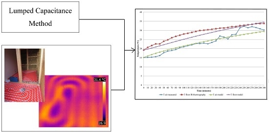
The present study examines the transient heat transfer in a hydronic concrete radiant floor; the temperature field is analysed by means of an analytical model and experiments in a test room. The calculated values of the floor temperature are then compared with values derived from an infrared thermography measurements campaign. The thermographic technique allows the retrieval of a wide thermal field on the floor surface without using a significant number of temperature probes. At the aim of enhancing the technique accuracy, the surface emissivity, the reflected temperature and the environmental thermohygrometric conditions have to be retrieved. With the support of a quantitative thermographic procedure in a large and significant portion of the floor, the study aims at verifying the applicability (and the limits) of the lumped capacitance model as an easy tool to analyse the thermal transient behaviour of a complex system composed by multi-layers stratigraphy and internal heat generation.

2. Experimental Test Rooms and Sensors

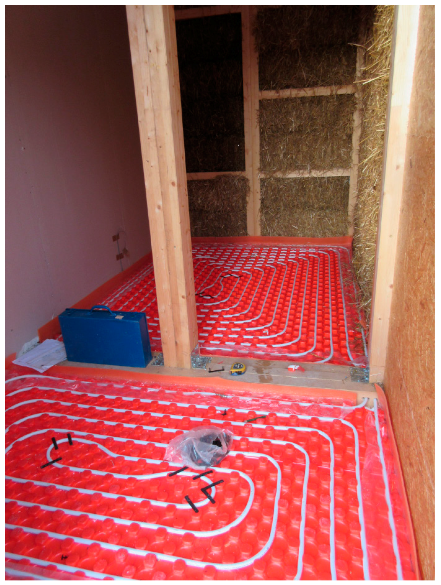
The monitored building is realized with a wooden structure, the external walls were made with 50-centimeters (cm) thick straw bales and the gable roof is closed with wood; the interior walls are covered by 2 cm of plaster (Figure 1). The room is 2.10 m wide and 4.32 m long; the maximum and minimum heights are respectively 3.00 m and 2.50 m. The test room presents an entrance facing the south-west direction; windows are not provided. The monitored chamber is equipped with a radiant floor, as shown in Figure 2; the system is insulated by an ashlar panel. The heat generator is an air to water heat pump.

The room floor structure is sketched in Figure 3: from the lower to the upper layer, the stratigraphy presents 30 mm thick wooden slab, 30 mm thick polystyrene panel, including the ashlar, the water pipe and 60 mm thick concrete screed. The pipes external diameter is equal to 16.3 mm and the internal one is equal to 12.5 mm.

The experimental set-up in the room is composed by two Tinytag surface temperature probes to measure the surface floor temperature, and two relative humidity and temperature Tinytag data loggers to monitor the thermohygrometric environmental conditions, both indoor and outdoor. Furthermore, a couple of water flow meters were mounted to monitor the two circuits mass flow rates. A series of thermocouples were positioned in the floor surface in order to set the emissivity of the floor for an accurate thermographic survey.

All the probes were connected by a personal computer with a data acquisition system.

An infrared (IR) thermal camera was used to carried out a thermographic analysis. The IR thermography analyses the thermal radiation emitted from an object. On the basis of the emissivity and the reflected temperature, the infrared thermal camera provides the surface temperature of the object. The portable IR camera is the B360 by FLIR model, with 320 × 240 pixels infrared resolution, 8–13 µm spectral range, temperature range from −20 °C to 120 °C, with thermal sensitivity of 0.05 °C at 30 °C [12]. It was installed on a tripod, at the centre of the room, positioned in a distance of 0.74 m to the floor, in order to better visualize the hot water circuit (Figure 4). At this distance between the lens and floor, the camera observed a region of 32 cm × 25 cm. The IR images (thermograms) were acquired each 10 min during the monitoring period.

The thermography technique revealed useful for the one shot evaluation of the floor thermal field. The lumped capacitance method describes the average temperature trend on the heating up phenomenon on the surface floor, therefore, the easier way to validate this calculation method is perfectly represented by the thermography survey, as it retrieves the entire superficial thermal field.

3. Analytical Model

The concrete layer is assumed to be subdivided in two regions: an upper region above the pipes and a lower region in to the pipe circuit above the insulation layer. The domain in which the model is applied belongs to the 4 cm thick upper region (Figure 3). The boundaries consist of two 10 cm × 10 cm surfaces (upper and bottom faces), chosen to match with a similar portion of the rectangular area viewed by the IR camera.

Hence, the mathematical model of the radiant floor heat transfer is applied to a domain constituted by a small volume of the concrete screed, paraellelepipedal shaped (0.10 m × 0.10 m × 0.04 m), with the upper face at the level of the floor surface.

The model is applied to a time interval between the instants t and (t + 1), and the procedure is repeated for the time steps t = 0,1,…,n−1, where n is equal to the number of divisions of the entire monitoring period. In each time step, the change of the screed internal energy is equal to the net heat transfer rate through the system boundaries, plus the rate of the energy generation within the system.

The heat transfer coefficient between air and solid takes account both the convection and irradiation heat. In addition, the test room is well insulated, thereby the temperature of the walls is close to the air temperature. For this reason, a constant heat transfer coefficient h is assumed during the transient period, representing the sum of the convective and radiant contributions:

$$h=h_c+h_r$$

(1)

where h_c and h_r are the heat transfer coefficients due to convection and irradiation heat, respectively.

Assuming constant properties of the concrete screed, the unsteady balance is described by the following equation:

$$\rho cV\frac{\partial T}{\partial t}=-hA(T(t)-T_{air}(t))+A\dot{q}$$

(2)

where ρ is the concrete density [kg/m³], c is the concrete specific heat [J/kg·K], V is the volume [m³], h is the surface heat transfer coefficient [W/m²·K], A is the upper surface of the domain [m²], $\dot{q}$ is the thermal power generated [W/m²] due to the heat transfer from the water pipes below the concrete screed. The heat flow density $\dot{q}$ is assumed to be as a known input, as it derives from design calculations, starting from the heat loads inside the room.

In the meantime, the overlying air is heated by the top surface of the screed and a heat exchange also occurs between air, walls and surroundings. Hence, the air temperature varies over time until reaching a constant temperature at steady-state conditions.

The room is so subdivided in paraellelepipedal control volumes with a base of 10 × 10 cm, and a height equal to the distance from the floor to the ceiling (2.75 m for the room under examination), including also its exterior layer (0.40 m, the thickness of the straw bale). The equivalent density and specific heat of each control volume are provided by the weighted average density ρ_r and specific heat c_r:

$${\rho }_r=\frac{{\rho }_a*V_a+{\rho }_c*V_c}{V_r}$$

(3)

$$c_r=\frac{c_a*V_a+c_c*V_c}{V_r}$$

(4)

where V_r is the entire volume of the room, V_a, ρ_a and c_a are referred to the volume, density and specific heat of air layer while and V_c, ρ_c and c_c are referred to the volume, density and specific heat of the straw bale ceiling.

The unsteady-state balance for each heating volume is defined by Equation (5):

$${\rho }_r{c}_r{V}_r\frac{\partial T_{air}}{\partial t}=hA(T(t)-T_{air}(t))+HS(T_{out}-T_{air})$$

(5)

where H is the heat transfer coefficent [W/m²·K], between the room and the external environment, including both heat transer by conduction and convection, calculated with the thermophysical properties of the wall materials. S is the exchange surface of the control volume, increased by the portion of the heat losses through thelateral walls of theroom.

The aforementioned parameters are summarized in

Table 1. Model input parameters.

Input Parameters	Value	Units
ρ	1200	kg/m3
c	840	J/kg·K
ρa	13.8	kg/m3
ca	1005	J/kg·K
ρc	100	kg/m3
cc	600	J/kg·K
A	0.01	m2
V	0.04	m3
h	10	W/m2·K
H	0.5	W/m2·K
q	75	W/m2

.

The relations (2) and (5) represent differential first-order equations, which aresolved with a numerical method, applying the finite difference method, in the temporal nodes (t, t + Δt), with t = 0,…, n−1 and time step Δt equal to 60 s:

$$\rho cV\frac{T(t+\mathrm{\Delta }t)-T(t)}{\mathrm{\Delta }t}=-hA\left[T(t)-T_{air}(t)\right]+A\dot{q}$$

(6)

$${\rho }_r{c}_r{V}_r\frac{T_{air}(t+\mathrm{\Delta }t)-T_{air}(t)}{\mathrm{\Delta }t}=hA\left[T(t)-T_{air}(t)\right]+HS(T_{out}-T_{air}(t))$$

(7)

Hence:

$$T(t+\mathrm{\Delta }t)=T(t)-\left[\frac{hA(T(t)-T_{air})+A\dot{q}}{\rho cV}\right]\mathrm{\Delta }t$$

(8)

$$T_{air}(t+\mathrm{\Delta }t)=T_{air}(t)-\left\{\frac{hA\left[T(t)-T_{air}(t)\right]+HS\left[T_{out}-T_{air}(t)\right]}{{\rho }_r{c}_r{V}_r}\right\}\mathrm{\Delta }t$$

(9)

Equations (8) and (9) allow the retrieval of the air and floor temperature during the transient period (T_air(t) ant T(t)). The floor heat transfer coefficient h is considered constant; in fact, its variation in the indoor environment results limited, since the air velocity is generally low and the surrounding objects temperature is not so different from the floor one.

4. Thermography Survey

In order to obtain an accurate quantitative thermography, some parameters were defined in the IR thermal camera software: the distance from the object, the emissivity, the air temperature, the air relative humidity and the reflected temperature. The distance of the lens from the object was measured; the emissivity was imposed with a comparison between the thermal camera readings and the temperature surface probes applied on the concrete. As mentioned previously, the air temperature and air relative humidity were measured by a Tinytag system and inserted in the thermal camera software. The aluminium foil method [13] has been used to evaluate the reflected temperature, which resulted close to the air temperature, because of the absence of significant heat sources. These parameters are reported in

Table 2. Parameters defined for the thermography survey.

Parameters	Value	Units
Distance of lens from the object	0.74	m
Emissivity	0.85	-
Air temperature	15.8	°C
Air relative humidity	49%	-
Reflected Temperature	16.0	°C

.

An area of around 10 × 10 cm has been drawn in order to evaluate the floor surface temperature in a portion of the thermogram. The average temperature on the surface from the pixel matrix of the area has been calculated each 10 min for each image acquisition.

The surface finish of the concrete screed allows to perform the thermography campaign reducing the “noisy” neighbouring surfaces reflection: this parameter could strong affect the IR analysis when the floor is covered by tiles. If this were the case, the use of insulating tape on the analysed surface to increase the emissivity and to decrease the reflection effects, should be taken into account. In the present study, the lack of tiles makes not necessary the use of the high emissivity tape.

In Figure 5 the time varying thermograms of the radiant floor system are shown, from the beginning of the campaign up to 300 min.

The water pipes are well distinguished in all thermograms, if the scale follows the floor heating, keeping constant the difference between the minimum and the maximum value (5 °C) of the entire picture. The temperature range inside the four squares analysed is equal respectively to 1.5, 1.4, 1.3 and 1.1 °C, showing that a more uniform temperature distribution is occurring as time goes on towards steady-state conditions, even if some spatial variations are still present after five hours of measurements.

The data elaboration of the IR images allows the trend definition of the surface temperature on the inspected floor during the five hours of acquisition, as for the average on the 10 × 10 cm portion shown in Figure 5.

5. Comparative Analysis of the Radiant Panels Transient

The values of the surface temperature obtained with the analytical model were compared with the average experimental data retrieved with the IR camera. A small area in correspondence of the water pipe was selected, experimentally investigated and analytically modelled. The chosen area was located close to the centre of the room.

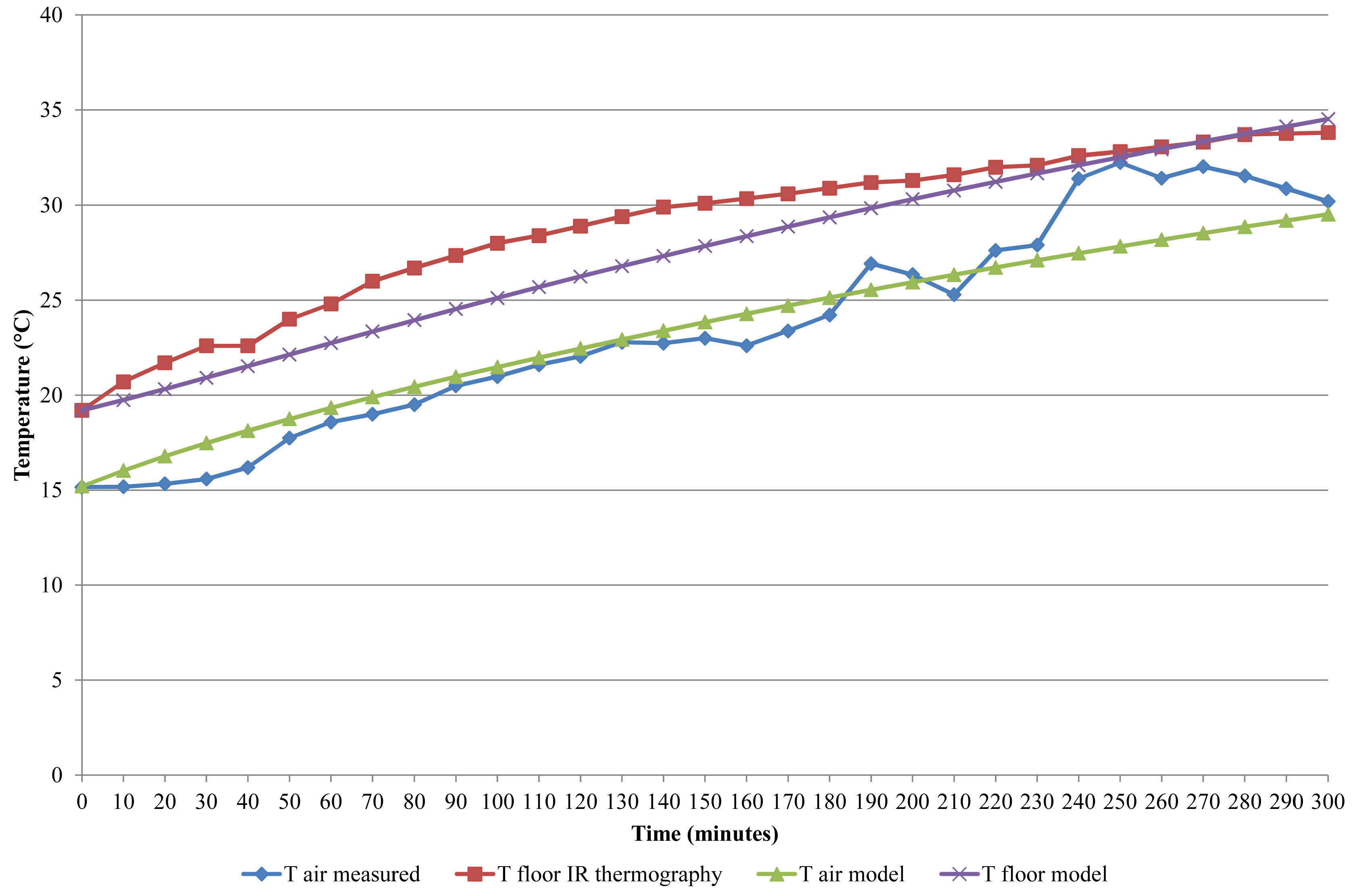
The floor temperature range varied from 19 °C to 34 °C during the overall monitoring period (300 min). The inlet water temperature was set to 43.0 °C.

Considering a time step of 10 min, the value predicted by the model was compared with the average temperature of the selected area of the IR image (Figure 6). During the start-up phase (0–200 min), the model seems underestimating the floor temperature raise, while the air temperatures result closer. On the contrary, at the end of the campaign (200–300 min), the measured and the modelled values of the floor surface temperature overlap, while the actual air temperature becomes higher, probably because of a sudden change of the external conditions (heat load by solar radiation, door opening, etc.), not included in the theoretical model.

In any case, the higher difference between the average thermographic data and the model retrieved temperatures result lower than 4 °C.

This slight difference between the two curves was expected, considering the simplifying assumptions of the semi-empirical model: the thermophysical properties of the materials constituting the floor (thermal conductivity, density and specific heat) were obtained by literature data;

–

the boundary conditions of the model are retrieved by measurements, which in turn are affected by a certain level of uncertainty;

–

the analytical model hypothesis of constant air temperature and constant heat transfer coefficient during the time interval, while these parameters are generally functions of time.

–

the heat flow $\dot{\mathrm{q}}$ is assumed to be constant;

–

the constant value assumed for the heat transfer coefficient H.

6. Conclusions

This paper presents an analytical and an experimental method aimed at describing the transient behaviour of a concrete radiant floor, made of a concrete screed, a layer of insulation below water pipes, an ashlar panel and a wooden slab.

A lumped capacitance approach was developed to analyse the floor temperature, hypothesizing a uniform temperature gradient of the concrete slab.

A radiant floor has been built in a test room to carried out experimental tests; with the purpose of better recreating the actual behaviour of the radiant floor, the boundary conditions of the analytical model were retrieved by field measurements.

The floor temperature distribution was assessed by an IR thermography analysis, which gave interesting information on the floor temperature distribution in a wide surface, as well as a comparative benchmark for the comparison with the analytical approach.

The values of the surface temperature obtained by the model were compared with the measured data, considering the same domain. The difference between calculated and measured values of the floor temperature remains lower than 4 °C throughout the entire monitoring period: a reasonable value if all the approximations of the analytical model and uncertainty of the thermographic measurements are taken into account.

Thus, once the design heat flow is known, as well as the outdoor temperature and the radiant floor and room envelope stratigraphy, the time-dependent air and floor temperature trend could be evaluated. The model and its IR measurements validation represent therefore a useful tool to understand at first sight the floor radiant panels behaviour in the start-up (and switch off) period, at the aim of gather useful information for the difficult task of their regulation.

The future work will be addressed towards the model validation in different and more numerous experimental environments; furthermore, the use of a computation fluid dynamics code for a three-dimensional representation of the domain could be implemented, obtaining, once validated by a similar experimental campaign, a more precise instrument for the radiant systems simulations.