
A Supervised Classification Method for Levee Slide Detection Using Complex Synthetic Aperture Radar Imagery


Abstract
:
1. Introduction
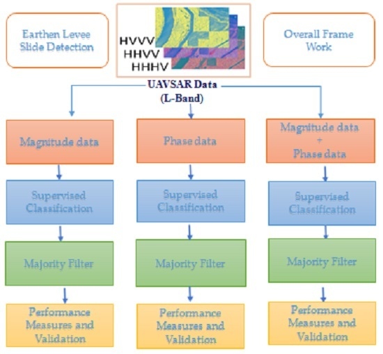
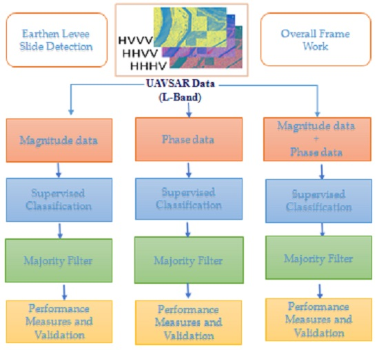
2. Method
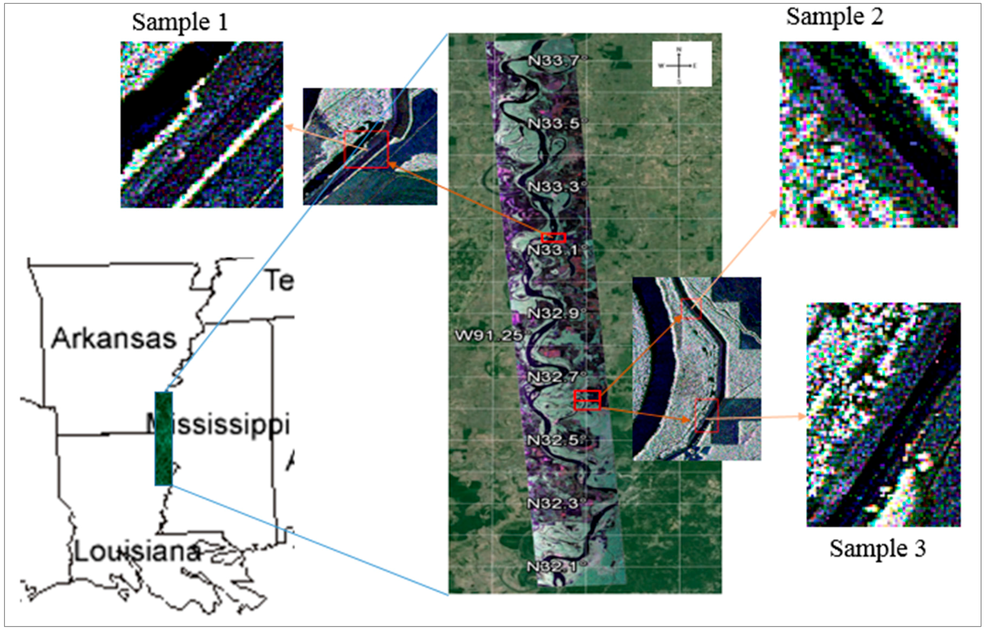
2.1. Data and Study Area
2.2. Training Data
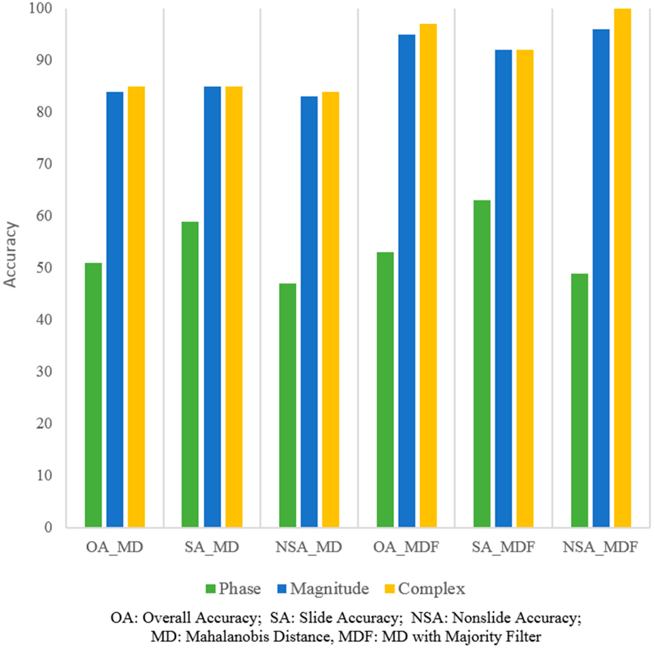
2.3. Mahalanobis Distance Classification
- D = Mahalanobis distance
- i = the ith class
- x = n-dimensional data (where n is the number of features)
- Σ−1 = the inverse of the covariance matrix of a class
- = mean vector of a class
3. Results and Discussion
4. Conclusions
Acknowledgments
Author Contributions
Conflicts of Interest
References
- Aanstoos, J.V.; Hasan, K.; O’Hara, C.G.; Prasad, S.; Dabbiru, L.; Mahrooghy, M.; Nobrega, R.; Lee, M.L.; Shrestha, B. Use of remote sensing to screen earthen levees. In Proceedings of the 39th Applied Imagery Pattern Recognition Workshop (AIPR), Washington, DC, USA, 13–15 October 2010; pp. 1–6.
- Dunbar, J. Lower Mississippi Valley Engineering Geology and Geomorphology Mapping; Program for Levees; US Army Corps of Engineers: Vicksburg, MS, USA, 16 April 2009. [Google Scholar]
- Hossain, A.K.M.A.; Easson, G.; Hasan, K. Detection of levee slides using commercially available remotely sensed data. Environ. Eng. Geosci. 2006, 12, 235–246. [Google Scholar] [CrossRef]
- Lin, S.W.; Ying, K.C.; Chen, S.C.; Lee, Z.J. Particle swarm optimization for parameter determination and feature selection of support vector machines. Expert Syst. Appl. 2008, 35, 1817–1824. [Google Scholar] [CrossRef]
- Ince, T.; Kiranyaz, S.; Gabbouj, M. Classification of Polarimetric SAR Images Using Evolutionary RBF Networks. In Proceedings of the 20th International Conference on Pattern Recognition, Istanbul, Turkey, 23–26 August 2010; pp. 4324–4327.
- Alvarez-Perez, J.L. Coherence, polarization, and statistical independence in cloude-pottier’s radar polarimetry. IEEE Trans. Geosci. Remote Sens. 2011, 49, 426–441. [Google Scholar] [CrossRef]
- Han, Y.; Shao, Y. Full Polarimetric SAR classification based on yamaguchi decomposition model and scattering parameters. In Proceedings of the 2010 IEEE International Conference on Progress in Informatics and Computing (PIC), Shanghai, China, 10–12 December 2010; pp. 1104–1108.
- Jong-Sen, L.; Pottier, E. Polarimetric Radar Imaging: From Basics to Applications, 1st ed.; CRC Press, Taylor & Francis Group: Boca Raton, FL, USA, 2009; ISBN 978-1420054972. [Google Scholar]
- Kong, J.A.; Schwartz, A.A.; Yueh, H.A.; Novak, L.M.; Shin, R.T. Identification of terrain cover using the optimal polarimetric classifier. J. Electromagnet. Waves Applicat. 1988, 2, 171–194. [Google Scholar]
- Lee, J.S.; Grunes, M.R. Classification of multi-look polarimetric SAR imagery based on complex Wishart distribution. Int. J. Remote Sens. 1994, 15, 2299–2311. [Google Scholar] [CrossRef]
- Lee, J.S.; Grunes, M.R.; Anisoworth, T.L.; Du, L.J.; Schuler, D.L.; Coulde, S.R. Unsupervised classification using polarimetric decomposition and the complex Whishart classifier. IEEE Trans. Geosci. Remote Sens. 1999, 35, 2249–2258. [Google Scholar]
- Cloude, S.R.; Pottier, E. An entropy based classification scheme for land applications of polarimetric SAR. IEEE Trans. Geosci. Remote Sens. 1997, 35, 68–78. [Google Scholar] [CrossRef]
- Aanstoos, J.V.; Dabbiru, L.; Gokaraju, B.; Hasan, K.; Lee, M.A.; Mahrooghy, M.; Nobrega, R.A.A.; O’Hara, C.G.; Prasad, S.; Shanker, A. Levee Assessment via Remote Sensing SERRI Projects; SERRI Report 80023–02; Southeast Region Research Initiative: Oak Ridge, TN, USA, 2012. [Google Scholar]
- Aanstoos, J.V.; Hasan, K.; O’Hara, C.; Dabbiru, L.; Mahrooghy, M.; Nobrega, R.A.A.; Lee, M.M. Detection of Slump Slides on Earthen Levees Using Polarimetric SAR Imagery. In Proceedings of the 2012 IEEE Applied Imagery Pattern Recognition Workshop, Washington, DC, USA, 9–11 October 2012.
- Exelis Visual Information Solutions User Guides and Tutorials. ENVI Version 5.1. Available online: http://www.exelisvis.com/Learn/Resources/Tutorials.aspx (accessed on 8 September 2016).
- Richards, J.A. Remote Sensing Digital Image Analysis; Springer-Verlag: Berlin, Germany, 1999; p. 240. [Google Scholar]
- Al-Ahmadi, F.S.; Hames, A.S. Comparison of four classification methods to extract land use and land cover from raw satellite images for some remote arid areas, Kingdom of Saudi Arabia. Earth Sci. 2009, 20, 167–191. [Google Scholar] [CrossRef]
- Canty, M.J. Image Analysis, Classification and Change Detection in Remote Sensing: With Algorithms for ENVI/IDL and Python, 3rd ed.; CRC Press, Taylor & Francis Group: Boca Raton, FL, USA, 2014; pp. 1–576. ISBN 9781466570375-CAT#K16482. [Google Scholar]
- Pajares, G.; López-Martínez, C.; Sánchez-Lladó, F.J.; Molina, Í. Improving Wishart Classification of Polarimetric SAR Data Using the Hopfield Neural Network Optimization Approach. Remote Sens. 2012, 4, 3571–3595. [Google Scholar] [CrossRef]
- Sánchez-Lladó, F.J.; Pajares, G.; López-Martínez, C. Improving the Wishart synthetic aperture radar image classifications through deterministic simulated annealing. ISPRS J. Photogram. Remote Sens. 2011, 66, 845–857. [Google Scholar] [CrossRef]


| Slide Number | Length | Vert. Face | Dist. from Crown | Latitude North | Longitude West | Date Slide Appeared | Date Slide Repaired |
|---|---|---|---|---|---|---|---|
| 1 | 135′ | 15′ | 12′ | N33-07′-44.4″ | W91-04′-46.1″ | October 2009 | March 2010 |
| 2 | 230′ | 7′ | 9′ | N32-37′-37.2″ | W90-59′-56.2″ | October 2009 | April 2010 |
| 3 | 80′ | 2′ | 30′ | N32-36′-37.7″ | W90-59′-42.3″ | October 2009 | November 2009 |
| 4 | 120′ | 3′ | 15′ | N32-36′-32.0″ | W90-59′-46.3″ | August 2008 | November 2009 |
| 5 | 200′ | 8′ | 8′ | N32-36′-29.1″ | W90-59′-48.0″ | - | September 2010 |
| Slide No. | From Levee Board (8 April 2011) | From Visual Aerial Photo Inspection | ||
|---|---|---|---|---|
| Date Slide Appeared | Date Slide Repaired | NAIP 2009 (May–September) | NAIP 2010 (May–September) | |
| 1 | October 2009 | March 2010 | Not Visible (25 July) | Unrepaired (3 August) |
| 2 | October 2009 | April 2010 | Not Visible (25 July) | Unrepaired (22 June) |
| 3 | October 2009 | November 2009 | Not Visible (25 July) | Repaired (22 June) |
| 4 | August 2008 | November 2009 | Unrepaired (25 July) | Repaired (22 June) |
| 5 | - | September 2010 | Unrepaired (25 July) | Unrepaired (22 June) |
| Data Type | Classification | Producer Accuracy % | User Accuracy % | Overall Accuracy % | |
|---|---|---|---|---|---|
| Method | Class | ||||
| Magnitude Data | MD | slide1 | 66 | 58 | 78 |
| nonslide | 82 | 87 | |||
| MDF | slide1 | 75 | 78 | 87 | |
| nonslide | 92 | 91 | |||
| Phase Data | MD | slide1 | 52 | 43 | 69 |
| nonslide | 75 | 81 | |||
| MDF | slide1 | 47 | 46 | 71 | |
| nonslide | 79 | 80 | |||
| Complex Data | MD | slide1 | 72 | 61 | 80 |
| nonslide | 83 | 89 | |||
| MDF | slide1 | 81 | 95 | 93 | |
| nonslide | 98 | 93 | |||
| Data Type | Classification | Producer Accuracy % | User Accuracy % | Overall Accuracy % | |
|---|---|---|---|---|---|
| Method | Class | ||||
| Magnitude Data | MD | slide2 | 85 | 71 | 84 |
| nonslide | 83 | 92 | |||
| MDF | slide2 | 92 | 92 | 95 | |
| nonslide | 96 | 96 | |||
| Phase Data | MD | slide2 | 59 | 34 | 51 |
| nonslide | 47 | 71 | |||
| MDF | slide2 | 63 | 36 | 53 | |
| nonslide | 49 | 74 | |||
| Complex Data | MD | slide2 | 85 | 72 | 85 |
| nonslide | 84 | 92 | |||
| MDF | slide2 | 92 | 100 | 97 | |
| nonslide | 100 | 96 | |||
| Data Type | Classification | Producer Accuracy % | User Accuracy % | Overall Accuracy % | |
|---|---|---|---|---|---|
| Method | Class | ||||
| Magnitude Data | MD | slide5 | 85 | 93 | 90 |
| nonslide | 94 | 87 | |||
| MDF | slide5 | 94 | 100 | 97 | |
| nonslide | 100 | 95 | |||
| Phase Data | MD | slide5 | 60 | 71 | 69 |
| nonslide | 77 | 67 | |||
| MDF | Slide5 | 69 | 90 | 81 | |
| nonslide | 92 | 76 | |||
| Complex Data | MD | slide5 | 91 | 97 | 94 |
| nonslide | 97 | 92 | |||
| MDF | slide5 | 98 | 100 | 96 | |
| nonslide | 100 | 98 | |||
© 2016 by the authors; licensee MDPI, Basel, Switzerland. This article is an open access article distributed under the terms and conditions of the Creative Commons Attribution (CC-BY) license (http://creativecommons.org/licenses/by/4.0/).
Share and Cite
Marapareddy, R.; Aanstoos, J.V.; Younan, N.H. A Supervised Classification Method for Levee Slide Detection Using Complex Synthetic Aperture Radar Imagery. J. Imaging 2016, 2, 26. https://doi.org/10.3390/jimaging2030026
Marapareddy R, Aanstoos JV, Younan NH. A Supervised Classification Method for Levee Slide Detection Using Complex Synthetic Aperture Radar Imagery. Journal of Imaging. 2016; 2(3):26. https://doi.org/10.3390/jimaging2030026
Chicago/Turabian StyleMarapareddy, Ramakalavathi, James V. Aanstoos, and Nicolas H. Younan. 2016. "A Supervised Classification Method for Levee Slide Detection Using Complex Synthetic Aperture Radar Imagery" Journal of Imaging 2, no. 3: 26. https://doi.org/10.3390/jimaging2030026
APA StyleMarapareddy, R., Aanstoos, J. V., & Younan, N. H. (2016). A Supervised Classification Method for Levee Slide Detection Using Complex Synthetic Aperture Radar Imagery. Journal of Imaging, 2(3), 26. https://doi.org/10.3390/jimaging2030026