Abstract
This article develops algorithms for the characterization and the visualization of micro-scale features using a small number of sample points, with the goal of mitigating the measurement shortcomings, which are often destructive or time consuming. The popular measurement techniques that are used in imaging of micro-surfaces include the 3D stylus or interferometric profilometry and Scanning Electron Microscopy (SEM), where both could represent the micro-surface characteristics in terms of 3D dimensional topology and greyscale image, respectively. Such images could be highly dense; therefore, traditional image processing techniques might be computationally expensive. We implement the algorithms in several case studies to rapidly examine the microscopic features of micro-surface of Microelectromechanical System (MEMS), and then we validate the results using a popular greyscale image; i.e., “Lenna” image. The contributions of this research include: First, development of local and global algorithm based on modified Thin Plate Spline (TPS) model to reconstruct high resolution images of the micro-surface’s topography, and its derivatives using low resolution images. Second, development of a bending energy algorithm from our modified TPS model for filtering out image defects. Finally, development of a computationally efficient technique, referred to as Windowing, which combines TPS and Linear Sequential Estimation (LSE) methods, to enhance the visualization of images. The Windowing technique allows rapid image reconstruction based on the reduction of inverse problem.
1. Introduction
The measurement of Micro–Nano features requires specialized imaging tools such as optical microscopes, thermal cameras, Scanning Electron Microscopy (SEM), and contact and non-contact position sensors. SEM can image conductive and non-conductive surfaces at a range of magnification from Millimeter to Nano scale; however, imaging a large micro-surface at high resolution is time-consuming and often destructive or impractical. For example, it is possible to capture a full view of a 3D microelectromechanical (MEMS) structure, such as that in Figure 1a, using SEM at 130X magnification, but the image quality at the interface, including the electrical and mechanical interconnections between the two structures, is poor. Thus, a 597X magnification of a smaller area was captured to reveal the micron features details, as shown in Figure 1b. The problem becomes one of stitching multiple images into a single image. In addition, the one drawback of SEM images is they do not provide depth information [1]. Toward these challenges, one of our objectives is to develop automatic and piece-wise algorithms that can reconstruct and enhance image visualization at minimum cost function. The reconstruction of images usually involves the interpolation of a large number of intermediate pixels from a smaller number of control points, which represents a digital elevation model (DEM) with the elevation being a quantity that represents the attribute interest. Typically, control points are sample locations of a captured or sampled pixel quantity at known (x,y) coordinates. Such quantities might be the pixel intensity matrix of an image or the sampled elevations of a micro-surface. DEMs carry vital information about the feature topography, and can be used to characterize or visualize images using reconstruction, feature extraction, and filtering enhancement techniques [2,3,4]. There is no single technique that is suitable for all types of image enhancement. For example, low pass and median filtering techniques alone are not appropriate for high quality reconstruction of images because they deteriorate its high frequency components [5]. Therefore, researchers developed a wide range of techniques that target the image’s components such as Markov random field (MRF), wavelet decomposition, Gaussian filter, multi-quadratic bi-harmonic method, Shepard’s method, C−1-Function interpolation method, kernel-based modeling method, and Thin Plate Spline (TPS) method [6,7,8]. In the kernel-based method, a penalized likelihood of the projection data is used to reconstruct images from the estimated coefficient model. However, the method is challenging because the inverse problem is ill-posed and the resultant image is usually very noisy [8]. TPS algorithm is used in the representation of 3D object from 2D images. TPS requires no assumption to be made with respect to the distribution or the location of the DEM. This method has become popular in the medical imaging because the reduction of the registration from global into local allows the analysis of local changes of image [9,10]. While many researches showed the applications of TPS in the visualization of macroscopic objects, little information is known about its ability to characterize or visualize micro and nano structures. Towards this goal, we aim to expand upon the application of TPS algorithm for imagining of MEMS structures.
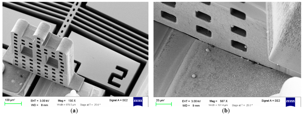
Figure 1.
Scaning electron microscopy (SEM) image of a 3D interconnected microelectricomechanical system (MEMS) structures: (a) the low magnification image shows the entire structure; and (b) the high magnification image shows the area of interest.
In Section 2, we derive mathematical models based on a modified TPS algorithm for the synthesis of the topological features of micro-surfaces. The interpolation algorithm is used to reconstruct images from few scattered data points. Then, we derive characterization algorithms to describe and extract image features in terms of topological slopes, curvatures, and bending components. We develop a Linear Sequential Estimation (LSE) based on TPS algorithm for a rapid reconstruction of images. Furthermore, we describe enhancement techniques to improve the image visualization, including image stitching, defect removal and resolution improvement. In Section 3, we conduct experiments to benchmark the performance of the proposed techniques. Finally, in Section 4, we demonstrate the algorithms using two illustrative examples: micro-surface of a MEMS based on a cloud of sampled points, and Lenna image.
2. Materials and Methods
2.1. Modified TPS Algorithm
The TPS is a non-stochastic algorithm that was first developed to minimize the bending energy of thin-plate structures. Such characteristic could be advantageous in smoothing the deformations due to large image pixilation or small micro-surface roughness [11,12]. This is because TPS has minimal bending energy properties over the entire object while it maintains the correlation with the DEMs [13]. The TPS algorithm uses radial basis function (RBFs), such as logarithmic RBFs and multi-quadratic function, which emphasizes on the local characteristics of the object, i.e., the reconstruction is largely unaffected at locations far from the RBFs. There is no unique procedure to define the RBFs; therefore, several basis functions have been developed and used in attempt to reconstruct objects from the measured DEMs [6,10,14].
In this research, we want to obtain a continuous, smooth, and differentiable model of an image or micro-surface that passes through its DEM. DEMs can be constructed with different patterns of data points as shown in Figure 2, depending on the target micro-surface, collection procedures and techniques employed. Toward this goal, we utilize the bi-harmonic partial differential equation of a thin plate under point loading [4,14,15]. We write
where Equations (1) and (2) correspond to the logarithmic RBFs of and the boundary conditions, respectively. The radial distance is . is the height or the pixel intensity level which is measured at coordinate. as and Fs are the coefficients of a nominal plane and the weighting factors of micro-surface, respectively. is the elastic constant at the interpolated point. and D are the spring and rigidity constants, respectively.
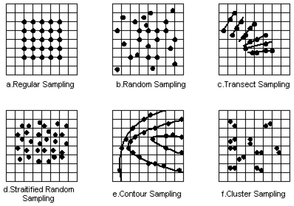
Figure 2.
Sampling patterns: DEMs distributed in x and y plane.
The interpolation function is divided into two parts [12]: (1) a linear part , and (2) the sum of the independent principal warp In this form, the logarithmic function is not defined when value is zero. Therefore, we add a small dimensionless quantity ε relative to to guarantee that Equation (1) is continuously differentiable function. This yields a modified TPS algorithm.
The above equation suggests that interpolated area could be either sharpened when ε is large or smoothen if it is small. The as’ and Fs’ coefficients in the boundary Equation (2) are unknowns, and they can be estimated by using DEM. We describe DEM by any arbitrary N control points whose Cartesian locations and magnitude values are known. We can write an N system of linear equations by substituting the DEM in Equation (3). The boundary conditions provide an additional three linear equations. The system of linear equations can be written in matrix form
where we define the TPS coefficient vector X by
and the measurement vector
The measurement model matrix H becomes
where H is . The distance between any two points can be measured relative to each other in any order. Therefore, H is symmetric matrix where . The inverse of H always exists except at singularity, which is either caused by dependent measurements, i.e., replication, or if the H matrix is constructed from three collinear samples. Therefore, if H is a positive definite and symmetric matrix, then we can estimate the coefficient vector from
The estimation algorithmic Equation (3) becomes a continuous and differentiable model whose coefficients are found from the information that is measured for the micro-surface.
2.2. Characterization of MEMS Micro-Surfaces by Using Modified TPS Algorithm
There are two popular types of bi-dimensional (2D to 2D ½) representations of microscale surfaces: SEM, and micro-surface profilometery. SEM produces an image of a sample by scanning it with a focused beam of electrons that contains information about the sample’s micro-surface topology. The produced image contains information about the planner dimension of the micro-surface, , but it does not directly provide depth information. The micro-surface profilometery approach uses contact or non-contact micron measurement sensing instrumentation, which is coordinated in a multi-axis micro-resolution motion stage. The produced image is typically a 2D ½ micro-surface constructed form a cloud of points of . For each of them, the same image-based analysis can be performed [16]. MEMS micro-surfaces exhibit topographical components that range from Nano, to Micro, to Meso scale size. The non-stationary and the multi-scale nature of a MEMS micro-surface could limit its description, which is typically provided by majority of the topographical characterization method employed [5,15,17]. Such micro-surface characterization algorithms tend to provide parameterized functions that are strongly scale dependent; however, one scale parameter cannot provide sufficient information about the micro-surface in all scales. This is because a scale parameter could conflict with multi-scale parameters as in the Permengham parameters that are used to describe 2D ½ micro-surfaces. These parameters were designed to characterize particular morphological features such as shape, elongation, shape complexity, and micro-surface directionality [18]. To overcome such shortcoming, we define the micro-surface characteristics of MEMS micro-surfaces by using the topological definitions that are commonly used in the description of geological landscapes; particularly, we obtain models from the derivatives of Equation (3) to characterize MEMS micro-surfaces. For example, the incremental change in micro-surface height as a point moves in lateral or horizontal directions is caused by a topography that contains peaks–hills–and valleys–dips. The angle switching between hills and valleys corresponds to changes in the continuity of micro-surface slopes. This corresponds to finding the slopes of a micro-surface in the x and y directions at the interpolated points; therefore, the slopes, and , are the first partial derivative of the reconstructed micro-surface in x and y at sample k, respectively.
The second partial derivative of the reconstructed micro-surface represents the slope variation of the micro-surface, or in the geological terms: the dip variation of the geological unit [6]. The micro-surface curvatures, and , in x, y and xy or yx are
We should point out that the second partial derivatives of the reconstructed micro-surface at the reconstructed points could be used for finite-element microstructural analysis [12].
The strike of a dipping layer is commonly used to describe the geological landscapes, and it is defined by the intersection of that layer with an imaginary horizontal plane; forming a line of equal elevations [7]. The strike is calculated by setting the x and y derivatives of Equation (3) to zero. This gives
This slope is the tangent of the angle between the positive x-axis and the strike line. The strike angle, δ, is the angle measured clockwise from the positive y-axis to the strike line, and it is a measure of the topographical contour slopes . The strike angle, estimated in degree, becomes
A vector, which is normal to the micro-surface at the reconstructed point, is defined by the azimuth, α, and the inclination—or dip angle θ in degrees. The direction of the true dip angle is always perpendicular to the strike; therefore, the azimuth measures the normality of a topographical micro-surface, and it is measured clockwise from the positive y-axis—or the north—such that the geological strike is equal to α + 90°. The azimuth is given by
By definition, dips at the reconstructed points depict positive inclination that is orthogonal to the strike line; therefore, the inclination or dip angle θ must be positive and is given by
The final characteristic that we obtain in this section describes the energy stored due to the deformations of micro-surface. The deformation index of a thin plate is subjected to slight bending, and it is derived for micro-surface based on the entire distributed bending energies, i.e., [19]. Applying this definition to Equations (11)–(13), we can define the following bending energy index at reconstructed point
The constant of proportionality, γ, has unit of J/m2 in the SI unit system. In addition, it is used as a qualitative scaling factor. The TPS function, z, in Equation (3) minimizes the nonnegative quantity of Iz; therefore, a planar micro-surface will have zero bending energy at areas where curvatures have high energy. A reconstructed topography of the bending energy is used as a qualitative measure of the geometry of a micro-surface at a location. For example, it views the negative features on a MEMS micro-surface image such as a micro-machined surface [15].
2.3. Image Processing Based on Modified TPS Algorithms
The classical image reconstruction techniques can be categorized into: intensity-based method, contour-based method, and shape-based method [20]. The intensity-based method requires information about the pixel intensity values and their locations within the image. We found previously that 2D ½ micro-surface can be reconstructed from cloud of points whose locations and height values are known in the Cartesian coordinate. It is possible to utilize TPS algorithm in the characterization and reconstruction of intensity-based images by replacing the z-value with intensity value. In this section, we will further develop techniques based on TPS algorithm for several image-processing enhancement, including denoising and rapid reconstruction.
2.3.1. Modified TPS Based Image-Reconstruction Method
The quality of an image tends to have better visualization when: (1) the image is reconstructed at high resolution; and (2) the original pixel intensity values of the image or the control points are inherited in the reconstructed image. Reconstruction of an image often involves the interpolation of regularly spaced intermediate pixels. Therefore, we select modified TPS with logarithmic RBFs algorithm, to interpolate the value of a new pixel within image region. Because the TPS coefficients in Equation (8) is solved by using the control points, the modified TPS algorithm, which is Equation (3), passes through these control points; therefore, the value of an interpolated pixel depends on the selected neighborhood that contains the control points. There are two types of neighborhoods:
- A spatial neighborhood: this technique reconstructs a region within an image by using the information that is available within it, and without the knowledge from other neighboring regions. The method can be applied either globally for the entire image, or locally for a selected region within the image.
- Spatio-to-temporal neighborhood: this technique reconstructs an image by sequentially updating the information from multiple neighborhoods. For example, an image could be reconstructed and warped from several regions.
2.3.2. Modified TPS Based Denoising Method
Image denoising is the process of filtering out impulsive defects, which typically requires algorithms for detection and removal of defects, and an algorithm that reconstruct the removed defects. Roman et al. [21] introduced a TPS method for denoising of old paintings with the additive noise modeled as random variable with zero-mean Gaussian distribution, and with the goal to achieve an acceptable trade-off between the noise removal and smoothing of edges. With the goal to decrease unwanted smoothing effect of TPS denoising, the proposed method by Roman uses a weighted TPS approximation of image data computed sequentially over small overlapping patches, and centered at each pixel. In this research, however, we describe procedures of a modified TPS image denoising that can: first, detect large defects, second recover lost information, and finally obtain a smooth reconstruction of the image. The method procedures is described as follow:
- Construct bending energy image, which is a greyscale intensity image of the defected image, and it is computed by using the bending energy index—Equation (18)—in the global coordinate. The impulsive defects are located in the constructed bending energy image because they are artifacts that tend to have black or white level with strong edges at their spatial boundaries [22]; therefore, a white pixel in the bending energy image corresponds to a black pixel in the original image, and it refers to a local maximum. A black pixel indicates a local minimum, and it corresponds to a white pixel in the original image.
- Obtain the locations of the defects from step (1), and then remove them to create a defect-free DEM; i.e., the original pixel intensity values are free of defect.
- Calculate the modified TPS coefficients from the updated DEM—from step (2)—by using Equation (8). There are two ways to calculate the modified TPS coefficients:
- Global: select all the available information from the updated DEM.
- Local: select a neighborhood for each defect.
- Interpolate the intensity value of the removed data by using Equation (3).
- If required, reconstruct high-resolution image by using the method described in Section 2.3.1.
2.3.3. LSE-TPS Based Warping Algorithm
In this section, we develop a LSE-TPS warping algorithm for the reconstruction of an image from multiple images. The goal is to warp multiple images into a single image, such as a torn image, while maintaining their spatial boundaries at the interface smooth. The spatial boundaries could be reconstructed at the same image resolution by using the method in Section 2.3.1, where a “good” warping would be dependent on a single neighborhood.
Our objective becomes to estimate the TPS coefficients from multiple neighborhoods; particularly we want to add weighting factors and directionality among neighborhoods. This way it becomes possible to emphasize on the reconstruction to selective neighborhoods. In this section, we refer neighborhood by a patch. Toward the end of this goal, we develop a LSE algorithm that updates the modified TPS coefficients between successive patches.
Suppose there is a L sequentially arranged patches. The application of LSE requires equal sizes of radial basis; i.e., each patch has n number of control points. Upon merging two successive patches—(k) and (k + 1) —into a single measurement model, we can write
This measurement model relates the states vector to the measurement matrix H, and the measurement error, , which is an additive Gaussian noise. In a static image, the s are set to zero; therefore, the H matrix becomes symmetric; where the elements in the main diagonal are equal to zero, and the TPS coefficient in B vector are not cross-correlated. The covariance of the measurement error is stationary in a single image, and it could be represented by a random diagonal variance matrix of zero means and known standard deviation. In snapshot imaging, such as SEM, the measurement errors and the process weight matrix, , are neither correlated forward nor backward in time. In addition, we assume that and are not cross correlated within an image i.e., .
Our goal is to minimize the propagation of the measurement errors when the estimated coefficients X are updated from one patch of data to another—window to window. We suggest that there exist an optimal coefficient vector X such that the Jacobin cost function, , is minimum; i.e.,
where the process weight matrix is diagonal, and it is given by
and corresponds to patches () and , respectively. The size of each process matrix is . The optimization of the Jacobian cost function with respect to produces minimum error. This is because the Hessian, which is the gradient of H, is positive definite; therefore, the optimization process can be written into the following covariance recursion process form
where Equations (23) and (25) are the information matrices, Equation (24) is the Kalman estimator gain matrix, and Equation (26) is the Kalman update Equation. These recursion equations estimate the TPS coefficient of patch by using its observation measurement and the modified TPS coefficient of patch ; therefore, a patch could be reconstructed based on its current information and the information available from the successive patch. The LSE-TPS method requires a-priori estimate of the coefficients. We can initialize the recursion process at k = 0 by
2.3.4. LSE-TPS Based Rapid Reconstruction Method
The solution of the radial basis functions requires matrix inversion, which could be problematic for large numbers of control points [6,7,19]. Equation (3) is dependent on the arithmetic operations that are required to compute the inverse of H; therefore, a large number of control points increases the number of computations. This mainly causes inaccuracy in the estimation of the modified TPS coefficient due to the accumulation of round-off errors. To improve the computational efficiency of the reconstruction and the visualization, we aim to reduce the size of the matrix H. Towards this goal, we develop the following Windowing technique:
Divide the image into L number of patches; each has equal number of control points. For example, Figure 3a contains 4-patches.
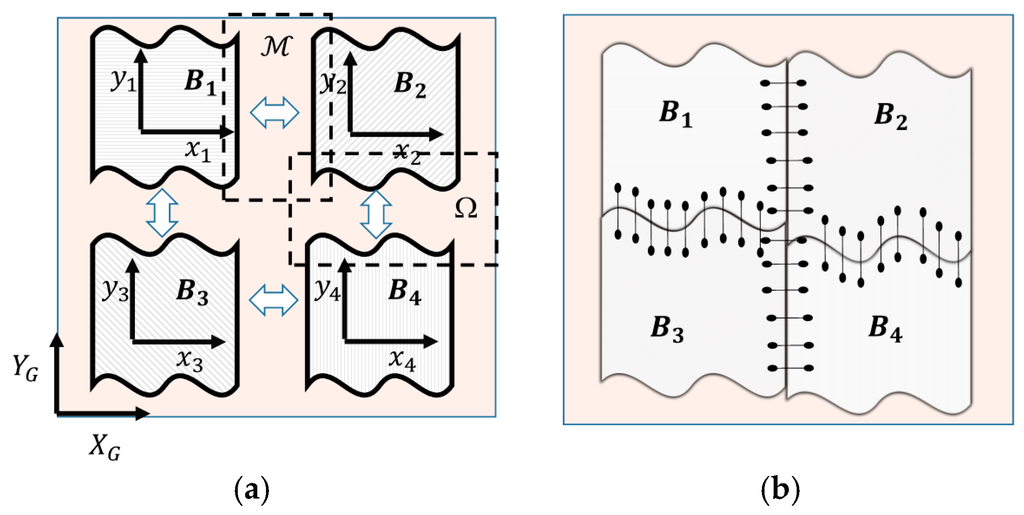
Figure 3.
Windowing technique in global and local coordinates: (a) Multiple patches; (b) Warping.
- Reconstruct each patch by using its own control points.
- Warp the patches at their spatial boundaries—for example, regions Ω and in Figure 3a—by selecting a neighboring set of control points for each boundary. Then, reconstruct the boundaries by using adequate method from Section 2.3.1, or the LSE-TPS algorithm that we described in Section 2.3.3. Figure 3b illustrate warping of multiple patches into a single image.
3. Discussion
In this section, we test the performance of the modified TPS algorithms and compare it with popular interpolation methods used in image processing.
3.1. Performance Studies of the Modified TPS and Windwoing Techniques
We study the perfromance of the Modified TPS for a grayscale image by evalauting its noise-to-signal ratio (SNR) and the accurcy of the interpolation algorithim, which is presented in Section 2.3.1. We define the accuracy by compairing the pixel value of the interpolated location with the true value of the pixel. To conduct such an experiment, we extracted a 100 × 100 Pixel2 image from Figure 1a, then reduced the resolution of the extracted image by half. This is done by removing the intermediate pixels from the 100 × 100 Pixel2 image. The results are shown in Figure 4.
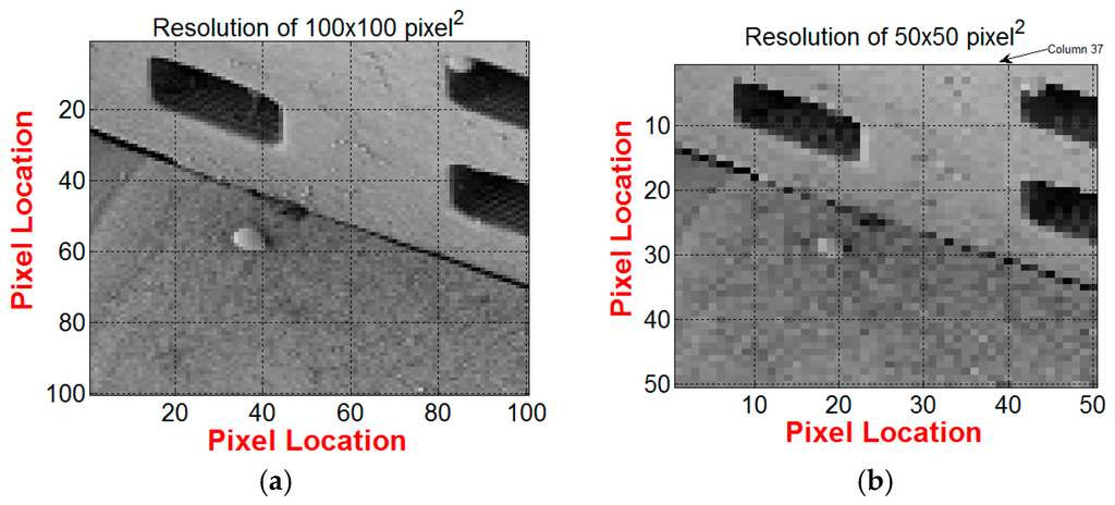
Figure 4.
Gray scale images extracted from SEM picture in Figure 1b: (a) Resolution is reduced down to 100 × 100 Pixel2; (b) Resolution is reduced down to Pixel2.
We use the global modified TPS method to double the resolution of the 50 × 50 Pixel2 image in Figure 4b. The pixel intensity is based on a grayscale image with a maximum intensity value of 256. The intermediate points, which bisect the mid distances between every two adjacent pixels in column 37 of Figure 4b, are interpolated using Equation (3).
We define the accumulative error between the true pixel value and the interpolated pixel at a location by
where is the number of samples, and the true values of vector are obtained from original image of 100 × 100 Pixel2 shown in Figure 4b. The total error based on the modified TPS with ɛ = 10−6 is calculated at column 37 and it is equal to 363.5187. It should be noted that the intermediate points suffer from small deviation from the true value as shown in Figure 5 and as noted by the non-zero values of accumulative error . The estimated value of a pixel at the DEM location is equal to the true value, i.e., coincident. This is shown in Figure 6, which plots three superimposed micro-surfaces in three dimension: (1) the triangulation of true pixel of image in Figure 4b; (2) the interpolation of the entire image whose pixels are evaluated at the location of each true pixel by using the Modified TPS method described in Section 2.3.1; and (3) the intermediate pixels which are interpolated along column 37.
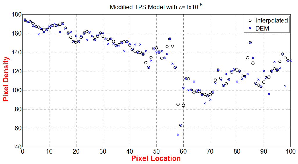
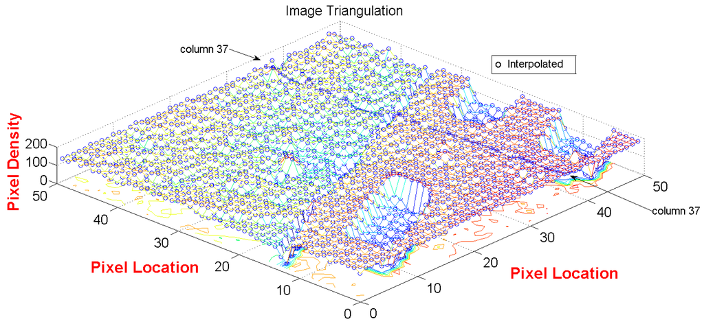
Figure 6.
Three dimensional micro-surface of the interpolated points superimposed on the true image surface.
The effect of correction factor ɛ in the accuracy of the modified TPS algorithm in grayscale image is studied for a range of values with results shown in Table 1. The method stays accurate for small values of ɛ whose values are comparable to the maximum pixel intensity value in grayscale image, but the method fails when ɛ becomes comparably large.

Table 1.
Effect of correction coefficient in the accuracy of the modified TPS method.
We utilize MATLAB built-in functions [23] to compare the accuracy of the Modified TPS with a few popular interpolation methods used in image processing toolbox. = interp2(, ‘Method’) function returns matrix containing elements corresponding to the elements of and and determined by interpolation within the two-dimensional function specified by matrices , , and . The methods that were tested are “nearest” or nearest neighbor interpolation, “linear” or Linear interpolation (default), “pline” or cubic spline interpolation, and “cubic” or cubic interpolation, as long as data is uniformly-spaced. Otherwise, this method is the same as “spline”. We use these methods to interpolate for the target values and then compare it with the modified TPS by using the cost function . The simulation results are summarized in Table 2, and show that the modified TPS is on average 770% more accurate than other listed methods.
Table 2.
Effect of correction factor in the accuracy of modified TPS method.
Another measure used to check on the quality of the interpolation method effectiveness is the relationship between SNR and the interpolation resolution. We designed a case study where a true image with 50 × 50 Pixel2 is used to reconstruct 100 × 100 Pixel2 image. The SNR values of the entire true images—50 × 50 Pixel2 and 100 × 100 Pixel2—are 14.9 and 15.1, respectively. Then, we compare the values of the SNR which is obtained for each method to reconstruct 100 × 100 Pixel2 image. Table 2 shows that the nearest method has the lowest SNR among other methods and it is sufficiently equal to the SNR for the true image of 50 × 50 Pixel2. This is due to the locality nature of the “nearest” method, which emphasizes the information available around the region of interpolated pixel. However, the modified TPS has the highest SNR value of 16.4 which could be explained by the global nature of the applied modified TPS method where all DEMs in the 50 × 50 Pixel2 is weighted in the interpolation.
The last performance measure of the modified TPS method is to understand how the SNR value varies with the number of the interpolated pixels in a given image. We use the source image of 50 × 50 Pixel2 in Figure 4b to increase the image resolution by using modified TPS method, and with ɛ = 10−6. The interpolation is carried out to interpolate the intermediate points between pixels, and with step up resolutions as indicated in Table 3. It can be concluded that the value of the calculated SNR increases as the resolution of the reconstructed image increase, however, to understand how such change is related to the size of the reconstructed image relative to the true image, we define SNR error percentage by . Where is the signal-noise ratio of the reconstructed image, and is the signal-noise-ratio of the true image used in the reconstruction. The simulation results in Figure 7 shows exponential convergence of β. i.e., the signal-to-noise ratio of a reconstructed image has maximum limit where it reaches saturation at certain pixel resolution. In this case study, the pixel resolution that corresponds to the saturation limit could be obtained from the following suggested fit-model: , where is the pixel intensity expressed by , and is a set of undetermined coefficients. The fit analysis is carried out by using MATLAB “fittool” GUI function. The coefficients are evaluated and found equal to . The “goodness of fit” is evaluated by using the regression coefficient, R2, which is equal to 0.9999. The final value of the fit-model, , can be found by using “limit theory”, and it gives , i.e., . The pixel intensity that corresponds to 1% within the range of the final value of is ~381 × 381 Pixel2. This explains that the SNR value of the reconstructed image would not change significantly at high resolution.
Table 3.
SNR relative to interpolation size in a modified TPS method.
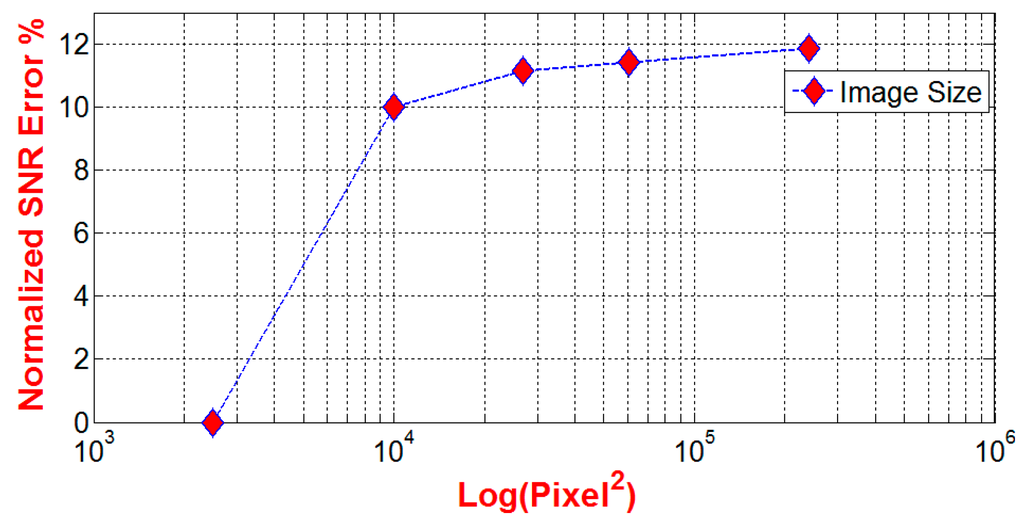
Figure 7.
Semi log plot of the SNR error percentage, β, and the size of the reconstructed image based on modified TPS method.
On the other hand, the computational efficiency of the windowing technique, which was discussed in Section 2.3.4, could be evaluated by comparing it with the global modified TPS method in terms of the number of computations required to invert H matrix. For example, the number of the computations required to invert H by using “Householder transformation algorithm” is 3/2n3 + O(n2) [24], where n is the total number of control points within an image. The Householder is a stable and efficient algorithm that is typically used for the inversion of large symmetrical matrices [25]; however, when an image is divided into L patches, the number of the computations becomes 3L/2(n/L)3 + O(n2); therefore, the number of the computation decreases when the number of patches increases. For example, suppose an image contains 1024 pixels. The number of computation required to inverse H matrix with L = 1 and L = 24 are 1.6 × 10⁹ and 2.8 × 10⁶, respectively.
3.2. Previous Studies
A comparison between the bending energy methods is compared with a few popular methods in Table 4. In addition, Table 5 provides a comparison between the developed reconstructions techniques with a few popular fundamental methods used in image restoration.
Table 4.
Comparison with methods used in edge detection.
Table 5.
Comparison with Fundamental methods used in image restoration.
4. Application Results
In this section, we implement techniques presented in Section 2 into two applications. Software codes were developed in this study by using MATLAB program [23].
4.1. Characterization of Micro-Surfaces Topology
We found in previous sections that the addition of a constant, ɛ, in the TPS model makes it possible to obtain contentious derivatives of the model in the spatial domain. Therefore, in this illustrative example, we characterize the topology of a micro-surface that contains roughness and waviness components. The height variation of a MEMS micro-surface in Figure 8a is measured at different location , and then it is registered in DEM. A 3D MEMS profiler, “Veeco” [37] is used to scan the micro-surface at spatial pixel resolution of 0.193 µm, and with a total number of control points of 479 × 639 Pixel2. Figure 8b shows a 3D visualization of the pad micro-surface plotted by using all the measured control points. The characterization of such data-rich model is computationally inefficient; therefore, a sufficiently small number of control points would be preferred.
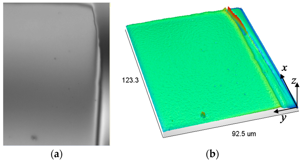
Figure 8.
Gold coated electrical-pad of a MEMS silicon micro-surface: (a) 50X optical image; (b) Triangulation of a measured micro-surface area of 92.5 μm × 123.3 μm.
A smaller data set of 10 × 10 Pixel2 is uniformly sampled from the DEM at a lateral pixel resolution of 0.965 µm. Figure 9a shows a linear triangulation of 100 control points covering an area of 92.5 µm × 123.3 μm. Equation (8) is applied to extract the TPS coefficients, and then the micro-surface is constructed at a smaller pixel size of 0.5 µm by using Equation (3). Figure 9b shows a continuous and smooth micro-surface that passes through all the 100 control points. The variation of the slopes in the x and y coordinates are obtained from Equations (9) and (10), and then they are plotted at 0.5 µm resolution, as shown in Figure 9c,d, respectively. Similarly, the curvature variation in the x and y coordinates are constructed by using Equations (11) and (12), with the results shown in Figure 9e,f, respectively. These later micro-surfaces measure the topography fluctuation; where a spiky point implies that there is a saddle point close to right angle. The strike angle in Equation (15) is a measure of the topographical contour slopes. Figure 9g shows a reconstruction of the strike micro-surface; i.e., non-uniform fluctuation of strike angles within ±90° range. The dips micro-surface in Figure 9h is constructed from Equation (17), and it shows positive inclination orthogonal to the strike line. The bending energy in Figure 9i is constructed from Equation (18), and it shows the bent variation in the micro-surface due to curvatures. The nodes, which are located on the infinite part of the extrapolated micro-surface, have negligible bending energies; therefore, the energy index can be used to detect the sudden changes within micro-surface such as holes, groves, and standing features in MEMS structures.
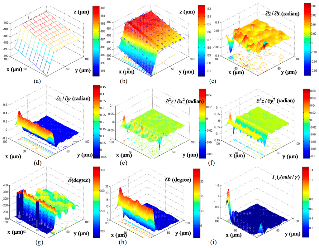
Figure 9.
Isometric views of: (a) Measured micro-surface; (b) Reconstructed micro-surface; (c) Interpolated slope micro-surface in x-direction; (d) Interpolated slope micro-surface in y-direction; (e) Interpolated curvature micro-surface in x-direction; (f) Interpolated y-direction curvature; (g) Interpolated micro-surface of strike angles; (h) Interpolated micro-surface of dip angles; (i) Interpolated bending energy micro-surface.
4.2. Visual Enhancement of Grayscale Lenna Image
SEM imaging suffers from the following shortcomings: (1) higher magnification leads to smaller field of view; therefore warping multiple images is needed for larger view; (2) high magnification often causes some damages to the specimen due to high electron field; therefore, there might be a need to filter out defects; and (3) high magnification could be non-feasible; therefore, there might be a need to reconstruct a higher resolution image from the lower magnification image. Because our algorithms can be applied to any greyscale SEM image, we select a standard picture from the image processing literature that is analogues to SEM images, and the goal is to guide the readers with the comparison. In this section, a noise-free Lena image [38], which is shown in Figure 10a, has a resolution of 512 × 512 Pixel2, and it is used to study the image processing techniques discussed in Section 4. A sub-image of 51 × 51 Pixel2 is extracted from the Lena image as shown in Figure 10b. This later image will be used throughout this section.
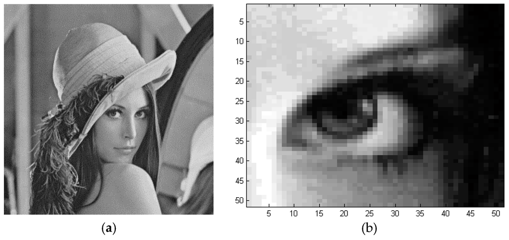
Figure 10.
Grey intensity image: (a) Lena Image; (b) A sub-image zoomed in the eye area of 51 × 51 pixels2.
The resolution of Figure 10b is reduced into a lower resolution image of 26 × 26 Pixel2 as shown in Figure 11a. The down sampling scheme followed here is conducted by removing the intermediate pixels located between every two adjacent columns and rows of the image in Figure 10b. The control points, which are contained in this low resolution image, is used to extract the TPS coefficients by using Equation (8), then a higher resolution image of 260 × 260 Pixel2 is reconstructed in the global coordinate by using Equation (3). The result is shown in Figure 11b.
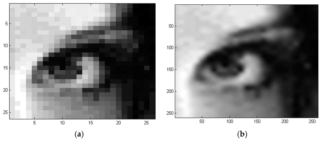
Figure 11.
Reconstruction from few control points by using global TPS algorithm: (a) Low resolution image containing 26 × 26 Pixels2; (b) Reconstructed at a higher resolution of 260 × 260 Pixels2.
An impulsive defect in the form of a black box is added to Figure 10b as shown in Figure 12a. The bending energy Equation (18) is applied to detect the edges of the defect. Figure 12b is the reconstructed bending energy image, and it shows the border of the defect cornered by white pixels; while the pixels away from defected area are registered black. We further implement the TPS methods to enhance the visualization of a defected image. A defect is added to a poor resolution image of 26 × 26 Pixel2 as shown in Figure 13a. The defect is detected by using the bending energy algorithm. The control points, which are corresponding to the defect, are removed from the image, leading to a DEM defect-free. This new DEM is used in Equation (3) to reconstruct a higher resolution image of 51 × 51 Pixel2 by using the global TPS algorithm, and the result is shown in Figure 13b.
Figure 12.
Detection of defects: (a) Defected image; (b) Defect detection by using the bending energy algorithm.
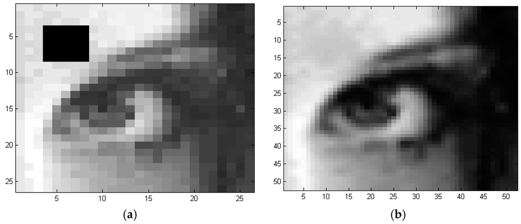
Figure 13.
Reconstruction of a poor image: (a) Defected and distorted image; (b) Automatic denoising and reconstruction.
We investigate the windowing techniques for a 51 × 51 Pixel2 image. Figure 14a is divided into 5 × 5 square windows. The modified TPS algorithm is then implemented at the local coordinates of each window with the goal to increase the overall image resolution. The overall image resolution has increased from 100 × 100 Pixel2 to 250 × 250 Pixel2 as shown in Figure 14b,c, respectively.
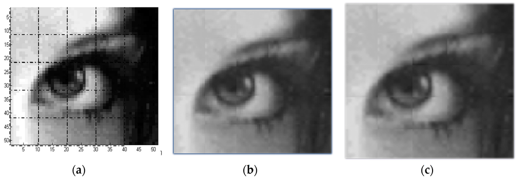
Figure 14.
Reconstruction by using local TPS method: (a) A 50 × 50 Pixel2 image is divided into 25 square windows; (b) Reconstructed image at resolution of 100 × 100 Pixel2; (c) Reconstructed image at resolution of 250 × 250 Pixel2.
A quick comparison between global and local modified TPS methods showed that the number of computations required to inverse H matrix of a 26 × 26 Pixel2 are 198, 977 and 37,500, respectively; however, the boundaries between the square windows are not smooth, and they become visually sharp when the resolution increases. This is observed in Figure 10b,c. To mitigate such shortcoming, the rest of this section studies the application of warping by using the procedures that we suggested in Section 2.3.3 and Section 2.3.4.
Figure 15a shows an image torn into four pieces, where the white area refers to the missing control points whose spatial locations (x,y) are known. The goal is to warp the pieces into a single image by using global modified TPS, local modified TPS and LSE-TPS methods. First, in the global modified TPS method, the missing pixels are evaluated by using the control points from all the four pieces together. The missing pixels are constructed at same image resolution, and the result is shown in Figure 15b. Second, the local TPS is used to warp the torn image in Figure 16a. The control points, which are located in the left or right part of the torn image, are used separately in the reconstruction of the missing pixels that are located in column 25. Figure 16b,c are reconstructed by using the information in the left part, and right parts, respectively.
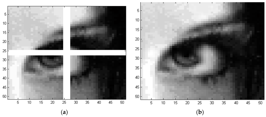
Figure 15.
Application of global TPS algorithm in warping images: (a) Torn image; (b) Warped image.
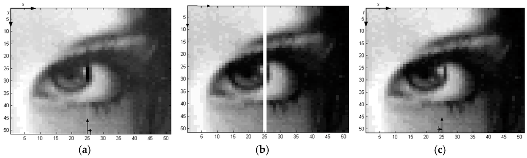
Figure 16.
Warping by using local TPS algorithm: (a) Torn image; (b) Reconstruction by using available information in the left part; (c) Reconstruction by using available information in the right part.
In the last warping method, we use the LSE-TPS to construct the missing column 25 by using the information from both column 24 and 26. In this method, the local TPS coefficients of each column 24 and 26 are computed separately. New TPS coefficients for column 25 are estimated from Equations (23)–(27), then column 25 is reconstructed by using Equation (3). The warping quality depends on the weighting matrix and the direction of propagation. For example, column 25 in Figure 17 is reconstructed by propagating the coefficients from left-right and right-left, respectively.
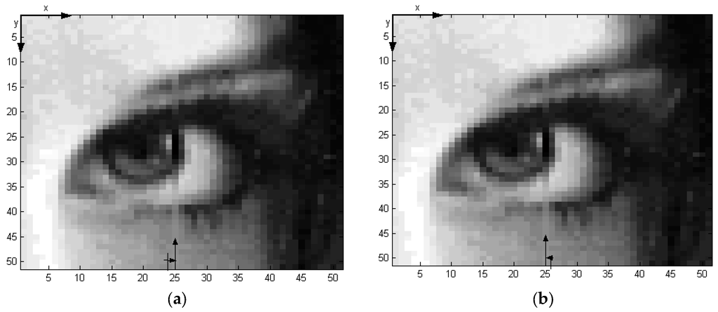
Figure 17.
Application of LSE-TPS algorithm: (a) Propagation from left to right; (b) Propagation from right to left.
5. Conclusions
In this research, we developed modified TPS and LSE techniques for the reconstruction and characterization of micro-surfaces and greyscale images. The techniques included: (1) reconstruction of an unknown micro-surface from a set of small data sample points; (2) restoration of bad samples; (3) filtering and warping of greyscale images; and (4) enhancement of micro-surface visualization and characterization of MEMS structures. Because the techniques are obtained from the modified ordinary TPS micro-surface, the source data, which is used to reconstruct micro-surfaces and images, are preserved. The reconstruction of high resolution images were conducted by using local or global logarithmic-based on modified TPS method. Local modified TPS restoration is dependent on a subset of data close to the point of evaluation; whereas a global method is dependent on all data. The benefit of global reconstruction of micro-surfaces is capitalized in its simplicity; however, the method is slow and inaccurate for large size of source data. On the other hand, we found that the windowing and warping techniques, when combined, could overcome the pitfall of the global method. Finally, we showed that the bending energy algorithm detects faults in a greyscale image, and locates bent micro-surface on MEMS structures.
Acknowledgments
This research is funded under professional grant from Bowling Green State University. The author would like to thank his collaborator Panos Shiakolas from the University of Texas at Arlington for valuable feedback.
Conflicts of Interest
The author declares no conflict of interest.
References
- Omrani, E.; Tafti, A.P.; Fathi, M.F.; Moghadam, A.D.; Rohatgi, P.; D’Souza, R.M.; Yu, Z. Tribological study in microscale using 3D SEM surface reconstruction. Tribol. Int. 2016, 103, 309–315. [Google Scholar] [CrossRef]
- O’Callaghan, J.F.; Mark, D.M. The extraction of drainage networks from digital elevation data. Comput. Vis. Graphics Image Process. 1984, 28, 323–344. [Google Scholar] [CrossRef]
- Zhang, L.; Zhou, R.; Zhou, L. Model reconstruction from cloud data. J. Mater. Process. Technol. 2003, 138, 494–498. [Google Scholar] [CrossRef]
- Kašpar, R.; Zitová, B. Weighted thin-plate spline image denoising. Pattern Recognit. 2003, 36, 3027–3030. [Google Scholar] [CrossRef]
- Mayyas, M.; Shiakolas, P.S. Micro-Surface Construction and Characterization From Digital Elevation Model Using Thin Plate Splines in Matlab Environment. In Proceedings of the ASME 2006 International Mechanical Engineering Congress and Exposition, Chicago, IL, USA, 5–10 November 2006; pp. 1105–1112.
- Algarni, D.A. Comparison of thin plate spline, polynomial, C I—Function and Shepard’s interpolation techniques with GPS-derived DEM. Int. J. Appl. Earth Obs. Geoinform. 2001, 3, 155–161. [Google Scholar] [CrossRef]
- Yu, Z. Surface interpolation from irregularly distributed points using surface splines, with Fortran program. Comput. Geosci. 2001, 27, 877–882. [Google Scholar] [CrossRef]
- Wang, G.; Qi, J. PET image reconstruction using kernel method. IEEE Trans. Med. Imaging 2015, 34, 61–71. [Google Scholar] [CrossRef] [PubMed]
- Raj, D.; Mamoria, P. Image Enhancement Techniques in the Spatial Domain: An Overview. IUP J. Comput. Sci. 2015, 9, 46. [Google Scholar]
- Gobbi, D.G.; Peters, T.M. Generalized 3D nonlinear transformations for medical imaging: An object-oriented implementation in VTK. Comput. Med. Imaging Graphics 2003, 27, 255–265. [Google Scholar] [CrossRef]
- Fornefett, M.; Rohr, K.; Stiehl, H.S. Radial basis functions with compact support for elastic registration of medical images. Image Vis. Comput. 2001, 19, 87–96. [Google Scholar] [CrossRef]
- Fornefett, M.; Rohr, K.; Stiehl, H.S. Elastic registration of medical images using radial basis functions with compact support. In Proceedings of the IEEE Computer Society Conference on Computer Vision and Pattern Recognition, Fort Collins, CO, USA, 23–25 June 1999.
- Barrodale, I.; Skea, D.; Berkley, M.; Kuwahara, R.; Poeckert, R. Warping digital images using thin plate splines. Pattern Recognit. 1993, 26, 375–376. [Google Scholar] [CrossRef]
- Lapeer, R.; Prager, R. 3D shape recovery of a newborn skull using thin-plate splines. Comput. Med. Imaging Graphics 2000, 24, 193–204. [Google Scholar] [CrossRef]
- Mayyas, M.; Shiakolas, P.S. Application of Thin Plate Splines for Surface Reverse Engineering and Compensation for Femtosecond Laser Micromachining. In Proceedings of the Intelligent Control, IEEE International Symposium on, Mediterrean Conference on Control and Automation, Limassol, Cyprus, 27–29 June 2005; pp. 125–130.
- Wejrzanowski, T.; Pielaszek, R.; Opalińska, A.; Matysiak, H.; Łojkowski, W.; Kurzydłowski, K. Quantitative methods for nanopowders characterization. Appl. Surf. Sci. 2006, 253, 204–208. [Google Scholar] [CrossRef]
- Mayyas, M.A.; Shiakolas, P.S. Microsurface Reverse Engineering and Compensation for Laser Micromachining. IEEE Trans. Autom. Sci. Eng. 2009, 6, 291–301. [Google Scholar] [CrossRef]
- Podsiadlo, P.; Stachowiak, G. Scale-invariant analysis of wear particle morphology—A preliminary study. Tribol. Int. 2000, 33, 289–295. [Google Scholar] [CrossRef]
- Joshi, A.A.; Shattuck, D.W.; Thompson, P.M.; Leahy, R.M. Registration of cortical surfaces using sulcal landmarks for group analysis of meg data. In International Congress Series; Elsevier: Amsterdam, The Netherlands, 2007; pp. 229–232. [Google Scholar]
- Joyeux, L.; Boukir, S.; Besserer, B.; Buisson, O. Reconstruction of degraded image sequences. Application to film restoration. Image Vision Comput. 2001, 19, 503–516. [Google Scholar] [CrossRef]
- Kaltenbacher, E.A.; Hardie, R.C. High-resolution infrared image reconstruction using multiple low-resolution aliased frames. In Proceedings of the Aerospace/Defense Sensing and Controls, Orlando, FL, USA, 8 April 1996; pp. 142–152.
- Bouzouba, K.; Radouane, L. Image identification and estimation using the maximum entropy principle. Pattern Recognit. Lett. 2000, 21, 691–700. [Google Scholar] [CrossRef]
- The MathWorks, Inc. MATLAB 8.5. Available online: www.mathworks.com (accessed on 14 September 2016).
- Businger, P.; Golub, G.H. Linear least squares solutions by Householder transformations. Numer. Math. 1965, 7, 269–276. [Google Scholar] [CrossRef]
- Chandrasekaran, S.; Gu, M. Fast and stable algorithms for banded plus semiseparable systems of linear equations. SIAM J. Matrix Anal. Appl. 2003, 25, 373–384. [Google Scholar] [CrossRef]
- Panchal, P.; Panchal, S.; Shah, S. A comparison of SIFT and SURF. Int. J. Innov. Res. Comput. Commun. Eng. 2013, 1, 323–327. [Google Scholar]
- Shah, U.; Mistry, D.; Patel, Y. Survey of Feature Points Detection and Matching using SURF, SIFT and PCA-SIFT. J. Emerg. Technol. Innov. Res. 2014, 1, 35–41. [Google Scholar]
- Harris, C.; Stephens, M. A combined corner and edge detector. In Proceedings of the Alvey Vision Conference, Manchester, UK, 31 August–2 September 1988; p. 50.
- Rezai-Rad, G.; Aghababaie, M. Comparison of SUSAN and sobel edge detection in MRI images for feature extraction. In Proceedings of the 2nd Internationl Conference on Information and Communication Technologies ICTTA’06, Damascus, Syria, 24–28 April 2006; pp. 1103–1107.
- Sobel, N.; Prabhakaran, V.; Desmond, J.; Glover, G.; Sullivan, E.; Gabrieli, J. A method for functional magnetic resonance imaging of olfaction. J. Neurosci. Methods 1997, 78, 115–123. [Google Scholar] [CrossRef]
- Pogue, B.W.; McBride, T.O.; Prewitt, J.; Österberg, U.L.; Paulsen, K.D. Spatially variant regularization improves diffuse optical tomography. Appl. Opt. 1999, 38, 2950–2961. [Google Scholar] [CrossRef] [PubMed]
- Natterer, F. Mathematical Methods in Image Reconstruction; Society of Industrial and Applied Mathematics (SIAM): Philadelphia, PA, USA, 2001. [Google Scholar]
- Franconi, L.; Jennison, C. Comparison of a genetic algorithm and simulated annealing in an application to statistical image reconstruction. Stat. Comput. 1997, 7, 193–207. [Google Scholar] [CrossRef]
- Zhou, Y.-T.; Chellappa, R.; Vaid, A.; Jenkins, B.K. Image restoration using a neural network. IEEE Trans. Acoust. Speech Signal Process. 1988, 36, 1141–1151. [Google Scholar] [CrossRef]
- Egmont-Petersen, M.; de Ridder, D.; Handels, H. Image processing with neural networks—A review. Pattern Recognit. 2002, 35, 2279–2301. [Google Scholar] [CrossRef]
- Wang, J.-H.; Liu, W.-J.; Lin, L.-D. Histogram-based fuzzy filter for image restoration. IEEE Trans. Syst. Man Cybern. B: Cybern. 2002, 32, 230–238. [Google Scholar] [CrossRef] [PubMed]
- Serry, F.; Stout, T.; Zecchino, M. 3D MEMS Metrology with Optical Profilers; Veeco Instruments Inc.: Tucson, AZ, USA, 2006. [Google Scholar]
- Wang, Z.; Bovik, A.C.; Evan, B. Blind measurement of blocking artifacts in images. In Proceedings of the International Conference on Image Processing, Vancouver, BC, Canada, 10–13 September 2000; pp. 981–984.
© 2016 by the author; licensee MDPI, Basel, Switzerland. This article is an open access article distributed under the terms and conditions of the Creative Commons Attribution (CC-BY) license (http://creativecommons.org/licenses/by/4.0/).