Article

Dense Descriptors for Optical Flow Estimation: A Comparative Study

1
Department of Electrical Engineering, University of Wisconsin-Milwaukee, Milwaukee, WI 53211, USA
2
Department of Mechanical Engineering, University of Wisconsin-Milwaukee, Milwaukee, WI 53211, USA
3
Departments of Computer Science and Electrical Engineering, University of Wisconsin-Milwaukee, Milwaukee, WI 53211, USA
*
Author to whom correspondence should be addressed.
J. Imaging 2017, 3(1), 12; https://doi.org/10.3390/jimaging3010012
Submission received: 17 October 2016 / Revised: 12 January 2017 / Accepted: 22 February 2017 / Published: 25 February 2017

Abstract

:
Estimating the displacements of intensity patterns between sequential frames is a very well-studied problem, which is usually referred to as optical flow estimation. The first assumption among many of the methods in the field is the brightness constancy during movements of pixels between frames. This assumption is proven to be not true in general, and therefore, the use of photometric invariant constraints has been studied in the past. One other solution can be sought by use of structural descriptors rather than pixels for estimating the optical flow. Unlike sparse feature detection/description techniques and since the problem of optical flow estimation tries to find a dense flow field, a dense structural representation of individual pixels and their neighbors is computed and then used for matching and optical flow estimation. Here, a comparative study is carried out by extending the framework of SIFT-flow to include more dense descriptors, and comprehensive comparisons are given. Overall, the work can be considered as a baseline for stimulating more interest in the use of dense descriptors for optical flow estimation.

1. Introduction

Optical flow estimation refers to the estimation of displacements of intensity patterns in image sequences [1,2]. Generally speaking, the problem can be formulated as a global energy optimization problem of the form E G l o b a l = E D a t a + λ E P r i o r where the data term, E D a t a , measures the point-wise similarity between the input images given the estimated optical flow and the prior term, E P r i o r , applies additional constraints for having a specific property for the flow field, for example smoothly varying flow fields. The choice of each term in the global energy functional and also the optimization algorithms varies in different methods for optical flow estimation.
As for the data term in the equation, one of the basic assumptions is to have constant brightness during movements of pixels. This assumption is the outcome of some other assumptions regarding the reflectance properties of the scene, the illumination and also the process of image formation in the camera [3,4]. These assumptions are not always true, and therefore, various methods are proposed to tackle the problems. Use of photometric invariant constraints, such as the constancy of the gradient in the work of Brox et al. [5], higher order derivatives proposed in [6] and color models with photometric invariant channels [7,8], have been investigated before. Another problem arises when having motion discontinuities and occlusions in the underlying flow filed, which can be remedied by the use of non-quadratic penalty functions for data terms and the smoothness term, as proposed by [9,10,11] and many other techniques in recent years.
Use of local/sparse feature detector/descriptors has been widely investigated in various branches of computer vision, namely wide baseline matching, object and texture recognition, image retrieval, robot localization, video data mining, image mosaicking and recognition of object categories [12,13,14,15,16,17,18,19,20]. In such techniques, the first step involves feature detection (corners, blobs, T-junctions, etc.). This is followed by assigning descriptor vectors to the neighborhood of each feature point and finally matching these descriptors between different scenes. Most of the descriptors can be divided into three major categories [21]: (1) distribution-based; (2) spatial-frequency; and (3) differential descriptors. In the first class, histograms are used for representing different characteristics of appearance and shape. Spin images [22] and scale-invariant feature transform (SIFT) [23] are two well-known examples of this class. Describing the frequency content of an image is used in the second class. Fourier transform represents image content by decomposing it into a linear combination of a set of basis functions. To have a more explicit spatial representation in the transformed image, Gabor filters [24] and wavelet transforms [25] are more suitable and are more used in the field of texture classification. In the third class, a set of image derivatives is computed in order to approximate a pixel’s neighborhood. Steerable filters [26] and complex filters [27,28] are two examples from this class.
Going towards more abstract problems like action recognition, pose or expression detection, object recognition/categorization, correspondence across different scenes, image retrieval, video classification and many more, local features/descriptors may not be the proper choice. In these cases, the need for dense descriptors is more suitable. Examples of this category can be found in [29,30,31,32,33]. However, there have been limited investigations on the use of feature descriptors for optical flow estimation [34,35,36].
Optical flow methods try to find a point-wise flow field between pixels of images in a sequence, and therefore, the use of descriptors in a dense manner can provide a good estimation. This is investigated in the work of Liu et al. [34] for the problem of dense correspondence across scenes by the use of dense SIFT descriptors. In their work, SIFT descriptors are computed for each individual pixel in the image, and then, by defining an energy functional constrained by data, small displacement and smoothness terms, dual-layer loopy belief propagation is utilized for optimization. The proposed technique is proven to be useful in video retrieval, motion prediction from a single image, image registration and face recognition. However, a more comprehensive evaluation of the method for optical flow estimation is missing. In this work, the main intent is to extend the proposed framework of SIFT-flow [34] to include more feature descriptors with additional analysis and investigations for optical flow estimation. For this purpose, for now, the use of seven texture descriptors in addition to SIFT is considered, and comprehensive analysis and comparisons with well-known datasets are provided. The used feature descriptors are: the Leung–Malik (LM) filter bank [37], the Gabor filter bank [24], the Schmid filter bank [38], the Root Filter Set (RFS) filters, steerable filters [26], Histogram of Oriented Gradients (HOG) [32] and Speeded Up Robust Features (SURF) [39].
The contributions of the current work can be summarized as follows:
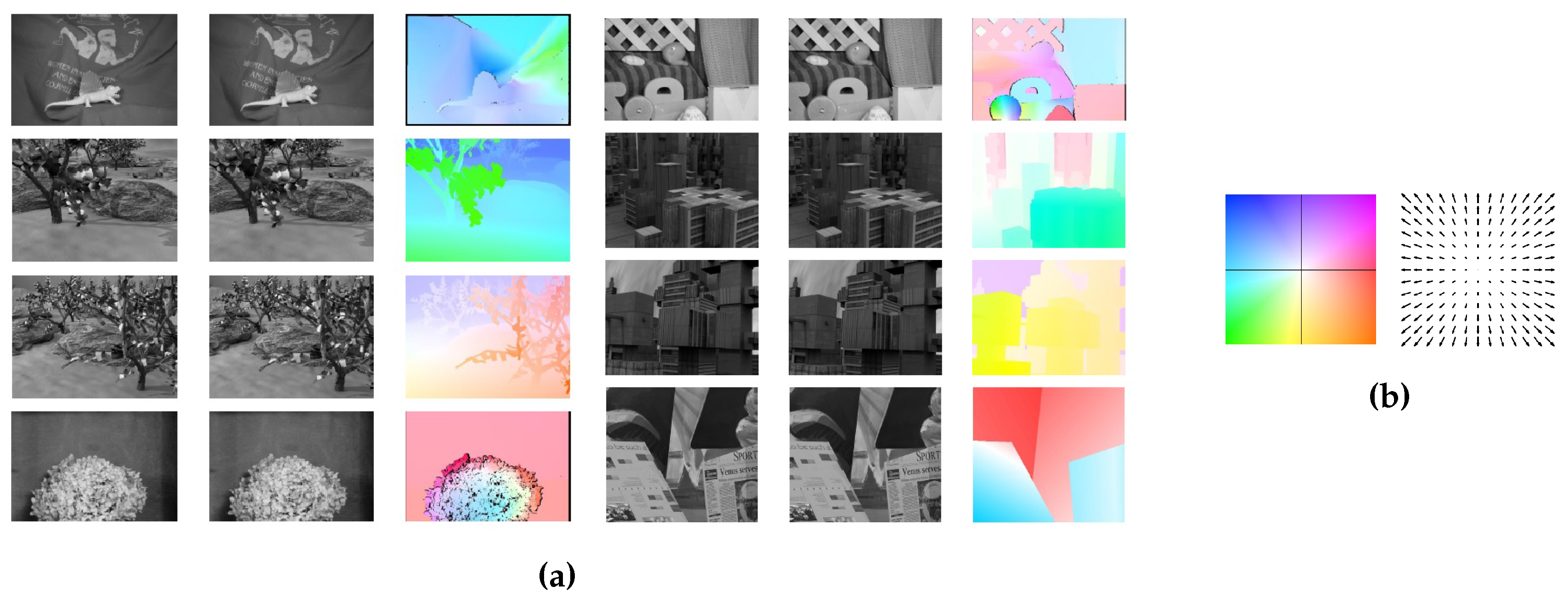
  • Given the framework proposed by Liu et al. [34], here, a comprehensive analysis is provided for the use of the framework for optical flow estimation. This is done by thorough comparisons using the widely-used Middlebury optical flow dataset [3]. This is to fill the gap in the original paper as no quantitative comparisons are given with the state-of-the-art in optical flow estimation.
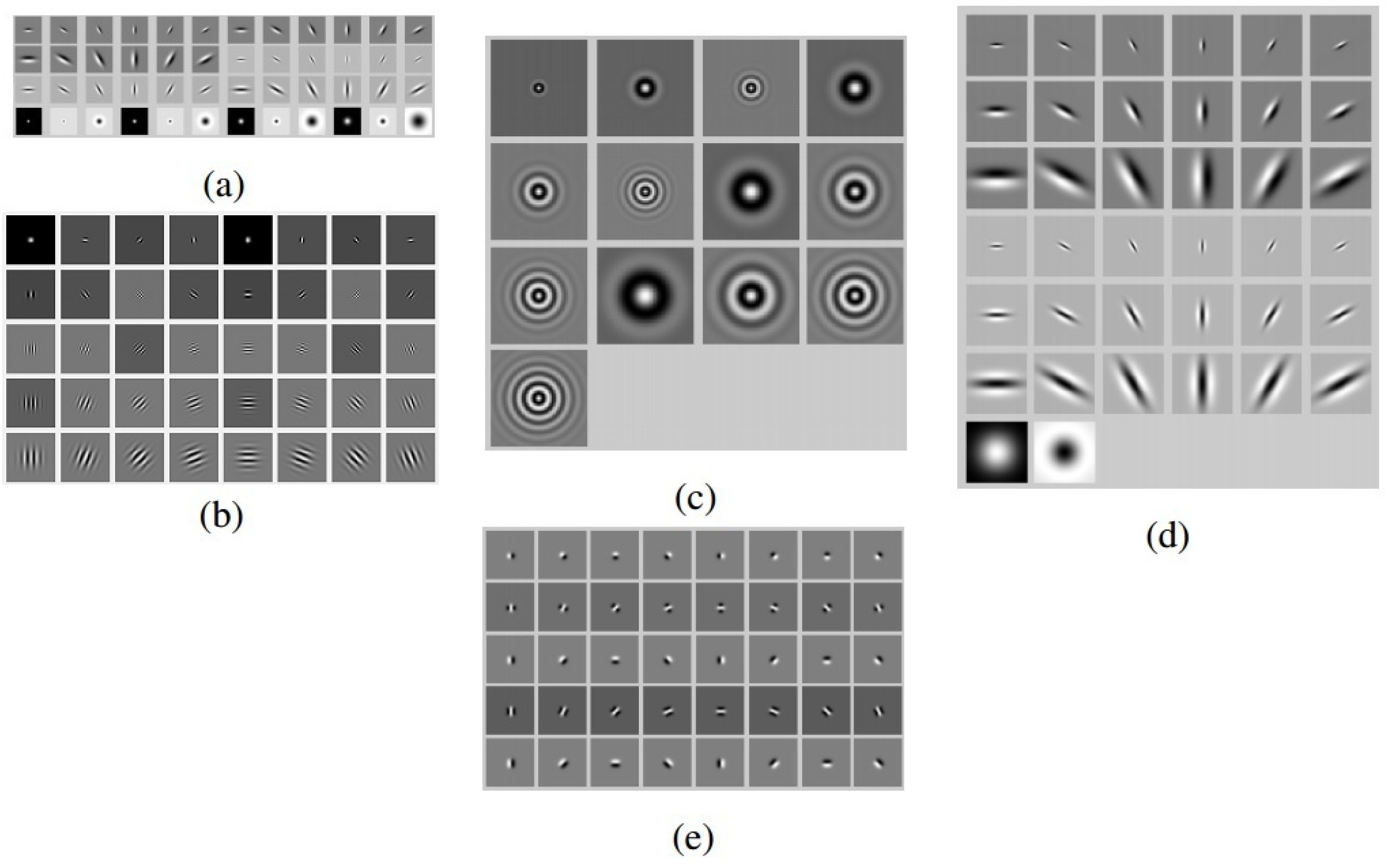
  • Aiming at extending the framework to include more dense descriptors, the use of a few other descriptors, namely the Leung–Malik (LM) filter bank, the Gabor filter bank, the Schmid filter bank, Root Filter Set (RFS) filters, steerable filters, Histogram of Oriented Gradients (HOG) and Speeded Up Robust Features (SURF), has been investigated and discussed for optical flow estimation.
  • To the best of our knowledge, this work is the first to utilize several of the proposed descriptors in a dense manner in the context of optical flow estimation. Therefore, we believe that this work will stimulate more interest in the field of computer vision for devising more rigorous algorithms based on the use of dense descriptors for optical flow estimation and dense correspondence.
One thing to note is that all of the images are converted to monochrome in this work, and therefore, the color is not utilized for optical flow estimation and dense correspondence. The rest of the paper is organized as follows: Section 2 contains a detailed explanation of the different descriptors. In Section 3, the general formulation of the framework is discussed, and the loopy belief propagation as the means for optimization is discussed in brief. Section 4 contains comprehensive comparisons of the used descriptors for optical flow estimation. It also contains pointers towards possible enhancements and future directions of the research. Finally, Section 5 concludes the paper.

2. Feature Descriptors

Feature detection and feature description are among the core components in many computer vision algorithms. Therefore, a wide plethora of approaches and techniques has been introduced in the past few decades to address the need for more robust and accurate feature detection/description. Even though there is no universal and exact definition of a feature that is independent of the specific application intended, methods of feature detection can be categorized into four major categories, as suggested by [40]: edge detectors, corner detectors, blob detectors and region detectors. The process of feature detection is usually followed by feature description, a set of algorithms for describing the neighborhood of the found features. As one can imagine, different approaches can be defined for describing features, which lead to various descriptor vectors. Generally speaking, the methods of feature description can also be classified into four major classes [40]: shape descriptors, color descriptors, texture descriptors and motion descriptors. By detecting the features and defining the descriptors, one can use the new representation of the input images for a wide range of applications, such as wide baseline matching, object and texture recognition, image retrieval, robot localization, video data mining, image mosaicking and recognition of object categories.
However, in some areas of computer vision, optical flow estimation or stereo matching for example, the outcome of an approach is required to be a dense flow field or depth map, respectively. Therefore, the use of sparse features is not suitable. In this case, by eliminating the first step of the process of feature detection/description, descriptors are defined for all of the pixels in the images. Of course, this requires significant changes in the process of feature matching with additional constraints in the optimization process. Here, the use of eight different texture descriptors is investigated and analyzed for optical flow estimation. In the following subsections, a detailed overview is given for each of the descriptors.

2.1. Gabor Filter Bank

Describing the frequency components of the images may also be considered in many applications. While Fourier transform decomposes the frequency components of an image into the basis functions, the spatial relations between the image pixels are not preserved in this representation [21]. Gabor filters, on the other hand, are designed to overcome this problem. The concept of Gabor filters is similar to that of wavelet transform. The difference is due to the fact that Gabor filters/basis functions are not orthogonal, and this may impose challenges in terms of computational complexity. However, Gabor features are widely used in many computer vision applications, such as texture segmentation and face detection. The general equation for the complex Gabor filter can be defined as follows [24,41]:
G ( x , y ) = s ( x , y ) w r ( x , y )
where s ( x , y ) represents a complex sinusoid defined as:
s ( x , y ) = e j ( 2 π ( u 0 x + v 0 y ) + P )
in which ( u 0 , v 0 ) is the spatial frequency and P is the phase of the sinusoid. As is obvious, this function has two components, one real and one imaginary. Therefore, the general Gabor filter also is composed of real and imaginary parts. The second term on the right-hand side, w r ( x , y ) , represents a Gaussian envelope, which can be defined as follows:
w r ( x , y ) = K e π ( a 2 ( x x 0 ) r 2 + b 2 ( y y 0 ) r 2 )
In the above equation, ( x 0 , y 0 ) represent the location of the peak, while a and b are scaling parameters, and the r subscript is for a rotation operation, which is represented by:
( x x 0 ) r = ( x x 0 ) c o s θ + ( y y 0 ) s i n θ ( y y 0 ) r = ( x x 0 ) s i n θ + ( y y 0 ) c o s θ
For this work, the efficient implementation of the Gabor filters in the frequency domain, elaborated in [42], is used. The number of filter frequencies and the number of orientations of the filters are set to 10 and eight respectively, which result in a set of 80 filters. Figure 1b shows a sample set of real-valued Gabor filters.

2.2. Schmid Filters

Schmid filters are a set of Gabor-like filters that combine frequency and scale with applications in texture classification and object recognition [38]. It should be noted that the basis elements of the Schmid filter bank are isotropic and rotationally invariant. The general form of such filters is as follows:
S ( x , y , τ , σ ) = S 0 ( τ , σ ) + c o s ( x 2 + y 2 π τ σ ) e x 2 + y 2 2 σ 2
in which τ is the number of cycles of the harmonic function within the Gaussian envelope of the filter, which is the same as the one used in Gabor filters. The term S 0 ( τ , σ ) is added for obtaining the zero DC component. This way, the filters are robust to illumination changes and invariant to intensity translations. Following the same approach as [38], 13 filters with scales σ between two and 10 and τ between one and four are used for creating dense descriptors. Figure 1c shows the set of Schmid filters used in this study.

2.3. Leung–Malik Filters

The main idea behind the set of LM filter bank comes from the concept of two-dimensional textons in which a texture is characterized by its responses to a set of orientation and spatial-frequency selective linear filters. This filter bank has a mixture of edge, bar and spot filters at multiple scales and orientations. The original set consists of 48 filters [37]; the first and second derivatives of the Gaussian at six orientations and three scales, which makes a total of 36 filters. It also includes eight Laplacian of Gaussian (LoG) filters, as well as four Gaussian filters. One version of the LM filter bank, named LM small, is composed of filters that occur at basic scales σ = { 1 , 2 , 2 , 2 2 } and first and second derivative filters that occur at the first three scales with an elongation factor of three ( σ x = σ , σ y = 3 σ x ). In this version, the Gaussians occur at the four basic scales, while the eight LoG filters occur at σ and 3 σ . In LM large, the filters occur at the basic scales σ = { 2 , 2 , 2 2 , 4 } . For the current work, the values of the parameters are set to their default values, which result in a set of 48 filters. Figure 1a shows the set of LM filters used in this study.

2.4. Root Filter Set Filters

The original Root Filter Set (RFS) consists of 38 filters, very similar to that of the LM filter bank. The filters are a Gaussian and a Laplacian of Gaussian, both with rotational symmetry and σ = 10 . This filter bank also includes edge filters at three scales ( σ x , σ y ) = { ( 1 , 3 ) , ( 2 , 6 ) , ( 4 , 12 ) } and bar filters at the same three scales. These two sets are oriented, which occur at six orientations at each scale. In the literature, RFS is usually used in a maximum response manner, in which only the maximum response for each orientation is considered [43]. This is mainly to achieve rotational invariance. However, in our implementation, the original set is used without considering the maximum response. The parameters of the filter bank are kept at their default values, which result in a set of 38 filters with size of 49 × 49 pixels and six orientations. Figure 1d shows the set of original RFS filters.

2.5. Steerable Filters

The idea behind the design of steerable filters comes form this question: What are the conditions for any function f ( x , y ) to be written as a linear sum of rotated versions of itself [26]? This can be represented as follows:
f ( x , y ) = j = 1 M k j ( θ ) f θ j ( x , y )
where M is the number of required terms and k j ( θ ) is the set of interpolation functions. In polar coordinates, r = x 2 + y 2 and ϕ = a r g ( x , y ) , and considering f as a function that can be expanded in a Fourier series in polar angle ϕ, we have:
f ( r , ϕ ) = n = N N a n ( r ) e i n ϕ
It has been proven that this holds if and only if the interpolation functions are solutions of:
[ e i n θ ] N × 1 = [ e i n θ m ] N × M [ k m ( θ ) ] M × 1
for n = 0 , 1 , 2 , N and m = 1 , 2 , , M . As stated and proven in [26], all band-limited functions in angular frequency are steerable, given enough basis filters. Steerable filters, 2D or 3D, are proven to be very useful in different fields of computer vision over the years [44,45]. Here, steerable filters of up to order five are used for creating dense descriptors. Odd orders are edge detectors, while even orders detect ridges. The number of orientations is set to eight. Figure 1e shows the set of steerable filters used here.

2.6. Histogram of Oriented Gradients

Histogram of Oriented Gradients (HOG) is based on computing a histogram of gradients in pre-determined directions [32,33]. The main idea comes from the observation that local object appearance and shape can usually be characterized by the distribution of local intensity gradients or edge directions. This can be implemented by dividing the image into small spatial regions, and for each region, a one-dimensional histogram of gradient directions or edge orientations is accumulated. To be more precise, at first, the gradient magnitudes in horizontal and vertical directions are computed, which results in a two-dimensional vector field for the image. In the second step, the magnitude of the gradient is quantized into several orientations. Then, these quantized descriptors are aggregated over blocks of pixels in the image domain. The next step is concatenating the responses of several adjacent pixel blocks, which is followed by normalizing the descriptors and sometime use of Principal Component Analysis (PCA) for reducing the dimensionality. Following the work of [33], Haar-features are used for calculating the gradient magnitude responses. To achieve the dense descriptors, the size of sub-blocks is set to 1 × 1 . Assuming a sectioning of 5 × 5 of the input images with the number of orientations equal to eight, the final dense descriptors are of a size of 200. Figure 2 shows a sample response of HOG on the Badafshan (the first author’s village in central part of Iran) image.

2.7. Speeded Up Robust Features

The Speeded Up Robust Features (SURF) method is designed to be scale and rotation invariant [39]. In SURF, features are detected using a Hessian detector, which in general consists of computing the convolution of a second order derivative Gaussian mask with the image in horizontal, vertical and diagonal directions for building the Hessian matrix for each pixel. Taking advantage of an approximation of these second order derivative Gaussian masks, the approximate determinant of the Hessian matrix can be computed very quickly. Moreover, the need for Gaussian smoothing and sub-sampling of the image for building the image pyramid can be eliminated by up-sampling these Haar-wavelet approximations and creating bigger masks for higher scales. Finally, the desired features are extracted by using a non-maximum suppression in a 3 × 3 × 3 neighborhood, followed by interpolating the maxima of the determinants of the Hessian matrices in scale and image space with the method proposed in the work of [46].
Since in this work, we are only interested in dense descriptors, there is no need for detecting the features within the image. However, still, the responses to the Haar-wavelets are needed. For defining the descriptor, at first, the orientation at each pixel is assigned. This is done by combining the results of applying the Haar-wavelets in a circular neighborhood around the interest point (or around each pixel, for defining dense descriptors). Next, a square region centered around the interest point and oriented along the estimated orientation is created, which is of the size 20 s , s being the scale. This region is further divided into smaller 4 × 4 sub-regions, each of the size 5 × 5 . With d x and d y as horizontal and vertical Haar-wavelet responses, respectively, a four-element vector is defined for each sub-region as V = ( d x , d y , | d x | , | d y | ) in which the summations are calculated over each sub-region. Having a vector of four for each of 16 sub-regions, a vector of size 64 is created as the descriptor of the pixel. For more detail on the different types of SURF, the reader is referred to [39].

2.8. Scale-Invariant Feature Transform

The four stages of Scale-invariant Feature Transform (SIFT) method are [23]: (1) scale-space extrema detection; (2) keypoint localization; (3) orientation assignment; and (4) keypoint descriptors. For the first step, a Gaussian function is considered as the scale-space kernel based on the work of [47]. By finding the scale-space extrema in the response of the image to Difference-of-Gaussian (DoG) masks, not only a good approximation for the scale-normalized Laplacian of Gaussian function is provided, but also as pointed out in the work of [48], the detected features are more stable. The local extrema of the response of the image to the DoG masks of different scales is found in a 3 × 3 × 3 neighborhood of the interest point. For accurate localization of the keypoints in the set of candidate keypoints, a 3D quadratic function is fitted to the local sample points. By applying a threshold on the value of this fitting function at the extremum, keypoints located in low contrast regions that are highly affected by noise are eliminated. Moreover, thresholding the ratio of principal curvatures can also eliminate poorly-defined feature points near the edges. After finalizing the keypoints, orientations can be assigned. This is done using the gradients computed in the first step of the algorithm when computing DoG responses. Creating a 36-bin histogram for orientations in the keypoint’s neighborhood is the next step. Each neighbor contributes to the histogram by a weight computed based on its gradient magnitude and also by a Gaussian weighted circular window around the keypoint.
The final step is creating the local image descriptor. Using the location, scale and orientation determined for each keypoint up until now, the local descriptor is created in a manner that makes it invariant to differences in illumination and viewpoint. This is done by combining the gradients at keypoint locations, as computed in the previous steps, weighted by a Gaussian function over each 4 × 4 sub-region in a 16 × 16 neighborhood around the keypoint into eight-bin histograms. This results in a 4 × 4 × 8 = 128 element vector for each keypoint. Normalizing the feature vectors to unit length will reduce the effect of linear illumination changes. This is usually followed by thresholding the normalized vector and re-normalizing it again to reduce the effects of large gradient magnitudes. Here, the descriptors are computed for all of the image pixels to create a dense descriptor for the image. For more information regarding the detail and implementation of SIFT, the reader is referred to [23]. Table 1 summarizes the number of dimensions of the various dense descriptors.

3. Methods

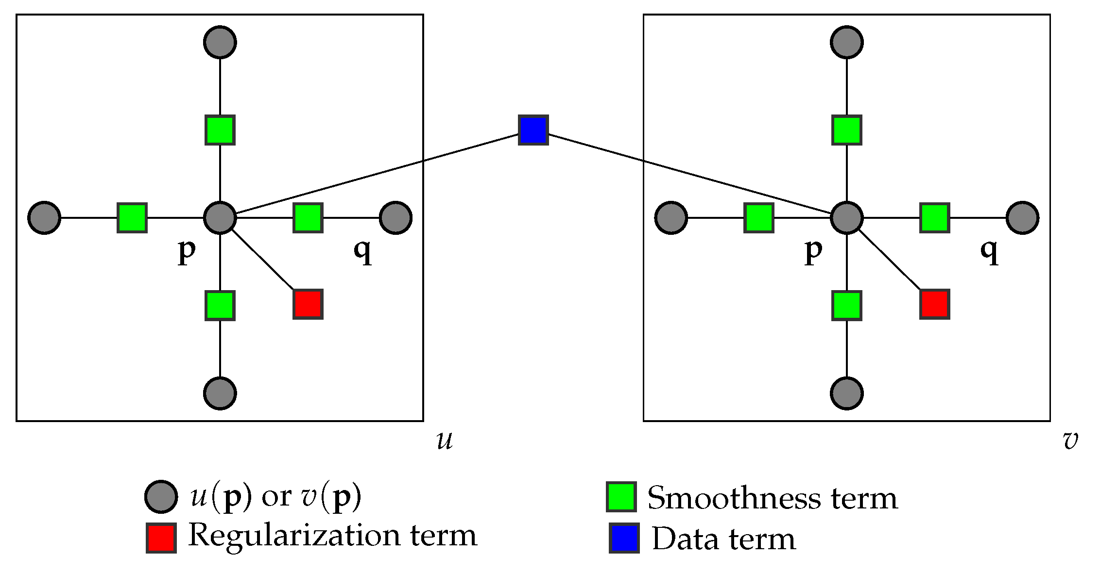
3.1. Problem Statement

The problem of matching/registering between images is modeled as a dual-layer factor graph, with de-coupled components for horizontal/vertical flow to account for sliding motion. This model is based on the work of [34], which takes advantage of the L 1 truncated norm for achieving higher speeds in matching. Assuming F 1 and F 2 as two dense multi-dimensional feature/descriptor images, which are created by using the descriptors explained before, and p = ( x , y ) as the grid coordinates of the image, the objective function to be minimized can be written as follows:
E ( w ) = p m i n ( | | F 1 ( p ) F 2 ( p + w ( p ) ) | | , t ) + p η ( | u ( p ) | + | v ( p ) | ) + ( p , q ) ϵ m i n ( α | u ( p ) u ( q ) | , d ) + m i n ( α | v ( p ) v ( q ) | , d )
in which w ( p ) = ( u ( p ) , v ( p ) ) is the flow vector at point p . The three summations in this equation are data, small displacement and smoothness terms, respectively. The data term is for minimizing the difference between the feature descriptors along the flow vector, while the small displacement term keeps the displacements as small as possible when no information is available. Finally, the smoothness term guaranties that the flow vectors for neighbor pixels are similar. A few parameters are used in this formulation. Here, t and d are data and smoothness thresholds and α and η are small displacement and smoothness coefficients, respectively. The values are set to the default values proposed by Liu et al. [34].
As is obvious, in this formulation, the horizontal and vertical components are de-coupled. This is mainly for reducing the computational complexity. However, this gives the additional benefit of being able to account for sliding motions during the procedure of image matching. The objective is considered as a factor graph, with ( p ) and ( q ) as the variable nodes, while the factor nodes represent the data, small displacement and smoothness terms. The flow is then extracted by using a dual-layer loopy belief propagation algorithm. Figure 3 shows the factor graph suggested by [34] for optimizing the energy functional of the dense matching problem. By using a coarse-to-fine (multi-resolution) matching scheme, one is able to reduce the computational complexity and hence the computation time while achieving lower values for the energy functional.

3.2. Belief Propagation

Belief Propagation (BP) is a technique for exact inference of marginal probabilities for single connected distributions [49]. Generally speaking, each node in the graph computes a belief based on the messages that it receives from its children and also from its parents. Such a technique, as may be obvious from the previous sentence, is purely local, which means that the updates are unaware of the global structure of the graph as the graph may contain loops and therefore be multiply connected [50]. In this case, BP cannot compute an exact solution, but at best an approximation, which can be surprisingly very accurate [49]. Use of graphical models in image processing tasks usually falls within the category of loopy graphs, which means different variants of BP are used and studied for solving different problems in this area [51].
In the general formulation of BP and subsequently Loopy BP (LBP) [52], we assume that node X computes its belief b ( x ) = P ( X = x | E ) , where E is the observed evidence that is computed by combining the messages from the node’s children λ Y j ( x ) and also its parents π X ( u k ) . Assuming λ X ( x ) as the node’s message to itself representing the evidence, we have:
b ( x ) = α λ ( x ) π ( x )
where:
λ ( t ) ( x ) = λ X ( x ) j λ Y j ( t ) ( x )
and:
π ( t ) ( x ) = u P ( X = x | U = u ) k π X ( t ) ( u k )
The message that X passes to its parent U i is given by:
λ x ( t + 1 ) ( u i ) = α x λ ( t ) ( x ) u k : k i P ( x | u ) k i π X ( t ) ( u k )
and the message that X sends to its child Y j is given by:
π Y j ( t + 1 ) ( x ) = α π ( t ) ( x ) λ X ( x ) k j λ Y k ( t ) ( x )
As is obvious from the equations, if a message is being generated to pass from node A to B, the contribution of the message from node B to A from the previous iteration is eliminated. Furthermore, normalizing messages at each iteration does not have any effect on the final beliefs and has the benefit of preventing numerical underflow [50].
Factor graphs are a means of unifying the directed and undirected graphical models with the same representation [53]. Such graphs are derived by the main assumption of representing complicated global functions of many variables by factorizing them as a product of several local functions of subsets of variables. Generally speaking, a factor graph can be defined as F = ( G , P ) in which G is the structure of the graph and P is the parameter of the graph. G , being a bipartite graph, can be defined as G = ( { X , F } , E ) where X and F are nodes variable and factor nodes, respectively, while E is a set of edges connecting a factor f i and a variable x X j . Given evidence as a set of variables with observed values, the process of belief propagation consists of passing local messages between nodes in order to compute the marginal of all nodes. Even though the same concept is used for belief propagation in directed graphs, here, the process can be formulated as passing messages between variable and factor nodes. In this case, two types of messages are passed: (1) message from the variable node to the factor node ( μ x f ) and (2) message the from factor node to the variable node ( μ f x ):
μ x f ( x ) h N x \ { f } μ h x ( x )
μ f x ( x ) N f \ { x } f ( X f ) y N f \ { x } μ y f ( y )
where x and y are variables, f and h are factors and N f and N x are representative of neighbors of the corresponding nodes in the graph. In acyclic graphs, the process of message passing is terminated after two messages are passed on every edge, one in each direction. In such graphs, the process results in an exact inference. Unlike acyclic graphs, belief propagation is done in an iterative manner in cyclic graphs. The process is terminated when having minimal changes in the passed messages according to a predetermined threshold, and the result is considered an approximate inference.
Several modifications to the general formulation of the energy minimization procedure are proposed by Liu et al. [34], which are also considered for this work. Different from the general formulation of optical flow, here, the smoothness term is decoupled for allowing separate horizontal and vertical flows. This reduces the computational complexity of the energy minimization significantly. In this implementation, at first, the intra-layer messages are updated for horizontal and vertical flows, and then, the inter-layer messages are updated between horizontal and vertical flows. Moreover, Sequential Belief Propagation (BP-S) [51] is used for better convergence. The reader is referred to the above-mentioned references for more detailed explanations and discussions on the subject.

3.3. Comparison Metrics

Assessing the performance of the proposed dense descriptors for optical flow estimation requires defining proper metrics for comparison. Here, three widely-accepted metrics for optical flow assessment are used [3].
Angular Error (AE), as the most commonly-used measure of performance for optical flow estimation, is defined based on the 3D angle between vectors ( u , v , 1.0 ) and ( u G T , v G T , 1.0 ) where ( u , v ) is the computed flow vector and ( u G T , v G T ) is the ground truth flow. AE can be computed by taking the dot product of the vectors divided by the product of their lengths as follows:
A E = c o s 1 ( 1.0 + u × u G T + v × v G T 1.0 + u 2 + v 2 1.0 + u G T 2 + v G T 2 )
Here, the Average of AE (AAE) over the image domain is used as one of the metrics.
Endpoint Error (EE), on the other hand, computes the absolute error between the estimated optical flow and the ground truth. This is to remedy some drawbacks associated with the AE. On the one hand, given the formulation of AE, errors in regions with smooth non-zero motion are penalized less than errors in regions of zero motion. Moreover, AE contains an arbitrary scaling constant (1.0) to convert the units from pixels to degrees. Given this, the EE can be defined as:
E E = ( u u G T ) 2 + ( v v G T ) 2
Here, the Average of EE (AEE) over the image domain is used as the metric.
Having two input images ( I 1 and I 2 ) as inputs of the optical flow estimation algorithm for computing the flow from I 1 to I 2 , it is possible to reconstruct an interpolated version of the second image by applying the computed dense flow to I 1 . This can be called I ^ 2 . The Interpolation Error (IE) can be defined based on the Root Mean Square (RMS) difference between the true I 2 and interpolated I ^ 2 using:
I E = 1 N x , y ( I 2 ( x , y ) I ^ 2 ( x , y ) ) 2
where N is the number of pixels.

4. Results and Discussion

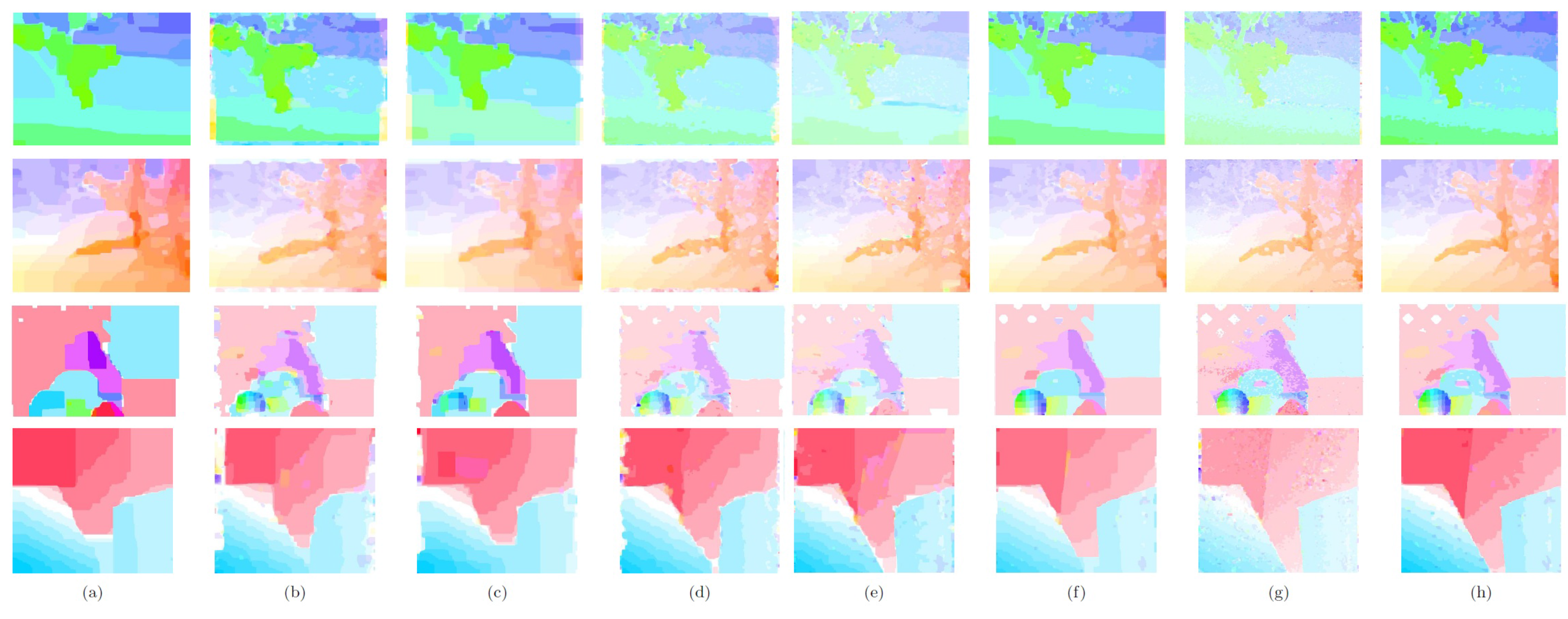
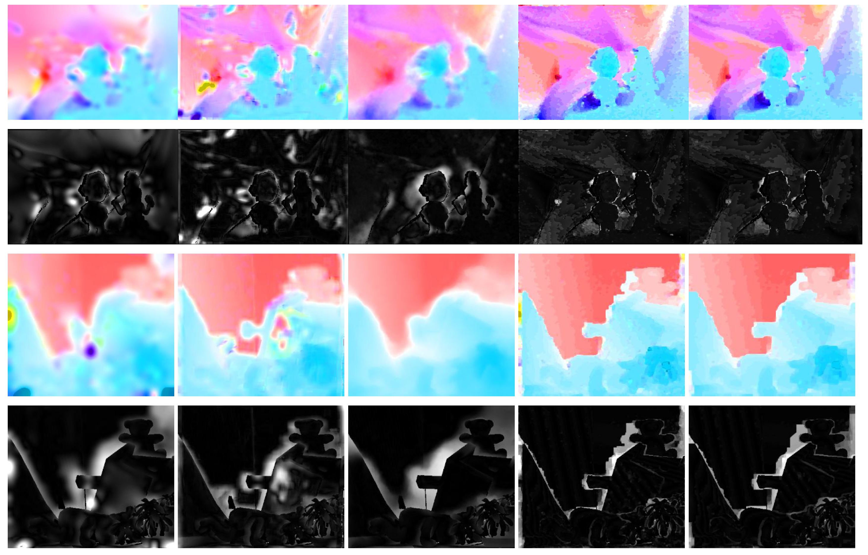
4.1. Evaluations and Discussions

Several widely-used databases are available on the web for assessing the performance of optical flow estimation algorithms [3,54]. Figure 4a shows the set of training pairs, as well as the optical flow’s ground truth used in this study acquired from the Middlebury optical flow database (http://vision.middlebury.edu/flow/). The set consists of eight pairs of monochrome images, namely Dimetrodon, Grove2, Grove3, Hydrangea, RubberWhale, Urban2, Urban3 and Venus, with the ground truth optical flow. Figure 4b shows the color map use for visualization of the flow fields.
Table 2 represents the comparison between the performance of different dense descriptors in terms of average angular error in comparison to the ground truth. Table 3, on the other hand, shows the results of comparison between the various dense descriptors in terms of endpoint error. The last column in the tables shows the average ranking of the different descriptors for estimating the optical flow on the training set. Inspecting the results, it is shown that dense SIFT is able to capture the structural representations of the objects contained in the sequences in a more robust and reliable way in comparison to the rest, while the performance of the dense Schmid descriptor is the worst. This is somewhat expected since the Schmid filter bank contains a set of isotropic filters in comparison to the rest of the descriptors that can capture the orientation of the edges and boundaries within frames. One important factor in determining the superiority of a descriptor is the ability to capture the structural representation of the scene in a multi-scale/multi-resolution manner. Even though this is the case for several of the descriptors as mentioned before in the previous sections, dense SURF and dense SIFT descriptors have superior performance to the rest. As mentioned before, SURF, as is obvious from its name, utilizes simplifying approximations to be able to speed-up the process of descriptor creation. In this method, second order derivatives of the Gaussian are approximated with binary Haar-wavelets. This approximation, even though appropriate in sparse feature description, causes granular patterns in the final optical flow estimations. The phenomenon can be seen more obviously in uniform regions of the flow fields, for example in Venus. Figure 5 shows the results of the dense descriptors for Grove2, Grove3, RubberWhale and Venus for visual comparison.
Table 4 represents the result of the dense descriptors in terms of interpolation error (IE). In order to eliminate the marginal errors, a margin of 20 pixels is considered for computing the IE. In terms of interpolation error, dense SURF is able to perform the best among other methods. This may seem strange that SIFT performs better in estimating the optical flow while SURF is able to provide a better reconstruction when warping the images. However, it should be noted that these two are not necessarily equivalent. This can be mainly attributed to the simplifying assumptions made during the generation of SURF features. As mentioned before, SURF uses binary Haar-wavelets in order to approximate the second order derivatives of Gaussian functions. While this is done to achieve higher computational speed, it can cause the optimization process of the energy functional to fall into local minima. This is evident from the estimated optical flow using dense SURF descriptors, as shown in Figure 5, where granular patterns can be seen in uniform regions. While this may reduce the interpolation error in these regions, the overall optical flow estimate can suffer from increased error. Of course, the difference is not very noticeable between the methods in terms of accuracy. It should be noted that in the examples that are presented here, illumination variation is not a factor when going from one frame to another. When we have variations in the intensity levels and lighting between sequential frames, the IE metric is not a reliable representatives of the performance, and only AE can determine the true error.
For the completeness of the comparisons, a few of the techniques from the Middlebury database are chosen here, namely Pyramid-LK [55], FOLKI [56], SLK [57], PGAM+ LK [58] and FFV1MT [59]. Since the performance of the dense SURF and dense SIFT are superior to the rest of the proposed dense descriptors, only these two are considered for comparison. Table 5 contains the results of the comparison between these various techniques with dense SIFT and dense SURF in terms of the average and standard deviation of the angular errors. In Table 6, the results of the comparison in terms of the average and standard deviation of the endpoint error is given. The last column in both tables shows the overall ranking of the methods in the Middlebury dataset. While the performance of the different methods varies when estimating optical flow between different images, the performance of dense SIFT is better in general. Figure 6 shows the resulted optical flow estimation from SLK, PGAM + LK, FFV1MT, dense SURF and dense SIFT alongside the error maps for the Mequon and Teddy image pairs. Unlike SLK, PGAM + LK and FFV1MT, which suffer from severe smoothing effects near edges and in regions with fine details, dense SURF and dense SIFT perform better, significantly.

4.2. Possible Enhancements and Future Directions

Careful investigation of the performance of the various dense descriptors reveals several possible directions for improvement. Especially when comparing the results of the methods with the state-of-the-art, they seem to perform poorly. However, it should be noted that studies on the use of dense descriptors for the problem of optical flow estimation are still very limited. Therefore, more research should be done in this area in order to achieve more robust and accurate techniques.

4.2.1. Parameter Optimization

Each of the above-mentioned descriptors requires a set of parameters to be specified for the optimal representation of image sets. The parameters include the support of filter banks, the spread of the kernel function, the number of orientations, etc. Depending on the images and the level of content in terms of size and resolution, setting the descriptors’ parameters properly may have a significant effect on the final computed flow field. An automatic and content-adaptive parameter setting can help to improve the performance of the methods significantly. Sharp edges, high velocities between frames and occlusions impose the most difficult challenges for optical flow estimation in general. Even though, overall, the dense descriptors are capable of estimating the flow, since there is no strategy for occlusion detection, this results in angular errors in the estimated flow fields. By using occlusion handling techniques, this can be greatly reduced.

4.2.2. Color Descriptors

As mentioned before, for producing the results of this work, all of the input images are converted to monochrome, and therefore, the color is not utilized for optical flow estimation. With the advent of newer techniques for incorporating the color information into the descriptors, this work can be modified to take the color information into consideration. Using such techniques, invariance with respect to illumination changes and also the discriminative power of the descriptors are increased, and better estimations for optical flow can be achieved [60].

4.2.3. Segmentation-Aware Descriptors

The various types of descriptors discussed here rely on edge information in order to construct the set of dense descriptors. However, it should be emphasized that the inclusion of more abstract measures in the process of descriptor generation can be considered for a better representation. This can be especially useful when dealing with optical flow estimation problems, which may contain layered motion and occlusions between the images of the sequence. In such cases, having some information on the various surface/objects/regions contained in the images can help greatly in devising more accurate dense descriptors. Examples of such methods can be found in the works of Tola et al. [30] and Trulls et al. [61].

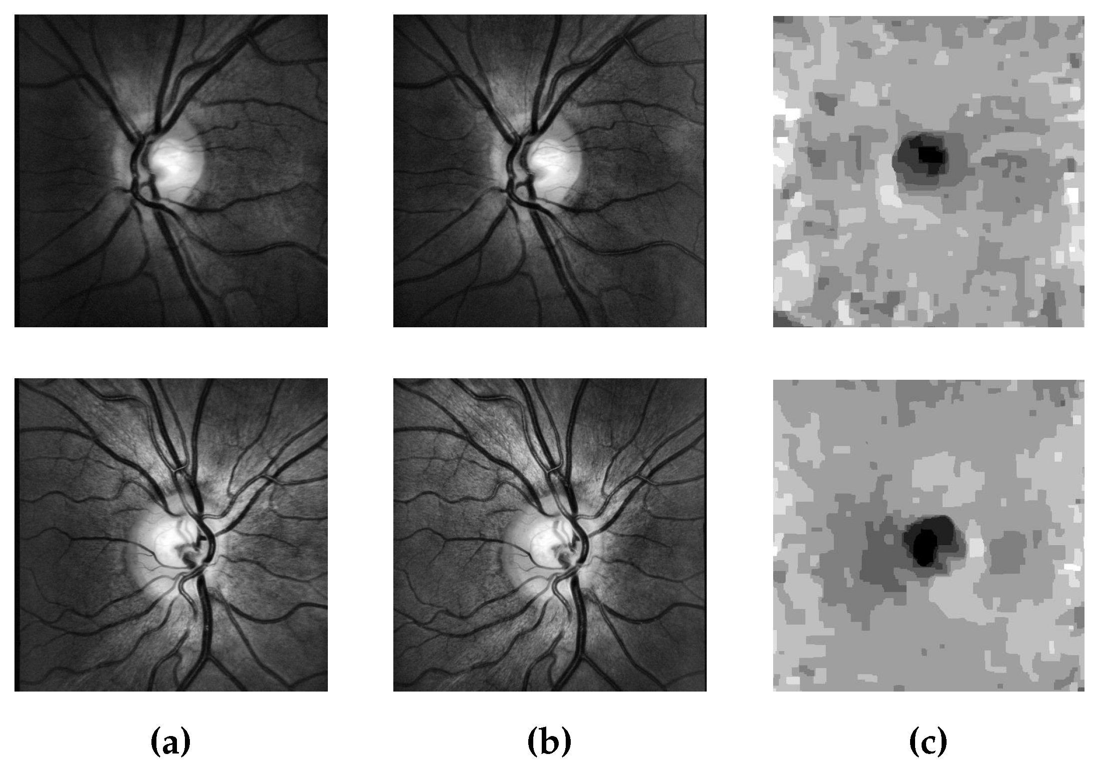
4.2.4. Applications in Biomedical Image Processing

Stereo matching and depth approximation from multi-view datasets have been an attractive area of computer science. The concept is the same as optical flow, since in both, one tries to find the best correspondence between the pixels of the input images. The difference is in the representation of the correspondence between pixels since in optical flow, the view-point is generally constant, while the flow field represents the changes in locations of pixels/objects over time. In contrast, in stereo matching, the scene is mainly still, while the view-point changes, and therefore, the geometric representation of the objects with respect to the camera varies. The formulation of the problem is similar to that of optical flow estimation. The difference is due to the fact that the stereo frames are usually rectified, which means that the displacements are mainly along one of the directions, which makes the process of disparity approximation a 1D problem. With some modifications, which are not the focus of the current work, the formulation can be changed for the problem of stereo matching and disparity approximation. The applications of such a problem can found in various fields, for example retinal image processing. Retinal image processing is a very attractive branch of biomedical image processing [62,63,64]. As an example of such a technique, 3D reconstruction of the Optic Nerve Head (ONH) in the retina can be mentioned. Figure 7 shows two examples of such an application by use of dense SIFT descriptors using the data provided as part of [65]. For each one of these examples, a pair of input images acquired from the left and right views of the ONH (first and second column) is captured, and the approximate depth information is retrieved (third column). The darker the region, the greater the depth. Moreover, the same concept can be used for optical flow estimation and 3D reconstruction of endoscopic and colonoscopic videos. Other applications in 3D reconstruction of microscopic samples using various dense matching techniques have also been explored in the literature [66].

5. Conclusions

The concept of optical flow estimation, as the procedure of finding displacements of intensity patterns in image sequences, has gained much attention in the computer vision community. The general formulation usually involves the minimization of a constrained energy functional for finding the dense flow fields between the images in the sequence. One of the basic assumptions for the formulation is on the brightness level of different regions contained in the images, as it is assumed that the brightness should remain constant regardless of the movement of pixels/objects. This assumption, even though not completely true in general, drives many of the modern day optical flow estimation algorithms. However, many different techniques have been proposed in the recent years, which try to solve the problem in a more general manner. One solution can be sought in formulating the problem by use of more structurally-representative means: local descriptors. Local descriptors have been used in various branches of computer vision, namely object/texture recognition, image retrieval, etc. However, there has been limited investigation on the use of local descriptors for optical flow estimation [34,35].
In the current work, use of several dense descriptors is investigated for optical flow estimation. Given the framework provided by Liu et al. [34], the first aim is to provide a more comprehensive comparison with the state-of-the-art for optical flow estimation, and therefore, several tests are carried out using the Middlebury optical flow datasets [3]. Aiming at extending the framework, the use of seven descriptors, namely the Leung–Malik (LM) filter bank, the Gabor filter bank, the Schmid filter bank, Root Filter Set (RFS) filters, Steerable filters, Histogram of Oriented Gradients (HOG) and Speeded Up Robust Features (SURF), is introduced and investigated here. The presented results show great potential for using dense local descriptors for the problem of optical flow estimation and stereo matching, both in computer vision and also the medical image processing community and can stimulate great interest in devising more rigorous algorithms in the field.

Author Contributions

A. Baghaie designed the study and performed the experiments. The paper is written by A. Baghaie under the supervision of R. M. D’Souza and Z. Yu.

Conflicts of Interest

The authors declare no conflict of interest.

References

  1. Horn, B.K.; Schunck, B.G. Determining optical flow. In Proceedings of the 1981 Technical Symposium East. International Society for Optics and Photonics, Washington, DC, USA, 21 April 1981; pp. 319–331.
  2. Fortun, D.; Bouthemy, P.; Kervrann, C. Optical flow modeling and computation: A survey. Comput. Vis. Image Underst. 2015, 134, 1–21. [Google Scholar] [CrossRef]
  3. Baker, S.; Scharstein, D.; Lewis, J.; Roth, S.; Black, M.J.; Szeliski, R. A database and evaluation methodology for optical flow. Int. J. Comput. Vis. 2011, 92, 1–31. [Google Scholar] [CrossRef]
  4. Vedula, S.; Rander, P.; Collins, R.; Kanade, T. Three-dimensional scene flow. IEEE Trans. Pattern Anal. Mach. Intell. 2005, 27, 475–480. [Google Scholar] [CrossRef]
  5. Brox, T.; Bruhn, A.; Papenberg, N.; Weickert, J. High accuracy optical flow estimation based on a theory for warping. In Proceedings of the 8th European Conference on Computer Vision, Prague, Czech Republic, 11–14 May 2014; pp. 25–36.
  6. Papenberg, N.; Bruhn, A.; Brox, T.; Didas, S.; Weickert, J. Highly accurate optic flow computation with theoretically justified warping. Int. J. Comput. Vis. 2006, 67, 141–158. [Google Scholar] [CrossRef]
  7. Mileva, Y.; Bruhn, A.; Weickert, J. Illumination-robust variational optical flow with photometric invariants. In Pattern Recognition; Springer: Berlin, Germany, 2007; pp. 152–162. [Google Scholar]
  8. Zimmer, H.; Bruhn, A.; Weickert, J.; Valgaerts, L.; Salgado, A.; Rosenhahn, B.; Seidel, H.P. Complementary optic flow. In Energy Minimization Methods in Computer Vision and Pattern Recognition; Springer: Berlin, Germany, 2009; pp. 207–220. [Google Scholar]
  9. Black, M.J.; Anandan, P. The robust estimation of multiple motions: Parametric and piecewise-smooth flow fields. Comput. Vis. Image Underst. 1996, 63, 75–104. [Google Scholar] [CrossRef]
  10. Cohen, I. Nonlinear variational method for optical flow computation. In Proceedings of the 8th Scandinavian Conference on Image Analysis; Tromssa, Norway, 1993; Volume 1, pp. 523–530. [Google Scholar]
  11. Mémin, E.; Pérez, P. Dense estimation and object-based segmentation of the optical flow with robust techniques. IEEE Trans. Image Process. 1998, 7, 703–719. [Google Scholar] [CrossRef] [PubMed]
  12. Lazebnik, S.; Schmid, C.; Ponce, J. A sparse texture representation using affine-invariant regions. In Proceedings of the IEEE Computer Society Conference on Computer Vision and Pattern Recognition, Madison, WI, USA, 16–22 June 2003; Volume 2, pp. 319–324.
  13. Tuzel, O.; Porikli, F.; Meer, P. Region covariance: A fast descriptor for detection and classification. In Computer Vision—ECCV 2006; Springer: Berlin, Germany, 2006; pp. 589–600. [Google Scholar]
  14. Viola, P.; Jones, M. Rapid object detection using a boosted cascade of simple features. In Proceedings of the 2001 IEEE Computer Society Conference on Computer Vision and Pattern Recognition (CVPR 2001), Kauai, HI, USA, 8–14 December 2001; Volume 1, pp. 511–518.
  15. Zhu, Q.; Yeh, M.C.; Cheng, K.T.; Avidan, S. Fast human detection using a cascade of histograms of oriented gradients. In Proceedings of the IEEE Computer Society Conference on Computer Vision and Pattern Recognition, New York, NY, USA, 17–22 June 2006; Volume 2, pp. 1491–1498.
  16. Rublee, E.; Rabaud, V.; Konolige, K.; Bradski, G. ORB: An efficient alternative to SIFT or SURF. In Proceedings of the 2011 IEEE International Conference on Computer Vision (ICCV), Barcelona, Spain, 6–13 November 2011; pp. 2564–2571.
  17. Fei-Fei, L.; Perona, P. A bayesian hierarchical model for learning natural scene categories. In Proceedings of the Computer Society Conference on Computer Vision and Pattern Recognition (CVPR), San Diego, CA, USA, 20–25 June 2005; Volume 2, pp. 524–531.
  18. Csurka, G.; Dance, C.; Fan, L.; Willamowski, J.; Bray, C. Visual categorization with bags of keypoints. In Proceedings of the Workshop on Statistical Learning in Computer Vision (ECCV), Prague, Czech Republic, 15–26 May 2004; Volume 1, pp. 1–2.
  19. Felzenszwalb, P.F.; Girshick, R.B.; McAllester, D.; Ramanan, D. Object detection with discriminatively trained part-based models. IEEE Trans. Pattern Anal. Mach. Intell. 2010, 32, 1627–1645. [Google Scholar] [CrossRef] [PubMed]
  20. Sivic, J.; Zisserman, A. Video Google: A text retrieval approach to object matching in videos. In Proceedings of the Ninth IEEE International Conference on Computer Vision, Nice, France, 13–16 October 2003; pp. 1470–1477.
  21. Mikolajczyk, K.; Schmid, C. A performance evaluation of local descriptors. IEEE Trans. Pattern Anal. Mach. Intell. 2005, 27, 1615–1630. [Google Scholar] [CrossRef] [PubMed]
  22. Johnson, A.E.; Hebert, M. Recognizing objects by matching oriented points. In Proceedings of the IEEE Computer Society Conference on Computer Vision and Pattern Recognition, San Juan, Puerto Rico, 17–19 June 1997; pp. 684–689.
  23. Lowe, D.G. Distinctive image features from scale-invariant keypoints. Int. J. Comput. Vis. 2004, 60, 91–110. [Google Scholar] [CrossRef]
  24. Gabor, D. Theory of communication. Part 1: The analysis of information. J. Inst. Electr. Eng. Part III Radio Commun. Eng. 1946, 93, 429–441. [Google Scholar] [CrossRef]
  25. Vetterli, M.; Kovacevic, J. Wavelets and Subband Coding; Number LCAV-BOOK-1995-001; Prentice-Hall: Upper Saddle River, NJ, USA, 1995. [Google Scholar]
  26. Freeman, W.T.; Adelson, E.H. The design and use of steerable filters. IEEE Trans. Pattern Anal. Mach. Intell. 1991, 13, 891–906. [Google Scholar] [CrossRef]
  27. Baumberg, A. Reliable feature matching across widely separated views. In Proceedings of the IEEE Conference on Computer Vision and Pattern Recognition, Hilton Head, SC, USA, 3–15 June 2000; Volume 1, pp. 774–781.
  28. Schaffalitzky, F.; Zisserman, A. Multi-view matching for unordered image sets, or “How do I organize my holiday snaps?”. In Computer Vision—ECCV 2002; Springer: Berlin, Germany, 2002; pp. 414–431. [Google Scholar]
  29. Wang, H.; Kläser, A.; Schmid, C.; Liu, C.L. Action recognition by dense trajectories. In Proceedings of the IEEE Conference on Computer Vision and Pattern Recognition (CVPR), Colorado Springs, CO, USA, 20–25 June 2011; pp. 3169–3176.
  30. Tola, E.; Lepetit, V.; Fua, P. Daisy: An efficient dense descriptor applied to wide-baseline stereo. IEEE Trans. Pattern Anal. Mach. Intell. 2010, 32, 815–830. [Google Scholar] [CrossRef] [PubMed]
  31. Sangineto, E. Pose and expression independent facial landmark localization using dense-SURF and the Hausdorff distance. IEEE Trans. Pattern Anal. Mach. Intell. 2013, 35, 624–638. [Google Scholar] [CrossRef] [PubMed]
  32. Dalal, N.; Triggs, B. Histograms of oriented gradients for human detection. In Proceedings of the IEEE Computer Society Conference on Computer Vision and Pattern Recognition, San Dieg, CA, USA, 20–25 June 2005; Volume 1, pp. 886–893.
  33. Uijlings, J.; Duta, I.; Sangineto, E.; Sebe, N. Video classification with Densely extracted HOG/HOF/MBH features: An evaluation of the accuracy/computational efficiency trade-off. Int. J. Multimed. Inf. Retr. 2015, 4, 33–44. [Google Scholar] [CrossRef]
  34. Liu, C.; Yuen, J.; Torralba, A. Sift flow: Dense correspondence across scenes and its applications. IEEE Trans. Pattern Anal. Mach. Intell. 2011, 33, 978–994. [Google Scholar] [CrossRef] [PubMed]
  35. Brox, T.; Malik, J. Large displacement optical flow: Descriptor matching in variational motion estimation. IEEE Trans. Pattern Anal. Mach. Intell. 2011, 33, 500–513. [Google Scholar] [CrossRef] [PubMed]
  36. Baghaie, A.; D’Souza, R.M.; Yu, Z. Dense Correspondence and Optical Flow Estimation Using Gabor, Schmid and Steerable Descriptors. In Advances in Visual Computing; Springer: Berlin, Germany, 2015; pp. 406–415. [Google Scholar]
  37. Leung, T.; Malik, J. Representing and recognizing the visual appearance of materials using three-dimensional textons. Int. J. Comput. Vis. 2001, 43, 29–44. [Google Scholar] [CrossRef]
  38. Schmid, C. Constructing models for content-based image retrieval. In Proceedings of the 2001 IEEE Computer Society Conference on Computer Vision and Pattern Recognition (CVPR), Kauai, HI, USA, 8–14 December 2001; Volume 2, pp. 39–45.
  39. Bay, H.; Ess, A.; Tuytelaars, T.; Van Gool, L. Speeded-up robust features (SURF). Comput. Vis. Image Underst. 2008, 110, 346–359. [Google Scholar] [CrossRef]
  40. Bernal, J.; Vilarino, F.; Sánchez, J. Feature Detectors and Feature Descriptors: Where We Are Now; Universitat Autonoma de Barcelona: Barcelona, Spain, 2010. [Google Scholar]
  41. Movellan, J.R. Tutorial on Gabor filters. Open Source Document. 2002. Available online: http://mplab.ucsd.edu/tutorials/gabor.pdf (accessed on 25 February 2017).
  42. Ilonen, J.; Kämäräinen, J.K.; Kälviäinen, H. Efficient Computation of Gabor Features; Lappeenranta University of Technology: Lappeenranta, Finland, 2005. [Google Scholar]
  43. Varma, M.; Zisserman, A. A statistical approach to texture classification from single images. Int. J. Comput. Vis. 2005, 62, 61–81. [Google Scholar] [CrossRef]
  44. Jacob, M.; Unser, M. Design of steerable filters for feature detection using canny-like criteria. IEEE Trans. Pattern Anal. Mach. Intell. 2004, 26, 1007–1019. [Google Scholar] [CrossRef] [PubMed]
  45. Aguet, F.; Jacob, M.; Unser, M. Three-dimensional feature detection using optimal steerable filters. In Proceedings of the IEEE International Conference on Image Processing (ICIP), Genova, Italy, 11–14 September 2005; Volume 2, pp. 1158–1161.
  46. Brown, M.; Lowe, D.G. Invariant Features from Interest Point Groups; BMVC 2002: 13th British Machine Vision Conference; University of Bath: Bath, England, 2002. [Google Scholar]
  47. Lindeberg, T. Scale-space theory: A basic tool for analyzing structures at different scales. J. Appl. Stat. 1994, 21, 225–270. [Google Scholar] [CrossRef]
  48. Mikolajczyk, K.; Schmid, C. An affine invariant interest point detector. In Computer Vision—ECCV 2002; Springer: Berlin, Germany, 2002; pp. 128–142. [Google Scholar]
  49. Barber, D. Bayesian Reasoning and Machine Learning; Cambridge University Press: Cambridge, UK, 2012. [Google Scholar]
  50. Pearl, J. Probabilistic Reasoning in Intelligent Systems: Networks Of Plausible Inference; Morgan Kaufmann: Burlington, MA, USA, 2014. [Google Scholar]
  51. Szeliski, R.; Zabih, R.; Scharstein, D.; Veksler, O.; Kolmogorov, V.; Agarwala, A.; Tappen, M.; Rother, C. A comparative study of energy minimization methods for markov random fields with smoothness-based priors. IEEE Trans. Pattern Anal. Mach. Intell. 2008, 30, 1068–1080. [Google Scholar] [CrossRef] [PubMed]
  52. Murphy, K.P.; Weiss, Y.; Jordan, M.I. Loopy belief propagation for approximate inference: An empirical study. In Proceedings of the Fifteenth Conference on Uncertainty in Artificial Intelligence, Stockholm, Sweden, 30 July–1 August 1999; Morgan Kaufmann Publishers Inc.: Burlington, MA, USA, 1999; pp. 467–475. [Google Scholar]
  53. Kschischang, F.R.; Frey, B.J.; Loeliger, H.A. Factor graphs and the sum-product algorithm. IEEE Trans. Inf. Theory 2001, 47, 498–519. [Google Scholar] [CrossRef]
  54. Geiger, A.; Lenz, P.; Urtasun, R. Are we ready for Autonomous Driving? The KITTI Vision Benchmark Suite. In Proceedings of the 2012 IEEE Conference on Computer Vision and Pattern Recognition (CVPR), Providence, RI, USA, 16–21 June 2012.
  55. yves Bouguet, J. Pyramidal Implementation of the Lucas Kanade Feature Tracker; Intel: Longmont, CO, USA, 2000. [Google Scholar]
  56. Le Besnerais, G.; Champagnat, F. Dense optical flow by iterative local window registration. In Proceedings of the IEEE International Conference on Image Processing (ICIP), Genova, Italy, 11–14 September 2005; Volume 1, pp. 137–140.
  57. Corpetti, T.; Mémin, E. Stochastic uncertainty models for the luminance consistency assumption. IEEE Trans. Image Process. 2012, 21, 481–493. [Google Scholar] [CrossRef] [PubMed] [Green Version]
  58. Alba, A.; Arce-Santana, E.; Rivera, M. Optical flow estimation with prior models obtained from phase correlation. In Advances in Visual Computing; Springer: Berlin, Germany, 2010; pp. 417–426. [Google Scholar]
  59. Solari, F.; Chessa, M.; Medathati, N.K.; Kornprobst, P. What can we expect from a V1-MT feedforward architecture for optical flow estimation? Signal Process. Image Commun. 2015, 39, 342–354. [Google Scholar] [CrossRef] [Green Version]
  60. Van De Sande, K.E.; Gevers, T.; Snoek, C.G. Evaluating color descriptors for object and scene recognition. IEEE Trans. Pattern Anal. Mach. Intell. 2010, 32, 1582–1596. [Google Scholar] [CrossRef] [PubMed]
  61. Trulls, E.; Kokkinos, I.; Sanfeliu, A.; Moreno-Noguer, F. Dense segmentation-aware descriptors. In Proceedings of the IEEE Conference on Computer Vision and Pattern Recognition, Portland, OR, USA, 23–28 June 2013; pp. 2890–2897.
  62. Baghaie, A.; Yu, Z.; D’Souza, R.M. State-of-the-art in retinal optical coherence tomography image analysis. Quant. Imaging Med. Surg. 2015, 5, 603. [Google Scholar] [PubMed]
  63. Baghaie, A.; D’souza, R.M.; Yu, Z. Application of Independent Component Analysis Techniques in Speckle Noise Reduction of Single-Shot Retinal OCT Images. arXiv 2015. [Google Scholar]
  64. Baghaie, A.; D’souza, R.M.; Yu, Z. Sparse and low rank decomposition based batch image alignment for speckle reduction of retinal OCT images. In Proceedings of the 2015 IEEE 12th International Symposium on Biomedical Imaging (ISBI), New York, NY, USA, 16–19 April 2015; pp. 226–230.
  65. Pena-Betancor, C.; Gonzalez-Hernandez, M.; Fumero-Batista, F.; Sigut, J.; Medina-Mesa, E.; Alayon, S.; de la Rosa, M.G. Estimation of the Relative Amount of Hemoglobin in the Cup and Neuroretinal Rim Using Stereoscopic Color Fundus ImagesNeuroretinal Rim Hemoglobin. Investig. Ophthalmol. Vis. Sci. 2015, 56, 1562–1568. [Google Scholar] [CrossRef] [PubMed]
  66. Baghaie, A. Study of Computational Image Matching Techniques: Improving Our View of Biomedical Image Data. Ph.D. Thesis, University of Wisconsin-Milwaukee (UWM), Milwaukee, WI, USA, 2016. [Google Scholar]
Figure 1. Samples of the filter banks used for creating the dense descriptors: (a) Leung–Malik (LM), (b) the real part of the Gabor (G), (c) Schmid (S), (d) Root Filter Set (RFS) and (e) Steerable (St) filters.
Jimaging 03 00012 g001
Figure 2. Sample HOG with eight directions for Badafshan.
Jimaging 03 00012 g002
Figure 3. Factor graph representation of the energy minimization functional with de-coupled horizontal and vertical components.
Jimaging 03 00012 g003
Figure 4. (a) The set of input image pairs (gray-valued images), as well as the ground truth (colored images) of the optical flow used for assessing the performance of the eight dense descriptors for optical flow estimation; (b) code for the visualization of the flow fields.
Jimaging 03 00012 g004
Figure 5. Sample results of the optical flow estimation for Grove2 (first row), Grove3 (second row), RubberWhale (third row) and Venus (fourth row) using the eight dense descriptors, d-Gabor (a), d-Schmidt (b), d-LM (c), d-RFS (d), d-Steerable (e), d-HOG (f), d-SURF (g) and d-SIFT (h).
Jimaging 03 00012 g005
Figure 6. Sample results of the optical flow estimation for two of the test image sets from Middlebury Mequon and Teddy, as well as the flow error, using SLK [57] (first column), PGAM + LK [58] (second column), FFV1MT [59] (third column), d-SURF (fourth column) and d-SIFT (fifth column).
Jimaging 03 00012 g006
Figure 7. Retina Optic Nerve Head (ONH) depth approximation by use of stereo image pairs: (a) left view; (b) right view; (c) approximated depth map. The darker the region, the greater the depth.
Jimaging 03 00012 g007
Table 1. Number of dimensions (Dim.) of the dense descriptors.
Methodd-Gabord-Schmidd-LMd-RFSd-Steerabled-HOGd-SURFd-SIFT
# of Dim.801348384020064128
Table 2. Average Angular Error (AAE) comparison for training images of the Middlebury dataset.
MethodDimetrodonGrove2Grove3HydrangeaRubberWhaleUrban2Urban3VenusAvg. Rank
d-Gabor16.438.1113.2710.9813.4728.0918.649.304.50
d-Schmid18.8712.5517.4915.0517.5016.0818.1514.777.00
d-LM18.4212.7617.0512.3615.8219.3618.4811.886.62
d-RFS19.0610.2015.7011.8313.7514.5417.168.685.37
d-Steerable21.188.7313.8213.7713.6112.6716.836.804.75
d-HOG16.248.6012.999.8611.0928.3016.006.453.12
d-SURF17.998.9712.7210.5110.7314.2713.816.782.87
d-SIFT17.248.2912.229.7710.4714.6711.024.791.75
Table 3. Average Endpoint Error (AEE) comparison for training images of the Middlebury dataset.
MethodDimetrodonGrove2Grove3HydrangeaRubberWhaleUrban2Urban3VenusAvg. Rank
d-Gabor0.5040.6561.3430.5980.4246.4323.0050.6093.25
d-Schmid0.6500.9071.7210.7370.5192.3893.4540.9526.87
d-LM0.6260.9371.6260.6130.4794.2233.1730.9166.00
d-RFS0.6510.7851.6080.5500.4352.2183.3410.6385.12
d-Steerable2.6810.7511.4563.4620.4381.8823.3990.5815.25
d-HOG0.5040.6961.3600.4020.3696.4483.4590.4783.75
d-SURF0.6470.7401.3780.4470.3621.9893.9360.5653.87
d-SIFT0.5630.6871.3050.3930.3562.3213.0150.4011.87
Table 4. Interpolation Error (IE) comparison for training images of the Middlebury dataset.
MethodDimetrodonGrove2Grove3HydrangeaRubberWhaleUrban2Urban3VenusAvg. Rank
d-Gabor3.599.8015.117.263.5414.978.506.347.00
d-Schmid3.4910.0015.357.073.715.636.326.736.87
d-LM3.4610.2314.996.583.459.465.756.525.87
d-RFS3.399.1912.726.103.164.555.786.243.25
d-Steerable11.139.4113.3210.503.124.766.036.335.37
d-HOG3.289.0612.516.143.1914.105.275.863.00
d-SURF3.158.7111.505.523.124.225.495.751.25
d-SIFT3.319.3013.156.403.344.705.276.003.75
Table 5. Average (standard deviation) of angular error comparisons for the Middlebury test dataset.
MethodArmyMequonScheffleraWoodenGroveUrbanYosemiteTeddyAverage Ranking
Pyramid LK [55]13.9(17.0)24.1(31.7)20.9(32.9)22.2(29.4)18.7(31.7)21.2(29.9)6.41(9.01)25.6(39.9)118.0(119.4)
FOLKI [56]10.5(16.2)20.9(32.5)17.6(29.4)15.4(29.1)6.16(9.58)12.2(25.7)4.67(7.71)18.2(36.5)115.2(116.0)
SLK [57]11.6(17.2)15.3(21.3)17.8(27.9)25.4(31.4)5.25(6.6)10.3(22.8)2.89(3.90)14.9(33.3)110.1(108.9)
PGAM+ LK [58]11.8(14.9)14.8(25.5)13.2(21.9)16.2(26.0)5.40(9.61)12.3(24.3)7.42(6.19)13.2(34.3)113.5(108.7)
FFV1MT [59]12.0(13.9)10.7(20.9)15.6(21.8)16.6(31.0)6.51(9.97)16.2(23.8)3.41(2.99)12.3(37.6)110.8(106.1)
d-SURF13.2(11.7)8.96(11.1)11.4(17.8)11.3(16.9)10.6(11.3)19.7(29.2)17.0(15.8)8.34(29.3)108.8(96.9)
d-SIFT13.3(12.1)8.66(10.9)10.7(15.8)10.9(15.9)9.70(8.33)15.4(22.6)14.5(11.3)7.89(30.0)107.9(92.4)
Table 6. Average (standard deviation) of endpoint error comparisons for the Middlebury test dataset.
MethodArmyMequonScheffleraWoodenGroveUrbanYosemiteTeddyAverage Ranking
Pyramid LK [55]0.39(0.68)1.67(1.94)1.50(2.43)1.57(2.36)2.94(4.19)3.33(7.35)0.30(0.57)3.20(4.63)118.1(118.7)
FOLKI [56]0.29(0.55)1.52(2.45)1.23(2.12)0.99(1.75)1.53(2.10)2.14(5.86)0.26(0.52)2.67(5.03)114.8(117.0)
SLK [57]0.30(0.47)1.09(1.13)1.25(2.12)1.56(1.72)1.54(1.86)2.02(5.75)0.17(0.32)2.43(3.61)109.9(107.7)
PGAM + LK [58]0.37(0.66)1.08(1.64)0.94(1.46)1.40(2.59)1.37(1.75)2.10(6.62)0.36(0.40)1.89(2.95)113.7(106.5)
FFV1MT [59]0.33(0.41)0.79(1.11)1.33(1.62)1.38(2.02)1.76(2.00)2.33(4.48)0.16(0.18)1.81(3.19)109.9(102.1)
d-SURF0.37(0.36)0.84(0.79)1.70(1.75)1.04(1.31)2.04(2.21)2.61(5.91)0.91(1.16)1.28(2.94)112.3(107.3)
d-SIFT0.37(0.34)0.82(0.73)1.61(1.52)1.01(1.22)1.98(1.98)2.35(5.66)0.70(0.63)1.21(2.77)110.8(101.8)

