Review

Imaging with Polarized Neutrons

1
Institute of Applied Materials, Helmholtz-Zentrum-Berlin, 14109 Berlin, Germany
2
Technische Universität Berlin, Institut für Werkstoffwissenschaften und –technologien, 10623 Berlin, Germany
3
Laboratory for Neutron Scattering and Imaging (LNS), Paul-Scherrer-Institute, 5232 Villigen, Switzerland
4
Niels Bohr Institute, University of Copenhagen, 2100 Copenhagen, Denmark
*
Author to whom correspondence should be addressed.
J. Imaging 2018, 4(1), 23; https://doi.org/10.3390/jimaging4010023
Submission received: 1 November 2017 / Revised: 29 December 2017 / Accepted: 11 January 2018 / Published: 16 January 2018
(This article belongs to the Special Issue Neutron Imaging)

Abstract

:
Owing to their zero charge, neutrons are able to pass through thick layers of matter (typically several centimeters) while being sensitive to magnetic fields due to their intrinsic magnetic moment. Therefore, in addition to the conventional attenuation contrast image, the magnetic field inside and around a sample can be visualized by detecting changes of polarization in a transmitted beam. The method is based on the spatially resolved measurement of the cumulative precession angles of a collimated, polarized, monochromatic neutron beam that traverses a magnetic field or sample.

1. Introduction

Conventional methods for imaging magnetic fields are limited to the surface and the surrounding of a sample [1]. The observation of spatial distribution of magnetic fields inside a bulk sample was not possible heretofore. In order to solve this problem, a new imaging technique utilizing polarized neutrons was proposed [2,3,4]. The method allows one to reveal the three-dimensional distribution of magnetic fields in solid materials.
Neutrons are subatomic particles with no electric charge, which allows them to penetrate thick layers of matter. They possess a magnetic moment making them sensitive to magnetic fields [5]. Utilizing the associated magnetic interaction for neutron imaging it is possible to visualize magnetic fields not only in free space but also in the bulk of samples.
In an applied magnetic field of strength B, the spin of the neutron, which is always aligned anti-parallel to its magnetic moment, will undergo Larmor precession around the field with a precession frequency ω L = γ B , where γ is the gyromagnetic ratio of the neutron (−1.832 × 10⁸ rad s−1 T−1) and B is the scalar magnitude of the magnetic field. If the field has a significant component perpendicular to the magnetic moment of the neutron, precession will cause the neutrons to oscillate between the two possible spin-states (spin up and spin down states).
For a neutron traversing a magnetic field, the rate of precession is related to the strength of the field, and the total angle of precession φ is proportional to the field strength B , the wavelength of the neutrons λ and the length of the path s through the field: φ = γ λ m h path   B d s , where m is the neutron rest mass (1.675 × 10⁻²⁷ kg) and h is Planck’s constant (6.626 × 10⁻³⁴ J s−1) [6]. Thus, for a monochromatic beam, variations in the total precession angle for a given path through a magnetic field are indicative of the distribution of the field along that path [7,8]. These variations can be measured using a polarized beam, i.e., one in which all neutrons of one of the two possible spin-states have been removed from the beam. The polarization vector, P, may be considered as the average spin orientation over the whole beam and it is possible to consider precession of the polarization rather than of each individual neutron spin.

2. Experimental Techniques

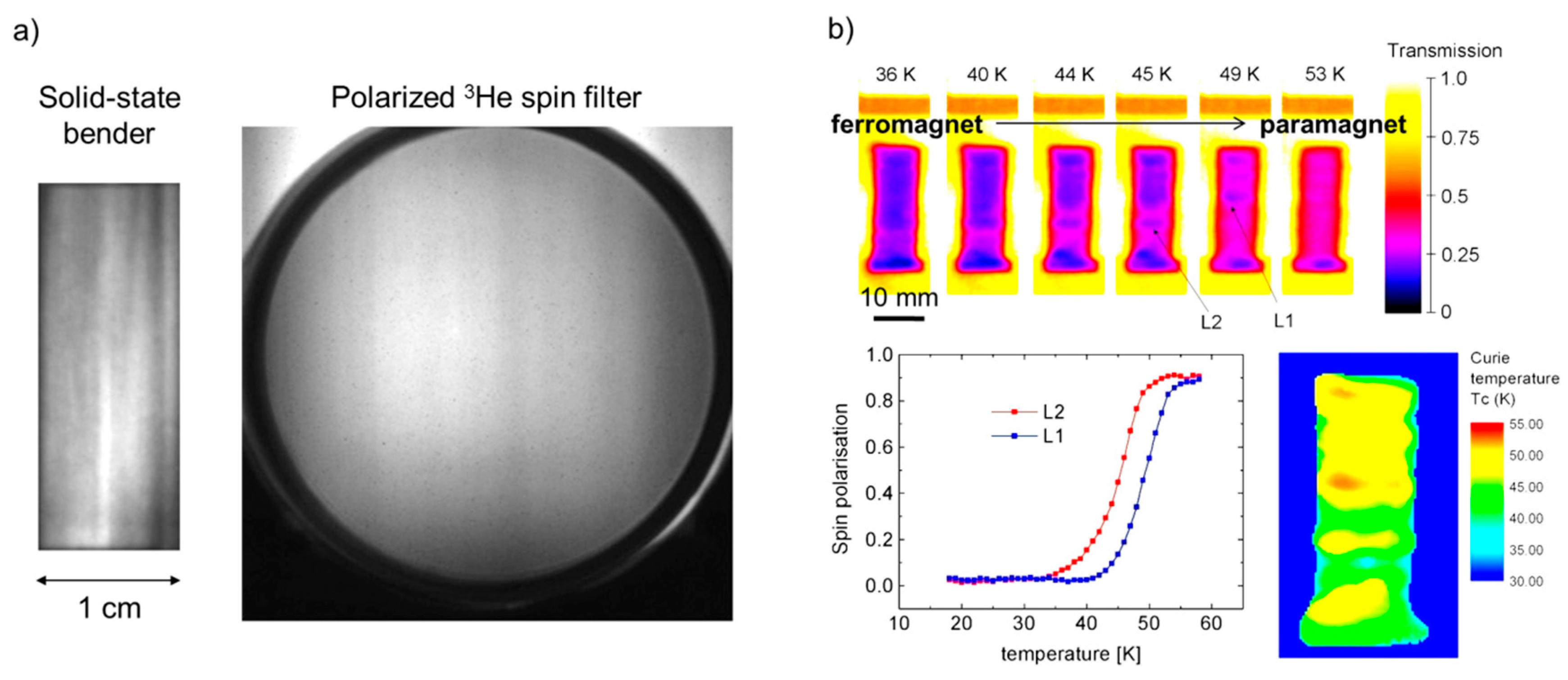
2.1. Solid-State Benders

Magnetic imaging experiments with polarized neutrons have recently been undertaken at various imaging facilities. The first experiments were performed with a polarizer-analyzer arrangement based on solid state benders [2]. These benders consist of thin plates, usually Si wafers, which are covered on one side by a super mirror layer reflecting neutrons according to classical optics principles [9].
Applying strong magnetic fields of several tenths mT perpendicular to the propagation direction of the neutrons, different refractive indices for spin-up and -down neutrons occur and cause a different deflection of the two spin states, thus giving rise to two sub-beams possessing different directions. By using a collimator or by covering the non-reflecting surface of the substrates by a strongly absorbing layer (e.g., Gd) one spin component can be selected. In this way, a setup for magnetic imaging is obtained in which a solid-state bender is used to polarize a neutron beam, which is then directed through magnetic samples in which precession sets in before the beam is analyzed with a second bender [3], Figure 1a. The key to image formation is that the analyzer only transmits the polarization component that is parallel to its own polarization axis. As a result, the intensity measured behind the analyzer I is the initial beam intensity I0 decreased by conventional attenuation with attenuation coefficient Σ (the magnitude of which can be found from a standard radiograph) and modulated by some sinusoidal function that is directly related to the angle ϕ by which the polarization has precessed: I = I 0 exp ( path   Σ ( s ) d s ) 1 2 ( 1 + cos ( φ ) ) . Maximum (minimum) intensity will be measured whenever beam polarization and the analyzer are aligned perfectly in parallel (anti-parallel).
This has been demonstrated with a variety of magnetic systems. Figure 1b reveals the familiar pattern of field lines around a simple dipole magnet, while Figure 1c shows the field around a magnet that is levitating over a cooled YBCO superconductor due to the Meissner effect. The rainbow color scale (from blue = minimum to red = maximum) used in the images is related to the intensity variations induced by the sample and by the applied magnetic field. The decay of the magnetic field with distance creates an annular structure of minima (blue) and maxima (red) representing the 2π periodical rotation of the neutron spin. The imaging method can also be extended into three dimensions using a standard tomographic technique in some instances as indicated in Figure 1d, which shows the distribution of a magnetic field trapped inside a lead cylinder that becomes superconductive when cooled below the critical temperature of Tc = 7.2 K [2,3].
With the experimental setup presented one can investigate not only static states at constant magnetic field but also the dynamics of fields produced by AC currents with high frequencies. Interesting examples are the visualization of the skin effect in bulk conductors [10] or the magnetic field produced by a solenoid driven with a high-frequency (3 kHz) AC current [11] as presented in Figure 2. In order to obtain images in short time intervals a stroboscopic method was applied where the detector was triggered by a signal from the power generator to take images at the same current amplitudes many times. The obtained images for a given current amplitude were summed up to obtain an image with reasonable signal-to-noise ratio.
The benders have several properties that are not ideal for imaging experiments aiming at high-spatial resolution: (i) for polarizers working in the reflection mode the polarized neutron beam is deflected. This implies that sample and detector must be shifted transversally in order to be aligned with the beam; (ii) the available field of view is relatively small (1 to 4 cm), which is a problem for investigations of large samples and their surroundings; (iii) the bender collimates the beam along one direction, resulting in a significantly lower resolution along the other direction; (iv) the beam polarization is not uniform across the beam (it can fluctuate by up to 5%); (v) the beam attenuation caused by the wafers causes strong striping inhomogeneities in the beam intensity profile (Figure 3a); and (vi) the comparably strong magnets (0.1 T) needed to magnetize the benders require a sample-bender separation of ~50 cm to ensure that the interaction between the magnetic field of the bender and that of the sample is negligible. This separation distance is a reason for geometrical blurring caused by the finite divergence of the beam.

2.2. Polarized 3He Spin Filters

The nuclear orbital moment of 3He atoms can be polarized by optical pumping using the SEOP (spin-exchange) method. For the interaction of neutrons with the polarized 3He gas in constant magnetic field, different absorption coefficients for parallel and anti-parallel neutron spin orientations with respect to the 3He atoms can be obtained. In this way, only one spin component of the neutrons will be transmitted through the cell. The cells are made of glass and are filled with polarized 3He gas under a certain pressure. They are placed in several 10-cm long boxes in which a constant magnetic field is held. The spin filters do not alter the angular distribution of the beam and in this way do not affect spatial resolution (aside from the geometrical spread as the beam passes them) and produce homogeneous attenuation and polarization over the whole beam. A further advantage of 3He cells is that they will accept and polarize neutrons over a large solid angle so that even a poorly collimated beam can be effectively polarized [12].
By emitting radiofrequency pulses with the Larmor frequency of the 3He nuclei, transitions between the 3He spin-states can be induced, allowing the polarizer and the analyzer to be realigned parallel or anti-parallel. Flipping the polarization of the spin filters is equivalent to flipping the polarization of the incident beam with an efficiency of 100% regardless of the neutron wavelength (although in practice there is a loss in polarization of ~10−5 for each flip).
A crucial advantage of the use of filters over benders is that the magnetic field in the box is weak and well confined, allowing samples to be placed close to the front of (and in some cases even inside) the box. By attaching the scintillator directly to the rear surface of the analyzer cell, it is possible to reduce the sample–detector separation to ~15–20 cm, which brings down geometrical blur to ~200 µm [12].
The large and homogenous polarized neutron beam produced by the arrangement of 3He spin filters has been used successfully for mapping phase transitions between ferromagnetic and paramagnetic states in a PdNi crystal with 3.24% Ni as shown in Figure 3b [13]. The ferromagnetic material is characterized by the presence of arbitrarily oriented magnetic domains that depolarize the neutron beam and provide low neutron transmission. After increasing the temperature in some areas, the material becomes paramagnetic, which is characterized by the loss of the domain structure and the neutron beam is no longer depolarized and a rise in transmission is observed. The temperature of the sudden change of neutron transmission is taken as the critical temperature of the phase transition (the Curie temperature). The obtained Curie temperature map provides information about the inhomogeneity of Ni concentration that influences the critical temperature of the PdNi crystal.
The drawbacks of 3He spin filters are the lower polarization ratio in comparison to solid state benders and the decay of the cell polarization with the time. In order to overcome the last drawback cells were developed and used recently for imaging in on-line pumping allowed to maintain polarisation [14]. A detailed comparison between solid-state benders and 3He cells is presented elsewhere [12].

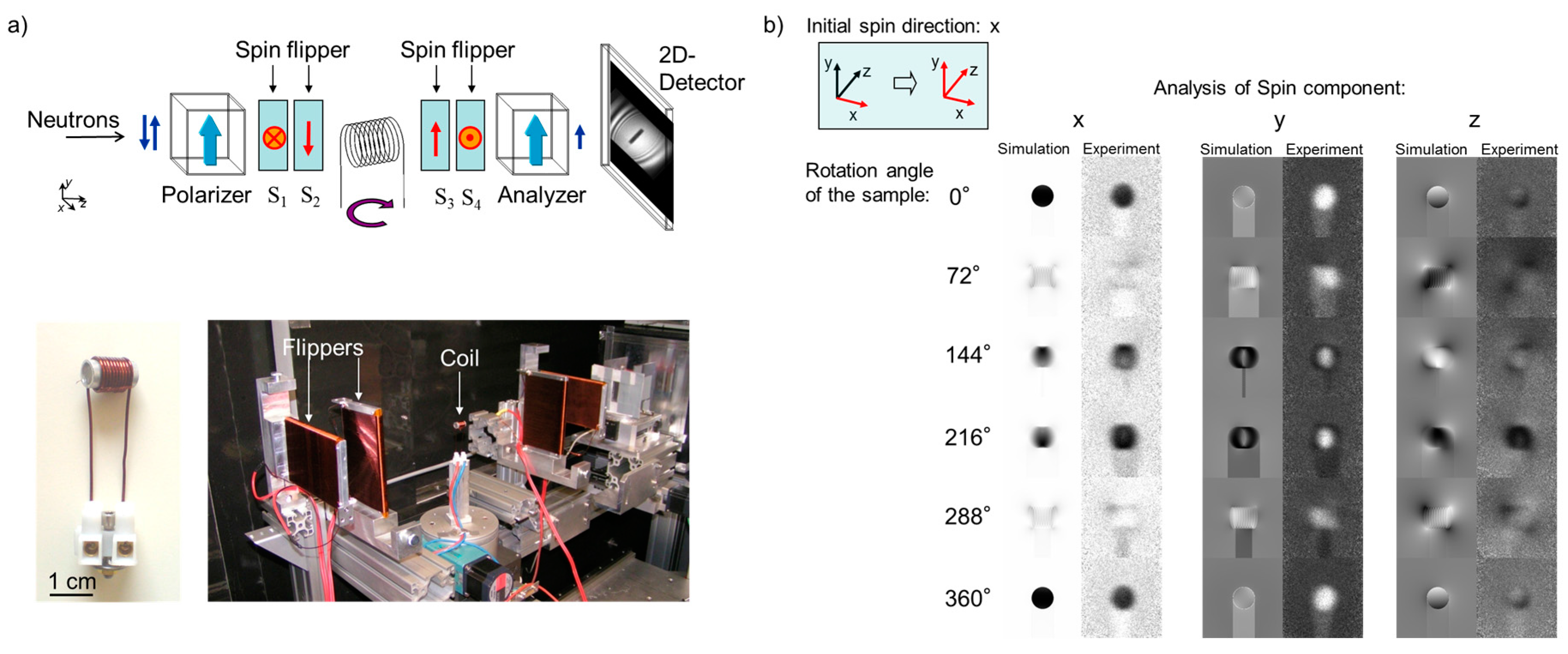
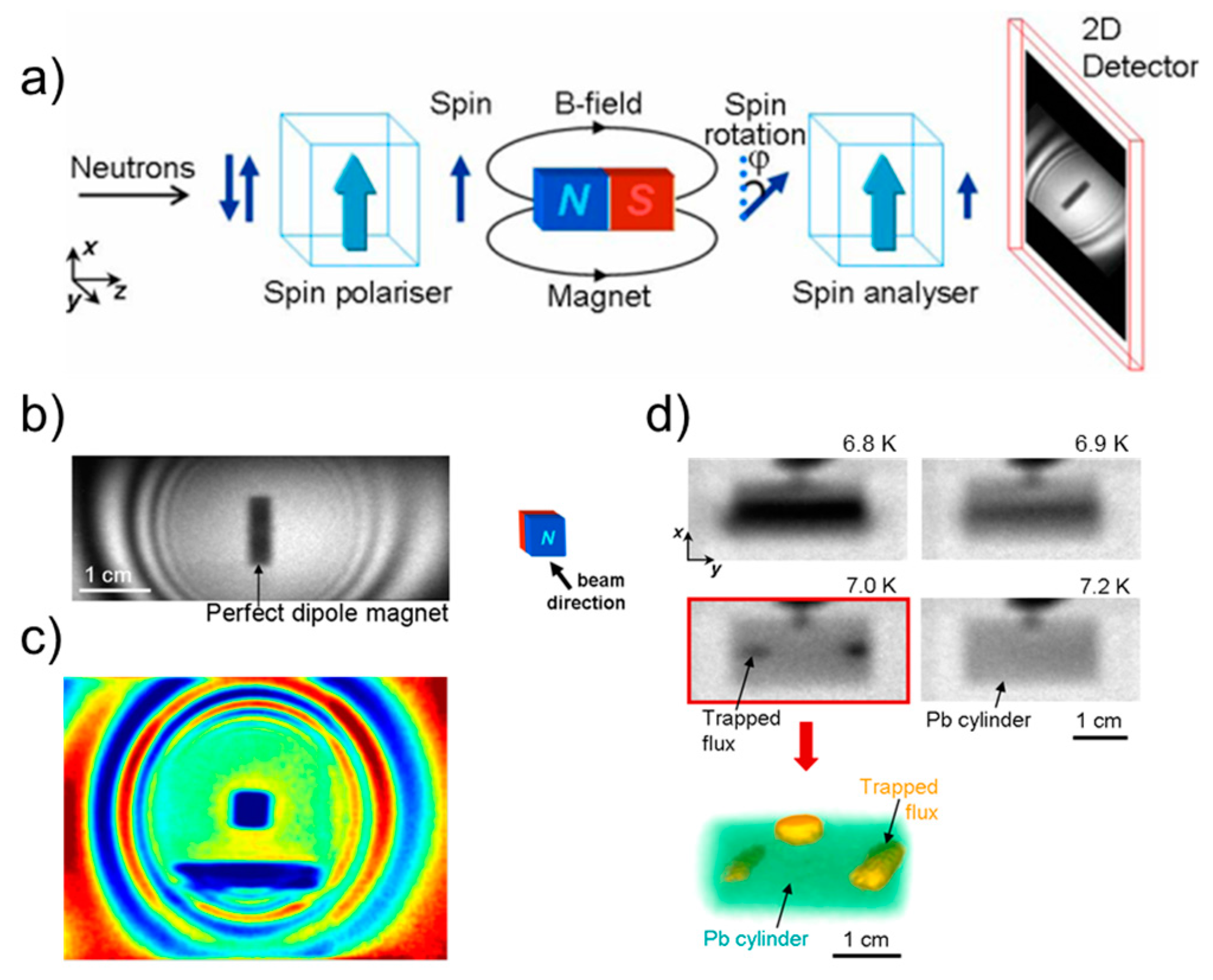
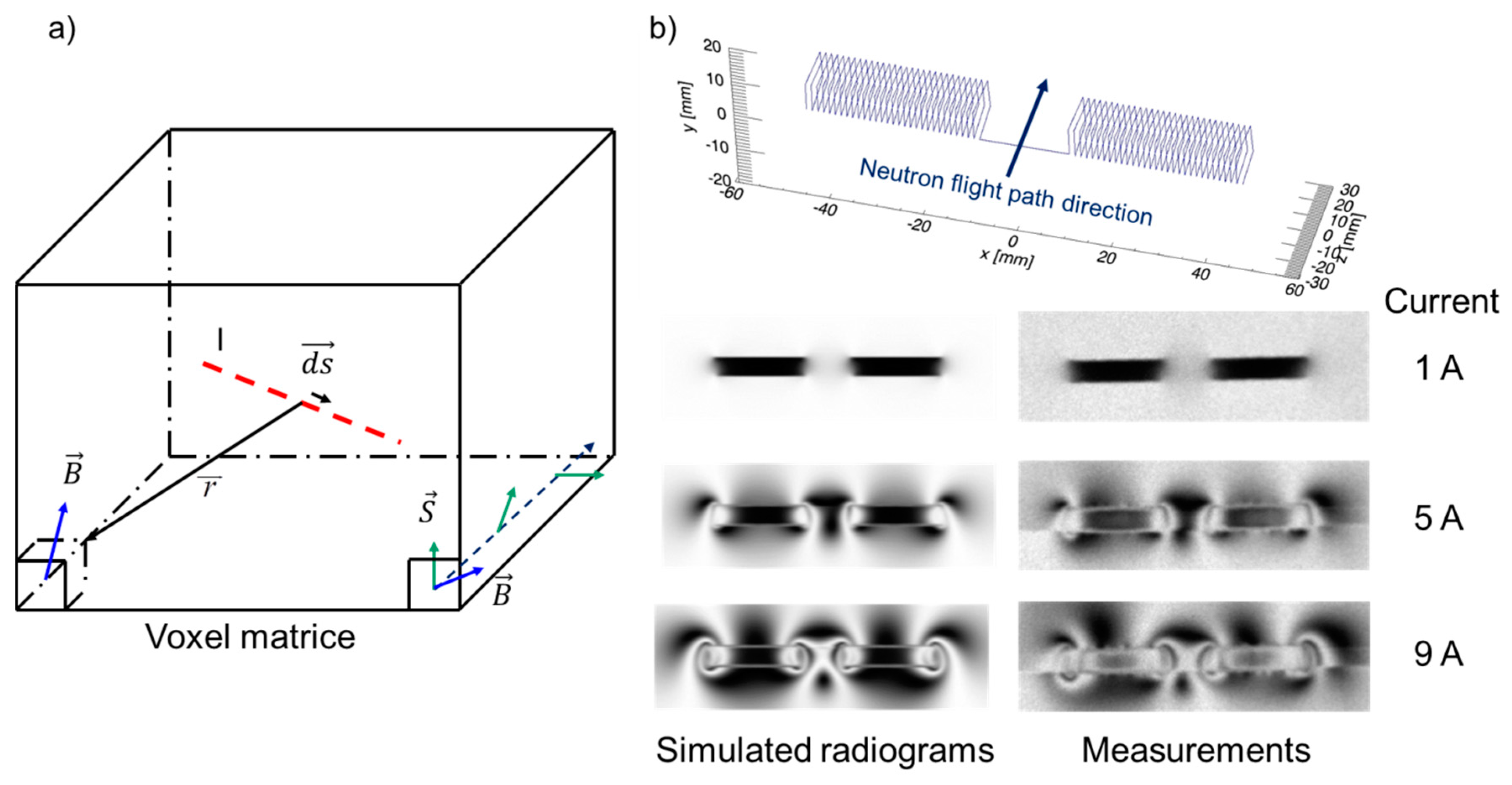
3. Simulation and Quantification of Magnetic Fields

In relatively simple cases, in which the magnetic field distribution of a sample is either well known (e.g., a permanent dipole magnet) or calculable (e.g., via the laws of electromagnetism) it is possible to compare the experimentally measured precession angle to calculated predictions. In the case of a well-known electrical current distribution flowing through a wire, the electromagnetically induced field can be calculated from the Biot–Savart law:
B ( s ) = µ 0 4 π · I · d s × r r 3
where B is the field vector, μ0 the permeability of free space (4π × 10−7 Hm−1), I is the current flowing in the wire, d s is an infinitesimal vector element of the wire pointing in the direction of the current, and r and r are the unit vector and the distance, respectively, from the wire to the point where the field is to be calculated. Starting from Equation (1), the overall local spin rotation at a given point is then given by:
φ =   γ · t · B ,   where   t ~ λ
Once the field distribution of the system is known, it can be used to compute a 3D magnetic field matrix, with each element representing the magnetic field vector in a unit volume (a voxel). Neutrons with a defined polarization vector enter the first voxel and precess for a given time (depending on neutron velocity), leading to a new polarization vector, which is then passed to the next voxel along the trajectory of the neutron, and so on, Figure 4a. Once the neutrons have passed through the matrix the total angle of precession can be used together with (1) to find the intensity measured in the calculated image. Figure 4b shows the experimentally measured and calculated field around a pair of small solenoids with rectangular cross section, separated by 20 mm and supported by an aluminum rod as the direct current passing through them was varied. The coils had roughly the same length of 24.4 mm, a height of 7.5 mm, a depth of 21.5 mm, and 30 windings [3].
In general, the calculated and experimental results agree very well, though some deviations can be seen. These discrepancies occur because the calculations represent an idealized system where the coils are identical, perfectly aligned, self-contained and isolated from external influences. In reality, the coils used in the experiments suffer from irregularities due to their manufacture and differences in the measured intensity (between experiment and calculation) occur.
For the quantification of magnetic vector fields in 3D, a neutron polarimetric setup is used. The spin of the polarized neutron beam is rotated by spin flippers (rotators) in order to send one of the three orthogonal components x, y or z through the sample and in the same way the resulting spin orientation after precession in the magnetic field of the sample is analyzed by a second spin flipper (rotator) for each of the x, y or z directions. From these 9 measurements (one initial component x, y or z is analyzed in each of the three components (x, y, z) of the spin precession angle) for each pixel of the detector, the polarization matrix P can be reconstructed correspondingly. Applying a tomographic approach, it is possible to reconstruct the modulus and the x, y, z components of the magnetic field vector for each point of the sample’s volume and the space around it. Several approaches were developed and tested on simple samples with well-defined magnetic field distributions, e.g., a small solenoid producing a static magnetic field under DC current. The first results are shown in Figure 5, where a small solenoid was investigated by neutron tomography using the polarimetric arrangement at a steady state neutron source (research reactor). An iterative procedure based on simulations (Biot-Savart law) shows a good agreement with the experimental data and allows for a 3D visualization of the field produced by the solenoid [7]. A different approach using a pulsed neutron beam combined with a time-of-flight method was proposed recently and first experiments show promising reconstructions of the magnetic vector field produced by a current driven solenoid obtained by the Filtered-Back-Projection tomographic reconstruction algorithm [15].

4. Conclusions

Spin-polarized neutron imaging is a non-destructive and non-invasive method that has a number of advantages compared to 2D imaging techniques using garnet films or scanning techniques (for magnetic fields outside the sample). The method is applicable to very different environmental set-ups (e.g., for low or high temperature investigations) and samples can be investigated from almost any viewing angle. In this way, 3D information about the field distribution is revealed even if no mathematical tomographic reconstruction is applied. Measurements are fast because about one million pixels are acquired in only one image within a few seconds or minutes. No other method can compete with these advantages even for field measurements in free space. Time and spatially resolved measurements become possible.
The presence and controlled application of magnetic fields is essential in many fields of science and technology as well as in fundamental physics. For example, investigations of flux distribution and flux pinning in large superconducting samples, the skin effect in conductors or magnetic domain distributions in bulk ferromagnets can be visualized and studied in detail.

Conflicts of Interest

The authors declare no conflict of interest.

References

  1. De Graef, M.; Zhu, Y. Preface. In Experimental Methods in the Physical Sciences; Marc De, G., Yimei, Z., Eds.; Academic Press: New York, NY, USA, 2001; pp. xv–xvi. [Google Scholar]
  2. Kardjilov, N.; Manke, I.; Strobl, M.; Hilger, A.; Treimer, W.; Meissner, M.; Krist, T.; Banhart, J. Three-dimensional imaging of magnetic fields with polarized neutrons. Nat. Phys. 2008, 4, 399–403. [Google Scholar] [CrossRef]
  3. Dawson, M.; Manke, I.; Kardjilov, N.; Hilger, A.; Strobl, M.; Banhart, J. Imaging with polarized neutrons. New J. Phys. 2009, 11, 043013. [Google Scholar] [CrossRef]
  4. Kardjilov, N.; Hilger, A.; Manke, I.; Strobl, M.; Dawson, M.; Banhart, J. New trends in neutron imaging. Nucl. Instrum. Methods Phys. Res. Sect. A Accel. Spectrom. Detect. Assoc. Equip. 2009, 605, 13–15. [Google Scholar] [CrossRef]
  5. Kardjilov, N.; Manke, I.; Hilger, A.; Strobl, M.; Banhart, J. Neutron imaging in materials science. Mater. Today 2011, 14, 248. [Google Scholar] [CrossRef]
  6. Williams, W.G. Polarized Neutrons; Oxford University Press: Oxford, UK, 1998. [Google Scholar]
  7. Strobl, M.; Kardjilov, N.; Hilger, A.; Jericha, E.; Badurek, G.; Manke, I. Imaging with polarized neutrons. Phys. B Condens. Matter 2009, 404, 2611–2614. [Google Scholar] [CrossRef]
  8. Strobl, M.; Pappas, C.; Hilger, A.; Wellert, S.; Kardjilov, N.; Seidel, S.O.; Manke, I. Polarized neutron imaging: A spin-echo approach. Phys. B Condens. Matter 2011, 406, 2415–2418. [Google Scholar] [CrossRef]
  9. Krist, T.H.; Mezei, F. Solid state neutron polarisers and collimators. Proc. SPIE 2001, 4509. [Google Scholar] [CrossRef]
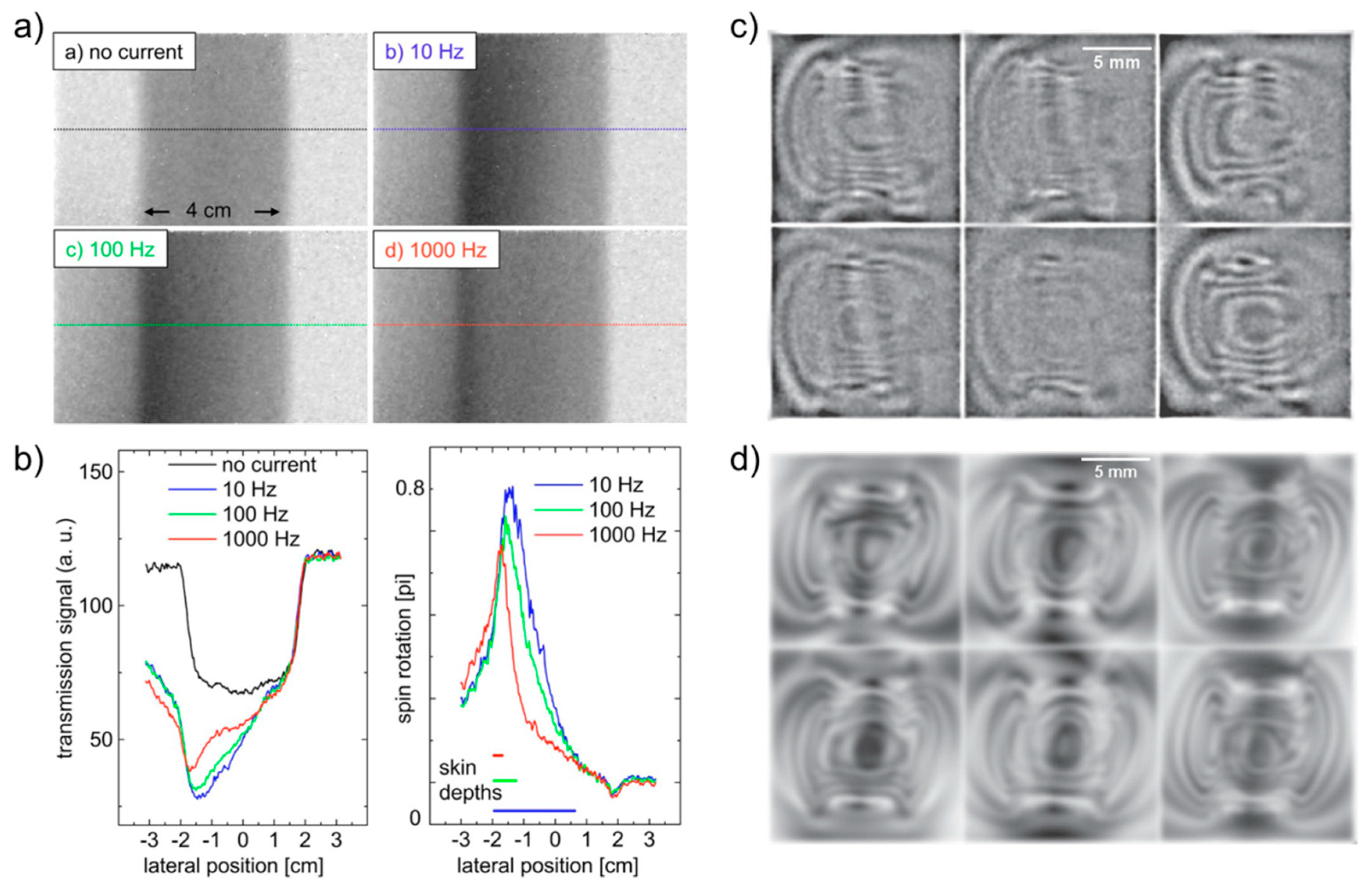
  10. Manke, I.; Kardjilov, N.; Strobl, M.; Hilger, A.; Banhart, J. Investigation of the skin effect in the bulk of electrical conductors with spin-polarized neutron radiography. J. Appl. Phys. 2008, 104, 076109. [Google Scholar] [CrossRef]
  11. Tremsin, A.S.; Kardjilov, N.; Strobl, M.; Manke, I.; Dawson, M.; McPhate, J.B.; Vallerga, J.V.; Siegmund, O.H.W.; Feller, W.B. Imaging of dynamic magnetic fields with spin-polarized neutron beams. New J. Phys. 2015, 17, 043047. [Google Scholar] [CrossRef]
  12. Dawson, M.; Kardjilov, N.; Manke, I.; Hilger, A.; Jullien, D.; Bordenave, F.; Strobl, M.; Jericha, E.; Badurek, G.; Banhart, J. Polarized neutron imaging using helium-3 cells and a polychromatic beam. Nuclear Nucl. Instrum. Methods Phys. Res. Sect. A Accel. Spectrom. Detect. Assoc. Equip. 2011, 651, 140–144. [Google Scholar] [CrossRef]
  13. Michael, S.; Andreas, N.; Sergey, M.; Martin, M.; Elbio, C.; Burkhard, S.; Christian, P.; Peter, B. Towards a tomographic reconstruction of neutron depolarization data. J. Phys. Conf. Ser. 2010, 211, 012025. [Google Scholar]
  14. Dhiman, I.; Ziesche, R.; Wang, T.; Bilheux, H.; Santodonato, L.; Tong, X.; Jiang, C.Y.; Manke, I.; Treimer, W.; Chatterji, T.; et al. Setup for polarized neutron imaging using in situ 3He cells at the Oak Ridge National Laboratory High Flux Isotope Reactor CG-1D beamline. Rev. Sci. Instrum. 2017, 88, 095103. [Google Scholar] [CrossRef] [PubMed]
  15. Sales, M.; Strobl, M.; Shinohara, T.; Tremsin, A.; Kuhn, L.T.; Lionheart, W.R.B.; Desai, N.M.; Dahl, A.B.; Schmidt, S. Three Dimensional Polarimetric Neutron Tomography of Magnetic Fields. arXiv, 2017; arXiv:1704.04887. [Google Scholar]
Figure 1. (a) Schematic diagram of a set-up used for imaging magnetic materials and fields. The neutron beam is polarized, then precesses in a magnetic field, eventually is analyzed and detected. Note that the intensity (dark blue arrow) behind the analyzer is smaller than the intensity behind the polarizer; (b) Field lines surrounding a simple dipole magnet; (c) Radiograph showing field lines around a bar magnet levitating over an yttrium-barium-copper-oxide (YBCO) superconductor as in its superconducting state the YBCO expels all magnetic fields and thus repels the permanent magnet (Meissner effect); (d) Magnetic field trapped in a polycrystalline lead cylinder at different temperatures around Tc = 7.2 K. The trapped flux (yellow regions left and right) inside a polycrystalline cylinder of lead is reconstructed in 3D. When cooled to below its critical temperature in the presence of a weak magnetic field some flux is preserved inside the sample due to defects and grain boundaries and this remains trapped even after the field is switched off [2].
Jimaging 04 00023 g001
Figure 2. (a) Observation of skin effect in a bulk aluminum sample of 4 cm diameter without applied current and with 25 A alternating current at 10 Hz, 100 Hz, and 1000 Hz; (b) Analysis of the spin-polarized image data shows an inhomogeneous magnetic field distribution that can be related to a current distribution similar to this observed in the experiment. The current flows close to the surface of the conductor at high AC frequencies (1 kHz) which is a proof that the skin effect is observed (Reprinted from [10], with the permission of AIP Publishing); (c) Spin-polarized neutron image of magnetic field produced by a 15-loop coil running at 3 kHz current with 10 A rms amplitude measured in a polychromatic neutron beam. The time slice interval of the shown images is 10 µs; (d) Simulations performed based on experimental parameters [11].
Jimaging 04 00023 g002
Figure 3. (a) Comparison between transmission images of a solid-state bender (left) and a polarized 3He spin filter (right) [12]; (b) Mapping of phase transition process from the ferromagnetic to the paramagnetic state of a PdNi crystal (3.24% Ni) using a polarized 3He spin filter setup [13].
Jimaging 04 00023 g003
Figure 4. (a) Example for space discretization used in simulations of imaging with polarized neutrons. (b) Measurements and simulations of spin-precession image of rectangular double coil measured at different current values [3].
Jimaging 04 00023 g004
Figure 5. (a) Polarimetric arrangement for quantitative imaging with polarized neutrons; (b) Measured and simulated spin precession images for different rotation angles of a solenoid for initial spin direction x and analysis of the three orthogonal components of the spin precession angle.
Jimaging 04 00023 g005

