Talking on a Wireless Cellular Device While Driving: Improving the Validity of Crash Odds Ratio Estimates in the SHRP 2 Naturalistic Driving Study


Driving Safety Consulting, LLC, 5086 Dayton Drive, Troy, MI 48085-4026, USA
Safety 2017, 3(4), 28; https://doi.org/10.3390/safety3040028
Submission received: 2 September 2017
/
Revised: 31 October 2017
/
Accepted: 14 November 2017
/
Published: 11 December 2017
(This article belongs to the Special Issue Naturalistic Driving Studies)
Abstract
:Dingus and colleagues (Proc. Nat. Acad. Sci. U.S.A. 2016, 113, 2636–2641) reported a crash odds ratio (OR) estimate of 2.2 with a 95% confidence interval (CI) from 1.6 to 3.1 for hand-held cell phone conversation (hereafter, “Talk”) in the SHRP 2 naturalistic driving database. This estimate is substantially higher than the effect sizes near one in prior real-world and naturalistic driving studies of conversation on wireless cellular devices (whether hand-held, hands-free portable, or hands-free integrated). Two upward biases were discovered in the Dingus study. First, it selected many Talk-exposed drivers who simultaneously performed additional secondary tasks besides Talk but selected Talk-unexposed drivers with no secondary tasks. This “selection bias” was removed by: (1) filtering out records with additional tasks from the Talk-exposed group; or (2) adding records with other tasks to the Talk-unexposed group. Second, it included records with driver behavior errors, a confounding bias that was also removed by filtering out such records. After removing both biases, the Talk OR point estimates declined to below 1, now consistent with prior studies. Pooling the adjusted SHRP 2 Talk OR estimates with prior study effect size estimates to improve precision, the population effect size for wireless cellular conversation while driving is estimated as 0.72 (CI 0.60–0.88).
Keywords:
cell phone; cellular device; wireless; conversation; naturalistic driving; SHRP 2; driving; safety; odds ratio; hands-free; hand-held1. Introduction
Dingus et al. (2016) [1] (hereafter the “Dingus study”) estimated an unadjusted crash odds ratio (OR) for various secondary tasks or task categories, driver behavior errors and driver impairments in an early version 1.0 of the Strategic Highway Research Program Phase 2 (SHRP 2) naturalistic driving study (NDS) dataset [2].
The crash OR estimate is a comparison of the odds of exposure to a risk factor during a crash, to the odds of an exposure to that risk factor during a non-event (e.g., baseline driving without a crash or safety-critical event). The OR estimates the risk ratio (RR) in the general driving population, which is the effect size of interest. Before correction for biases, an OR estimate is known as a “crude” or “uncorrected” estimate; after correction, it is known as an “adjusted” estimate. An adjusted OR point estimate above 1 indicates the risk factor may increase crashes; below 1 it may decrease crashes. (Note: A list of definitions and abbreviations as used in this paper are at the end of the main body.)
In the Dingus study, the crude OR estimate for what it termed “Cell talk (handheld)” (hereafter, “Talk”) was 2.2, with a 95% confidence interval (CI) from 1.6 to 3.1. This Talk OR point estimate is substantially higher and in the opposite direction (i.e., above rather than below 1) compared to the effect sizes (i.e., the RR, rate ratio and OR estimates) of cellular conversation in prior real-world and naturalistic driving studies (see Appendix A). This discrepancy between the Dingus and prior study results raises a question about possible upward biases in the Dingus study Talk OR estimate. To answer this question, the Dingus study Talk OR estimate is first replicated with a new independent analysis of the SHRP 2 database, to verify exactly what analysis methods the Dingus study used to make its Talk OR estimate. The replicated Dingus study analysis methods are then examined for possible biases. Two substantial biases are identified and described. These are each removed in turn and adjusted OR estimates are calculated. Additional potential biases and limitations are noted in the Discussion.
2. Methods
Figure 1 is a flow chart depicting the overall method of the current study, using Talk as an example.
2.1. Step 1: Replicate Dingus Study Talk OR Estimate
After requesting and receiving access to the online SHRP 2 database, Step 1 replicated the Dingus study result for the Talk task as closely as possible. That is, Step 1 queried the SHRP 2 database to determine the crash and baseline counts that best replicated the Talk OR parameter estimates in the Dingus study. This step required an independent analysis of the SHRP 2 database, replicating the analysis and filtering methods as described in the Dingus study. The objective was to reproduce as closely as possible the four specific Dingus study parameters for the Talk task: the Talk OR estimate (2.2); its lower and upper 95% confidence limits (1.6 and 3.1); and the percentage of the randomly-sampled video clips with Talk exposure during balanced-sample baseline driving (3.2%).
2.1.1. Method to Replicate Talk OR Estimate
Four counts of specific database records are required to make an OR estimate for a secondary task such as Talk. These counts form a 2 × 2 table from which the OR estimate is made. Consider the following notation for the distribution of a binary exposure and a crash in a sample of crash and baseline records:
The counts a, b, c, d are of the number of instances of a secondary task occurring (or not) in the database records of 6-s video clip samples. There are two rows with two counts each. The two rows are cases (e.g., all observed crashes) and non-cases (e.g., samples of baseline driving with no safety-relevant event). Using the Dingus study OR estimation method, the two case counts are: a, the number of crash records showing exposure to the secondary task of interest (e.g., Talk); and b, the number of crash records showing no exposure to any secondary task. The ratio of these two counts forms the “case exposure odds,” or a/b. The two counts for the baseline row (i.e., the non-cases or control records) are: c, the number of baseline records showing exposure to the secondary task of interest (e.g., Talk); and d, the number of baseline records showing no exposure to any secondary task. The ratio of these two counts forms the “baseline exposure odds,” or c/d. The ratio of the case and baseline exposure odds is the “exposure OR” estimate, or (a/b) ÷ (c/d) = ad/bc. The exposure OR estimates the risk ratio (RR) in the general driving population, in the absence of bias.
| Exposed | Unexposed | |
|---|---|---|
| Crsah | a | b |
| Baseline | c | d |
The Dingus study did not publish the four record counts a, b, c, d that it used to calculate its Talk OR estimate, or any other OR estimate in that study. The necessary first step in the current study was therefore to replicate the Dingus study Talk OR estimate, in order to determine the counts and analysis methods the Dingus study used to calculate its Talk OR estimate. Based on this Step 1 replication, Steps 2 and 4 then identified biases in those analysis methods and Steps 3 and 5 removed them, giving rise to a final adjusted Talk OR estimate.
The current study uses Talk as an example but the identified biases are present in all the Dingus study OR estimates for secondary tasks and secondary task categories, as shown in Appendix C and Appendix D and discussed in Section 4.4.2.
2.1.2. Confidence Limit Estimation Method
The 95% confidence interval (CI) of the OR estimates were calculated with exact methods using the Stata 13 “cci” command [3]. An exact method is a statistical method based on the actual probability distribution of the study data rather than on an approximation, such as a normal distribution. It is commonly recommended in Epidemiology to use an exact solution when any count in the 2 × 2 table is less than about 10; if all counts are higher than that, the exact and inexact methods give rise to similar CIs. Slight differences in the exact confidence limits calculated in the current study replication (compared to the Dingus study confidence limits) may arise because the Dingus study did not report that it used an exact solution. In addition, there were likely some slight differences in the counts found in the current replication compared to what the Dingus study may have used (for reasons noted in Section 2.1.9), and these differences could also affect the confidence limit estimates.
2.1.3. Database Versions and Tabulation Method for Crashes
As mentioned, the Dingus study [1] used an early version 1.0 of the SHRP 2 database [2] that was available at the time. This version has been superseded by several later versions. The current study replicated the Dingus study OR estimates for secondary tasks as closely as possible using version 2.1.1 of the SHRP 2 database [6] that was available at the time of the current study.
The tabulations in this paper have been updated from those in a previous conference technical paper (Young, 2017a) [7] that were based on the prior SHRP 2 database version 2.0.0, so there are some slight differences in some record counts.
The counts of SHRP 2 crash events with secondary tasks were tabulated using the Query system provided at the InSight website [6], which provides internet access to the database for qualified researchers. Secondary task occurrences associated with crashes were defined by the Virginia Tech Transportation Institute (VTTI) in a “case window,” which was 5 s prior to and 1 s after, a “precipitating event” before the crash.
In a few instances, the first crash was immediately followed by a second crash. In a few other instances, there was a non-crash (such as a near-crash) recorded as the first event, which was then immediately followed by a crash. The Dingus study does not specify how it handled such dual-event instances. However, it seemed implausible that a secondary task that occurred before the first event could have a direct causal relationship with a second event. It is more plausible that the first safety-related event would capture the driver’s attention and the second event was more related to driver control issues arising from the first event, rather than to a secondary task that occurred prior to the first event. As a check, the current analyses were redone counting all crashes (i.e., both first and second crashes, if any). There was little difference in the results, so only the crash events that first occurred in a sequence are reported here.
The Dingus study states that it tabulated only “injurious and property damage” crashes and it was assumed in the current study that these were crashes of severity levels I–III, so these were tabulated here. The severity levels are defined in the SHRP 2 database information comments as: I (severe, an airbag/injury/rollover/high delta-V crash that is almost always police reported); II (property damage, including police-reported crashes and others of similar severity that were not police-reported); and III (minor, crashes involving physical contact with another object). Level IV crashes were “minor” tire strikes and were not included in the Dingus or current study.
The assumption that the Dingus study used only severity levels I–III was verified because the total number of crashes of severities I–III in the SHRP 2 version 2.1.1 database was 834, which was close to the total number of crashes reported by the Dingus study of 905. The most plausible reason for 71 (7.8%) more total crashes in the Dingus study than in the current version 2.1.1 of the SHRP 2 database is because of changes in the database from version 1.0 [2] used by the Dingus study to version 2.1.1 [6] at the time of the current study. This discrepancy in the total crash count does not affect the identified biases in the Dingus study, nor their adjustments, for reasons given in Section 2.1.9.
2.1.4. Tabulation Method for Balanced-Sample Baseline Records
To form the balanced-sample baseline dataset, the VTTI video reductionists randomly selected records from each driver’s videos, such that the number of baseline record samples for each driver was proportional to that particular driver’s total driving time over 5 mph while the ignition was on during the SHRP 2 study period. The VTTI video reductionists placed the records resulting from that sampling procedure into the baseline database records for that driver.
For the control (baseline) dataset without a safety-critical event, the SHRP 2 balanced-sample baseline database had 19,998 records in database version 2.1.1. This balanced-sample baseline was used for the current analysis, replicating the Dingus study methods. The Dingus study reported it had 19,732 balanced-sample baseline records in database version 1.0, or 266 fewer records than the 19,998 in the SHRP 2 database version 2.1.1. The reason for this 1.3% discrepancy is not determinable from the information in the published Dingus paper but it is again likely because of the different database versions. This discrepancy in the total baseline count also does not affect the identified biases in the Dingus study, nor their adjustments, again for reasons given in Section 2.1.9.
2.1.5. Tabulation Method for Secondary Tasks
There was a 6-s time window for counting secondary tasks in both crash and baseline video clips. Note that the “anchor point” for crashes was the time of the precipitating event, not the crash time. The case window used by the video reductionists for tabulating secondary tasks in the case database was then 5 s prior to and 1 s after this precipitating event anchor point.
Although the baseline control video clips were 20 s or more in duration, secondary tasks were tabulated for only the last 6 s. VTTI (2015) [8] (p. 6) states, “The anchor point for baselines is defined to occur one (1) second prior to the end (last timestamp) of the baseline epoch”. In other words, the baseline window employed by the video reductionists for tabulating secondary tasks in the baseline database was 5 s prior to and 1 s after, this anchor point.
In the online SHRP 2 database for crashes and baselines, there were up to 3 “slots” (i.e., fields or variables in a given database record) that could be filled with up to 3 secondary task types, if any, as observed by the VTTI video reductionists in the 6-s video samples. That is, either 0, 1, 2, or 3 of these secondary task slots could be filled with a secondary task name that was observed in a particular 6-s case or control sample window.
The start and end times of the secondary tasks (up to the limits of the 6-s window) were given in the database for the crash cases (but not the baseline controls). It can be deduced from these start and end times that most of the secondary tasks in a given record were simultaneously performed (i.e., multi-tasked) during the 6-s case window (e.g., conversing on a cell phone while adjusting an in-vehicle device), while some others were sequentially performed (e.g., ending one call and then dialing another).
2.1.6. Tabulation Method for Driver Behavior Errors
There are 69 separate and distinct types of “driver behavior errors” in the SHRP 2 version 2.1.1 dataset, along with operational definitions suitable for coding of each error when observed by VTTI video reductionists (VTTI, 2015) [8] (pp. 49–54). The entire list and definitions of these 69 driver behavior errors need not be presented here. Note that these definitions were empirical, based on observations of the driver behavior errors in the videos and they did not conform to nor were they based on any particular theory or model of driver errors, on which there is an extensive literature. Rather than individually analyzing each of these 69 driver behavior error types, the Dingus study summed many of them a priori into various categories and sub-categories it created.
The first major driver behavior error category in the Dingus study was “Driver Performance Error”. It was operationally defined [1] (p. 2636) as the sum of “driver performance error, including a variety of vehicle operation and maneuver errors (e.g., failing to yield properly to other traffic, making an improper turn)”. This category had an overall baseline prevalence of 4.81%. There were 10 major error subcategories observed in crash and baseline events in this “Driver Performance Error” category. “Failed to signal” had the largest baseline prevalence at 2.27%; “Stop/yield sign violation” was next highest at 1.05%; “Driving too slowly” was third-highest at 0.97%; and “Improper turn” was fourth-highest at 0.51% baseline prevalence.
The second major driver behavior error category in the Dingus study was “Driver Momentary Judgment Error (Speeding/Aggressive Driving)”. This category was operationally defined by the Dingus study [1] (p. 2636) as “momentary driver judgment error, including such factors as aggressive driving and speeding”. It had an overall baseline prevalence of 4.22%. There were 7 major error subcategories observed in crash and baseline events in this category. “Speeding (over limit and too fast for conditions” had the largest baseline prevalence at 2.77%; “Intentional stop/yield sign violation” was next highest at 1.04%; “Intentional signal violation” was third-highest at 0.19%; and “Illegal/unsafe passing” was fourth-highest at 0.18% baseline prevalence.
There were 3 “slots” or variables in the SHRP 2 crash and balanced-sample baseline database records that could each be filled with a driver behavior error if observed in the same 6-s video clip used to record secondary tasks. However, identification of driver behavior errors in that 6-s video window was enhanced by looking at the video file up to 20 s before the precipitating event.
These three driver behavior error variables were entirely separate from the three secondary task variables. The exception is an entry of “Distraction” in the first driver behavior error variable that was present for many records in the crash database but not in the baseline database. These “Distraction” entries were historically in the database simply to indicate that a secondary task was present in the case window before a crash. It does not mean that “Distraction” is a driver behavior error, nor was it not counted as such in either the Dingus study or the current study.
2.1.7. Impairments
The Dingus study (2016) [1] (p. 2637) states, “As impairment typically has a higher safety impact than distraction, impairment was excluded from the distraction assessment”. That is, the Dingus study filtered out all records containing a driver impairment from both the Exposed and Unexposed variables for both crashes and baselines, before calculating its secondary task OR estimates. Therefore, the current study also filtered out records with noticeable driver impairment from drugs, alcohol, drowsiness, etc., in its queries of the online SHRP 2 version 2.1.1 crash and baseline databases. Note that driver impairments were tabulated in the databases based on a 20-s window, rather than the 6-s window for secondary tasks and driver behavior errors, because it is difficult to identify impairments such as drowsy driving in short time windows (Ahlstrom et al., 2015) [9].
In the SHRP 2 crash database version 2.1.1, there were 58 out of 834 (7.0%) crash records of severities I–III with observable driver impairment. Filtering out crash records with driver impairment left 776 crash records of severities I–III without observable driver impairment in the current study.
In the SHRP 2 balanced-sample baseline database version 2.1.1, there were 381 out of 19,998 (1.9%) balanced-sample baseline records with observable driver impairment. The current study also filtered out all baseline records with impairment, leaving 19,617 balanced-sample baseline records without observable driver impairment in the current study.
In short, records with a driver impairment were filtered out of all cells in all Tables in the main body of this paper, replicating the impairment filtering method stated in the Dingus study.
Because all records containing a driver impairment were filtered out, driver impairments could not have biased the Talk OR estimates in either the Dingus or current study. Therefore, driver impairments are not considered further in the current paper.
2.1.8. “Model Driving”
The Dingus study defines its term “Model Driving” for crashes and baselines simply as “alert, attentive and sober” [1] (p. 2637). It is not explicitly stated in the Dingus study methods what was meant by those terms operationally. Indeed, the terms “alert” “attentive” and “sober” are not in the SHRP 2 database records. It was therefore assumed that by the word “alert” that the Dingus study meant that it filtered out all crash and baseline records with “drowsiness”. Likewise, it is assumed from the word “sober” that the Dingus study filtered out all records with observable drug or alcohol impairments. It is suggested by the word “attentive” that the Dingus study filtered out all records with a secondary task from its “Model Driving” counts of crash and baseline records; however, this is not explicitly stated in the Dingus study methods.
It is also not explicitly stated in the Dingus study methods whether or not video clips with driver behavior errors were or were not filtered out from its “Model Driving” definition, or from its crash cases. Therefore, OR estimates were calculated in the current study with and without filtering of driver behavior errors from “Model Driving” and crash cases. The “additional secondary task” and “driver behavior error” conditions that gave rise to the closest match to the Dingus study parameters for its Talk OR estimate are reported in the Step 1 replication in Section 3.1.
2.1.9. Database Issues and Workarounds
The Step 1 replication found only minor differences between the replicated and the original Dingus study results [1]. There were small differences in the total crash record counts as described in Section 2.1.3 and small differences in the total baseline record counts as described in Section 2.1.4. These differences were found in the Step 1 replication, before the bias adjustments in the Dingus study analysis methods in Steps 3 and 5.
A few of these differences were traced to bugs in the InSight Query program or in the SHRP 2 database itself, all of which were immediately reported to and fixed by, the Virginia Tech Transportation Institute (VTTI) Query database group, during the course of the current study. All results reported here are after correction of these bugs. However, several minor differences still remained in the crash and baseline record counts after correction of these bugs, as noted in the previous Section 2.1.3 and Section 2.1.4 for crash and baseline counts respectively.
The major reason for these minor differences was again likely because of the differences in the early version 1 of the SHRP 2 database [2] at the time of the Dingus study, compared to the SHRP 2 version 2.1.1 database update, released in May 2016 [6] and used for the current study. For example, the change descriptions in the database versions indicate that a number of crashes and baseline records were removed in version 2.1.1 compared to earlier versions because of privacy or consent issues, or driver ID corrections.
Regardless, these differences are immaterial to the main findings of the current study, which have to do with biases in the Dingus study analysis methods and their adjustment. Analysis biases affect any and all OR estimates regardless of the SHRP 2 database version. In other words, the differences between database versions are without consequence for the results and conclusions of the current study, because the biases found in the Dingus study were in the analysis methods it employed, which would bias the OR estimates no matter what data were in any particular version of the SHRP 2 database. In short, any small discrepancies in whatever counts the Dingus study may have used and the counts in the current study are immaterial to the main findings of the current study, which concern biases in the Dingus study analysis methods, rather than in the SHRP 2 database records themselves.
In summary of Step 1, various attempts were made to query the SHRP 2 database, using different assumptions about whether additional secondary tasks were or were not present and whether driver behavior errors were (or were not) present in the Talk-exposed and Talk-unexposed crash and baseline records that the Dingus study selected to analyze. The crash and baseline counts so found were placed into standard 2 × 2 matrices for calculating OR estimates (Rothman, 2012) [10] (pp. 87–102). The 2 × 2 matrix that most closely approximated the four Dingus study Talk parameters (the OR estimate, its upper and lower confidence limits and the % baseline prevalence exposure) was judged to be the correct replication.
2.2. Steps 2 and 4: Identify Selection and Confounding Biases
Once the counts were approximated in the Step 1 replication, Steps 2 and 4 could then easily determine whether biases were present in the Dingus study analysis methods. In particular, once the four record counts were known (the Talk-exposed and Talk-unexposed crash and baseline record counts), the biases could be easily identified and illustrated using standard 2 × 2 tables, applying standard epidemiological stratification and analysis methods. In other words, Step 2 involved an analysis of the filtering methods in the queries used to generate the replicated 2 × 2 Talk matrix, to identify possible biases in the analysis methods used in the Dingus study. If the replicated count tabulations in Step 1 revealed major biases in the analysis methods used to generate them, then it is plausible that these biases were likely present in the Dingus study as well.
2.3. Steps 3 and 5: Remove Biases, Final Adjusted OR Estimate
Once Steps 2 and 4 identified the biases, Steps 3 and 5 then removed those biases. Step 3 used two different methods of bias removal to provide an independent check. After Step 5, two adjusted Talk OR estimates were the final output, with the two major identified biases removed. There were two methods of “additional secondary task” bias removal in Step 3, so there were two final adjusted OR estimates.
These final adjusted Talk OR estimates have improved validity over the original Dingus study estimate because of bias removal. However, they are still not necessarily valid estimates of the population Talk risk ratio, because additional biases are likely still present, as noted in the Discussion Limitations Section 4.5.
2.4. Overall Summary of 2 × 2 Table Designs
A series of six 2 × 2 tables were designed with various combinations of additional tasks and driver behavior errors being present or not in the Talk-exposed and Talk-unexposed (or “Not Talk”) columns to accomplish Steps 1–6 in the procedure illustrated in Figure 1.
3. Results
3.1. Step 1: Replicate Dingus Study Talk OR Estimate
Table 1 is a 2 × 2 tabulation of the crash and baseline records in the SHRP 2 database that best replicated the Dingus study Talk OR estimate, confidence limits and the percentage of Talk-exposed baseline records.
In the Exposed column in Table 1, the notation for the superscripts “a” and “b” for Talkab indicate the following: “a” indicates “additional” —Talk was not always the only secondary task in the 6-s record and could be accompanied by up to 2 additional secondary tasks; “b” indicates “behavior” — 0 to 3 driver behavior errors could be present in the same record as Talk.
In the Unexposed column in Table 1 (what the Dingus study called “Model Driving”), the notation for the superscripts “0” and “b” for Not Talk0b indicate the following: “0” indicates that 0 secondary tasks were present in the 6-s record; “b” indicates “behavior” — 0 to 3 driver behavior errors could be present in the record without Talk.
The Table 1 Talkab OR estimate of 2.2 (CI 1.5–3.2) closely replicated the Dingus study Talkab OR estimate of 2.2 (CI 1.6–3.1). In addition, the prevalence of Talkab (i.e., percentage of the total balanced-sample baseline records exposed to Talkab) was replicated at 3.2%. Thus, the replication was successful, because compared to the four Dingus study parameters, the replication has: (1) the same Talkab OR estimate to the first decimal place; (2) the same percentage of the total balanced-sample baseline records exposed to Talkab to the first decimal place; and (3) only a 0.1 difference in the first decimal place in the confidence limits. This slight difference is likely because the current study used SHRP 2 database version 2.1.1, which likely had slightly different records from the Dingus study SHRP 2 version 1.0, as noted in Section 2.1.9. As a result of these close similarities in the four Talk parameters, the replicated and Dingus study Talkab OR estimates have a p for homogeneity near 1.
From this successful Table 1 replication of the Dingus study Talkab OR estimate parameters, Steps 2 and 4 readily identified two major biases. The main objective was to find out if these biases help explain why the Dingus study Talkab OR estimate is biased upwards compared to prior epidemiological studies of Talk effect sizes, as shown in Appendix A.
Detailed definitions and evidence for the upward biasing effect of these two biases on the Talk OR estimate are presented in the following sections. As per the flow diagram in Figure 1, Step 2 (Section 3.2.1) identifies the selection bias and Step 3 (Section 3.2.2 and Section 3.2.3) gives two equivalent methods of removing selection bias from the OR estimate. Step 4 (Section 3.3.1) identifies a confounding bias from driver behavior errors and Step 5 (Section 3.3.2 and Section 3.3.3) removes this confounding bias from the two OR estimates from Step 3. The adjusted Talk OR estimates with both biases removed are then the final output.
3.2. Selection Bias from Additional Secondary Tasks
3.2.1. Step 2. Identify Selection Bias
Selection bias is a formal term in epidemiology which refers to a distortion in the effect size estimate that results from the procedures used to select subjects. A formal epidemiological definition of selection bias is given by Porta (2014) [11] (p. 258): “Bias in the estimated association or effect of an exposure on an outcome that arises from the procedures used to select individuals into the study or the analysis”.
The first major analysis bias identified in the replication is selection bias from additional secondary tasks. It is illustrated in the row in Table 1 labelled “Additional secondary tasks”. This bias occurs because there were additional secondary tasks in the Exposed but not Unexposed column. The Exposed column tabulates the database records of video clips which show the driver was Talkab-exposed. The Unexposed column tabulates the database records of video clips with Not Talk0b. Using different criteria for the Exposed and Unexposed columns is a classic example of selection bias.
In other words, the replication revealed that selection bias was present in the Dingus study analysis methods because its criterion for selecting its Talk-exposed records (with additional secondary tasks) was not the same as its criterion for selecting Talk-unexposed records (without additional secondary tasks). The current paper labels this additional task selection bias, because it arises from the differential selection criterion that the replication found that the Dingus study used for additional tasks for the Talk-exposed vs. Talk-unexposed drivers.
The details of this “additional task selection bias” in the Table 1 replication are seen in a close examination of the four cells in the 2 × 2 Table 1 matrix:
- Upper left cell, note w. Of the 34 Talkab crash cases, note w shows that 18 of those cases (53%) had additional exposure to secondary tasks besides Talk in the same 6-s exposure window as Talk. There were actually 22 additional tasks, because four of the records with Talk contained two additional secondary tasks besides Talk; i.e., the driver was triple-tasking. Only 9 of those 22 additional tasks were visual-manual tasks associated with the hand-held cell phone used for Talk, such as browsing, dialing, holding, locating/reaching/answering, or texting.
- Upper right cell, note x. There were 776 records without Talk exposure (Not Talk0b) in the 6-s case window, after which the driver crashed. The Dingus study methods section states that it purposefully selected only those Talk-unexposed cases with no secondary tasks at all (what it termed “Model Driving”), which the replication found occurred in only 235 (30%) of the total 776 crash cases.
- Lower left cell, note y. There were 626 records with exposure to Talkab in the 19,617 total unimpaired balanced-sample baseline control records without any safety-critical event (3.2% baseline prevalence, note e). Note y shows that 92 (15%) of these 626 baseline records contained exposure to additional secondary tasks besides Talk.
- Lower right cell, note z. There were 18,991 records without Talk exposure (Not Talk0b) in the 19,617 total unimpaired balanced-sample baseline control records without any safety-critical event. From those 18,991 records, the Dingus study purposefully selected only the 9,420 baseline controls with no secondary tasks at all.
Therefore, the left column of Table 1 (Talkab) tabulates counts not just of the records with exposure to Talk but also with exposure to additional secondary tasks besides Talk. (There is also exposure to driver behavior errors here as well, as later discussed in Section 3.3.)
On the other hand, the right column (Not Talk0b), tabulates counts only of those records which were deliberately selected by the Dingus study to have no secondary tasks at all—what the Dingus study terms Model Driving.
In other words, selection bias occurs because additional secondary tasks were present in the Talk-exposed counts (i.e., the Talkab records) but not in the Talk-unexposed counts (i.e., the Not Talk0b records). That is, the majority of the video clips with exposure to Talk and in which the driver crashed, contained concurrent exposure to additional secondary tasks besides Talk in the 6-s exposure window surrounding the precipitating event before the crash. The Dingus study analysis method exhibits selection bias because it contrasted these Talk-exposed record counts not just with the record counts of video clips without Talk exposure but a specific subsample of the Talk-unexposed records; namely, only those records in which a driver performed no secondary tasks at all.
3.2.2. Step 3. Method 1 to Remove Selection Bias: Talk0b
The first method to remove the “additional task” selection bias in the Table 1 replication was to filter out all those Talk-exposed drivers from the Exposed column of Table 1 who were multi-tasking with additional secondary tasks besides Talk in the same 6-s exposure window. This filtering creates Talk0b (i.e., Talk with no additional secondary tasks but with driver behavior errors). Selection bias is removed, because the drivers in both the Exposed and Unexposed columns now do not have exposure to secondary tasks other than Talk. Table 2 is the 2 × 2 matrix showing the adjusted OR estimate for Talk0b without “additional task” selection bias. Key changes in exposure conditions and cell counts from Table 1 are marked in italics.
Table 2 gives rise to a Talk0b OR point estimate of 1.2, a 45% reduction from the Dingus study Talkab OR point estimate of 2.2 in Table 1. This result demonstrates that selection bias almost doubled the Talk0b OR point estimate from 1.2 in Table 2, to the Talkab OR point estimate of 2.2 in Table 1.
This false elevation of the Dingus study Talkab OR estimate from the “additional task” selection bias was confirmed by calculating the TalkAb OR estimate for the complement of the Talk0b Exposed column in Table 2. The complement was formed from the stratum of Talk-exposed cases in Table 1 that always had additional secondary tasks; i.e., the database records that were filtered out from Table 1 to form Table 2.
In Table 3, drivers in the “Exposed” column are now always double- or triple-tasking Talk with other secondary tasks in one 6-s video clip, or TalkAb (the superscript A denoting Always). Key changes from Table 1 in exposure conditions and cell counts are again marked in italics.
Table 3 shows that this TalkAb OR estimate elevates to a substantial 7.8 (CI 4.4–13.3) when video clips always show the driver multi-tasking with additional secondary tasks during Talk, again compared with Not Talk0b with no secondary tasks. The resulting high TalkAb OR point estimate of 7.8 provides strong evidence that the additional secondary tasks in the Table 1 Exposed column caused a substantial upward bias in the replicated Dingus study Talkab OR estimate.
However, Talk0b and TalkAb in Table 2 and Table 3 respectively should not even be summed together to form the Talkab exposure in Table 1, as was implicitly done by the Dingus study. A homogeneity test of the OR estimates in Table 2 and Table 3 finds that the p-value testing homogeneity between these two strata is p < 0.0000001, indicating substantial heterogeneity between the Table 2 Talk OR0b estimate of 1.2 (CI 0.7–2.0) and the Table 3 TalkAb OR estimate of 7.8 (CI 4.4–13.3). One can therefore conclude with a high degree of confidence that the effect size (i.e., the OR estimate) is not constant across Table 2 and Table 3. Because the data do not conform to the assumption that the effect size is constant across strata, the strata must not be pooled (Rothman, 2012) [10] (p. 178). In other words, it is misleading (and technically incorrect) to represent the Talkab OR estimate of 2.2 in Table 1 as the valid estimate for the Talk crash risk ratio for the population, because it is composed of two heterogeneous effects: Talk always with additional tasks (Table 3) and Talk with no additional tasks (Table 2). Heterogeneity means that the Talk0b OR estimate of 1.2 (CI 0.7–2.0) and the TalkAb OR estimate of 7.8 (CI 4.4–13.3), must be separately analyzed and reported as per Table 2 and Table 3 and not pooled to create Table 1 (Rothman, 2012) [10] (p. 178) as was implicitly done by the Dingus study.
3.2.3. Step 3. Method 2 to Remove Selection Bias: Retain Other Secondary Tasks in Unexposed Group
A second method to remove the “additional task” selection bias in Table 1 is by selecting drivers with secondary tasks other than Talk in both the Exposed and Unexposed columns. The Exposed and Unexposed columns are then again balanced for tasks other than Talk, as they were in Table 2. In other words, balance is achieved when the Exposed and Unexposed columns are equal in their selection criteria. In Table 2, neither column had additional secondary tasks; in Table 3, both do.
Table 4 illustrates this second method. Key changes from Table 1 in exposure conditions and cell counts are again marked in italics.
Table 4 is unlike the replicated Dingus study analysis in Table 1 because it allows other secondary tasks besides Talk in the Unexposed column. The balance in the selection criteria for the Exposed and Unexposed columns again removes the “additional task selection bias” from the Table 1 Talkab OR estimate. In Table 4 the Exposed and Unexposed columns are balanced because they both included secondary tasks other than Talk. In Table 2 the columns are balanced because they both did not include secondary tasks other than Talk.
Table 4 calculates a Talkab OR estimate of 1.4 (CI 0.95–2.0). This Talkab OR estimate is homogeneous with the Table 2 Talk0b OR estimate of 1.2 (CI 0.67–2.0) with p for homogeneity = 0.65. In other words, either method of eliminating selection bias reduces the replicated Talkab OR estimate of 2.2 (CI 1.5–3.2) in Table 1 to about the same effect size: 1.2 (CI 0.67–2.0) in Table 2 and 1.4 (CI 0.95–2.0) in Table 4.
Note that Table 2 and Table 4 have different Talk-unexposed columns: the Table 2 Talk-unexposed column (Not Talk0b or “No Task”) has no exposure to any secondary task, whereas the Table 4 Talk-unexposed column (Not Talkab) has exposure to many secondary tasks other than Talk. The homogeneity in the Table 2 and Table 4 OR estimates indicates that the two unexposed methods are equally successful at eliminating selection bias, as long as the Exposed column is equal and balanced with the Unexposed column. Hence, the Table 2 Talk-exposed column (Talk0b) must have Talk by itself, with no exposures to any additional secondary tasks, whereas the Table 4 Talk-exposed column (Talkab) must have exposure to secondary tasks other than Talk.
However, the Table 4 Unexposed column “No Talk” method has some technical advantages over the Table 2 Unexposed column “No Task” method used in the Dingus study. First, it is more like common everyday driving, because the SHRP 2 drivers typically performed other secondary tasks in about 50% of baseline video clip samples without exposure to Talk (note z in Table 4). Second, Table 4 has a larger n in all four cells of the 2 × 2 matrix compared to Table 2 because the secondary tasks other than Talk were present in all four cells. This larger n improves the precision of the Talk OR estimate—the confidence interval is improved (i.e., reduced) from 1.33 (2.0 − 0.67) in Table 2 to 1.05 (2.0 − 0.95) in Table 4. The Table 4 method is also the standard epidemiological method, which evaluates the complement of the risk factor under investigation in the Unexposed column (i.e., Talk vs. Not Talk).
However, the Table 4 method may have a slight disadvantage over the Table 2 method because of a potential confounding bias (see Section 3.3.1) because secondary tasks other than Talk are now present in both the Exposed and Unexposed columns. Yet, as previously noted, the OR estimates in Table 2 and Table 4 are homogeneous, indicating that the potential confounding bias from other secondary tasks being present in both the Exposed and Unexposed columns is negligible.
3.3. Confounding Bias from Driver Behavior Errors
A second major bias was suspected of still being present after removal of the selection bias described in Section 3.2. The reason for this suspicion is that the Table 2 and Table 4 OR point estimates of 1.2 and 1.4, although reduced from the Dingus study OR point estimate of 2.2, were still both above 1. That is, these OR point estimates are still higher and in the opposite direction (i.e., above rather than below 1) compared to the prior real-world and naturalistic driving point effect sizes listed in Appendix A. This discrepancy raises the question of whether other upward biases are still present in the Talk OR estimates in Table 2 and Table 4.
3.3.1. Step 4: Identify Confounding Bias
A potential second bias is illustrated in the row labelled “Driver behavior errors” in Table 1, Table 2, Table 3 and Table 4. A confounding bias may arise from the fact that driver behavior errors were present in both the Exposed and Unexposed columns in Table 1, Table 2, Table 3 and Table 4. A formal definition of confounding bias is given in Appendix B, with evidence that driver behavior errors meet this formal definition.
It is not explicit in the Dingus study methods section whether driver behavior errors were removed or not before it made its secondary task OR estimates. However, the Table 1 replication revealed that all four cells in the 2 × 2 matrix contained varying percentages of records with driver behavior errors. Specifically, the Table 1 notes show that the following driver behavior error percentages were present in each of the four cells in the Table 1 2 × 2 matrix:
- Upper left cell, Talkab-exposed cases, note w. Of the 34 crash cases with exposure to Talkab, 23 (68%) contained driver behavior errors: 15 single (44%), 7 double (21%) and 1 triple (3%) driver behavior error. There was thus a remarkable total of 32 driver behavior errors present in the 34 Talkab-exposed crash case records. The most common driver behavior error was “improper turn, cut corner” with 12 records (8 with single and 4 with double driver behavior errors).
- Upper right cell, Not Talk0b Unexposed cases, note x. Of the 235 crash case records with no secondary tasks, 141 (60%) contained driver behavior errors: 103 single (44%), 28 double (12%) and 10 triple (4%), for a total of 189 driver behavior errors in 235 Unexposed crash cases. The most common error was “Exceeded safe speed but not speed limit” in 33 crash case records (21 single, 11 double, 1 triple error). The fact that 60% of the drivers in this Not Talk0b case column engaged in driver behavior errors, raises the question of whether the Dingus study term “Model Driving” for the Unexposed column is misleading.
- Lower left cell, Talkab-exposed baselines, note y. Of the 626 baseline records with exposure to Talk, 54 records (9%) had driver behavior errors: 51 single (8%), 3 double (0.5%) and 0 triple (0%). The total is 57 driver behavior errors in 626 baseline control records. The most common error was “Exceeded speed limit”.
- Lower right cell, Not Talk0b Unexposed baselines, note z. Of the 9,420 baseline control records with no secondary tasks, 778 records (8%) had driver behavior errors: 694 single (7%), 75 double (0.8%) and 9 triple (0.1%), for a total of 871 driver behavior errors in 9,420 baseline control records. The most common error was again “Exceeded speed limit” as in the lower left cell. The fact that 8% of the drivers in this Not Talk0b baseline cell had driver behavior errors, again raises the question of whether the Dingus study term “Model Driving” for the Unexposed column is misleading.
In short, the Table 1 replication revealed that the Dingus study methods did not filter out records with driver behavior errors in any of the four 2 × 2 cell entries in Table 1—the Exposed and Unexposed crash cases and the Exposed and Unexposed baseline controls. This bias is not a selection bias, because both the Exposed and Unexposed columns had the same selection criterion for driver behavior errors; that is, they did not filter out such errors. However, this bias potentially meets the formal definition of confounding bias for driver behavior errors as shown in Appendix B.
3.3.2. Step 5.1. Remove “Driver Behavior Error” Confounding Bias from Table 2
In Step 5.1, any potential confounding of the Talk OR estimate by driver behavior errors in Table 2 is removed by simply filtering out all records with driver behavior errors. Table 5 gives the 2 × 2 matrix for the Talk OR estimate after removing all records containing driver behavior errors from Table 2, which had already removed “additional task” selection bias. Key changes from Table 1 in exposure conditions and cell counts are again marked in italics.
Table 5 has what may now be called “Pure Talk” for the Exposed column, because Talk00 has no driver behavior errors and no additional secondary tasks. That is, in Table 5, the Exposed cases and controls have only Talk, unlike the Dingus study replication in Table 1, which can have additional tasks and driver behavior errors in the same 6-s exposure window with Talk. Likewise, Table 5 has what may now be called “Pure Driving” for the Not Talk00 Unexposed column, because it has no driver behavior errors and no secondary tasks.
Table 5 shows that after removing driver behavior errors from the Exposed column of Talk0b and the Unexposed column of Not Talk0b in Table 2, the Talk OR0b estimate declines from 1.2 (CI 0.67–2.0) in Table 2 to the Talk00 OR estimate of 0.94 (CI 0.30–2.3) in Table 5, a further 23% decline beyond that after removal of the additional task selection bias given in Table 2. This further decline indicates that the confounding from “driver behavior error bias” also falsely elevated the Talkab OR point estimate in the Dingus study, as did the “additional task” selection bias. The 23% decline sums with the 45% decline in Table 2, for a total decline of 68% for the Talk00 OR point estimate of 0.94 in Table 5, compared to the replicated Dingus study Talkab OR point estimate of 2.2 in Table 1.
3.3.3. Step 5.2. Remove “Driver Behavior Error” Confounding Bias from Table 4
In Step 5.2, any potential confounding of the Talkab OR estimate by driver behavior errors in Table 4 is removed by filtering out all records containing driver behavior errors. Table 6 gives the 2 × 2 matrix for the Talka0 OR estimate after removing the “driver behavior error” records from Table 4, which had already removed records to eliminate “additional task” selection bias. Hence this method removes both driver behavior error bias and additional task selection bias, as did Table 5.
Table 6 gives the result of removing the driver behavior error confounding bias from Table 4. Key changes in exposure conditions and cell counts from Table 1 are again marked in italics.
Table 6 has what is here termed Talka0 for the Exposed column, because records containing driver behavior errors have been removed from the Table 4 Exposed column of Talkab. That is, in Table 6, the term Talka0 for the Exposed column means it has Talk plus additional secondary tasks (superscript “a”) but no driver behavior errors (superscript “0”). Likewise, the term Not Talka0 for the Unexposed column means it does not have records containing Talk but it does have records containing other secondary tasks (superscript “a”) but not driver behavior errors (superscript “0”).
Table 6 demonstrates that filtering out driver behavior errors from both the Exposed and Unexposed columns reduces the Table 4 Talkab OR estimate with driver behavior errors of 1.4 (CI 0.95–2.0), to the Table 6 Talka0 OR Estimate without driver behaviors to 0.92 (CI 0.45–1.7).
The Table 5 Talk00 OR estimate of 0.94 (CI 0.30–2.3) and the Table 6 Talka0 OR estimate of 0.92 (CI 0.45–1.7) are homogeneous with p = 0.96, meaning both methods were equally successful in removing the two identified biases from the Dingus study replication in Table 1. These OR estimates are also homogeneous with the RR, rate ratio and OR estimates in prior real world and naturalistic driving studies listed (see Appendix A).
The Table 6 method for removing the confounding bias has an advantage over the Table 5 method because it has a larger n in every cell of the 2 × 2 matrix, due to the secondary tasks other than Talk in the Exposed and Unexposed columns. The larger n improves the precision of the OR estimate—the confidence interval is improved (i.e., reduced) from 2 (2.3 − 0.3) in Table 5 to 1.25 (1.7 − 0.45) in Table 6.
On the other hand, the Table 6 method has a possible disadvantage over the Table 5 method because it has a new potential confounding bias from the other secondary tasks in both the exposed and unexposed cases. However, the homogeneity (p = 0.96) of the OR estimates in Table 5 and Table 6 provides substantial evidence that this potential confounding bias from other secondary tasks is negligible.
3.4. Summary of Overall Design and Talk OR Estimates for Table 1, Table 2, Table 3, Table 4, Table 5 and Table 6
Table 7 summarizes the overall study design for Table 1, Table 2, Table 3, Table 4, Table 5 and Table 6 with the OR estimates for each.
The second column of Table 7 lists the purpose of each Table 1–6. The third column gives the Talk-exposed variable name. The fourth column is the number of possible additional tasks that could be tabulated in the same single database record as Talk, ranging from 0 to 2. The fifth column is the number of driver behavior errors that could be tabulated in a Talk record, ranging from 0 to 3. The next three columns have the same variable names as the previous three columns but for Talk-unexposed records; i.e., those in the Not Talk or Unexposed column. The last four columns give the OR estimates, lower (LL) and upper (UL) confidence limits, and the p-values for the OR estimates in the six Tables.
The main study objective was to determine why the Dingus study had an elevated Talkab OR estimate of 2.2 (CI 1.6–3.1), compared to the prior real-world and naturalistic driving studies in Appendix A, which all had Talk point effect sizes below 1.
To briefly summarize the results illustrated in Table 7, Table 1 replicated the Dingus study Talkab OR estimate as closely as possible using the SHRP 2 dataset that was current at the time of this study. Table 1 allowed two major biases to be identified in the Dingus study analysis methods of the SHRP 2 data. The first was a selection bias from additional tasks (Section 3.2) and the second a confounding bias from driver behavior errors (Section 3.3).
Table 2 then employed Method 1 to remove the selection bias from the additional tasks, which was simply to filter out all records with additional tasks in the Talk-exposed column. Method 1 reduced the OR point estimate from 2.2 to 1.2.
Table 3 calculated the Talk OR estimate (for the records that were removed) as 7.8, which is strongly heterogeneous with the Table 2 Talk OR point estimate of 1.2. Therefore, the Table 1 Talkab OR estimate was biased artificially high in large part because it implicitly pooled the Table 3 stratum with the heterogeneous Table 2 stratum.
Table 4 employed Method 2 to remove the selection bias in Table 1; namely, adding records with secondary tasks other than Talk into the Talk-unexposed column of Table 1. The Talk OR point estimate again declined (from 2.2 to 1.4), providing a second confirmation that the Table 1 OR estimate of 2.2 was elevated in large part due to selection bias from additional tasks. As long as the Talk-exposed and Talk-unexposed columns in the 2 × 2 matrix were matched (either both columns having additional tasks as in Table 4, or both columns not having additional tasks as in Table 2), the selection bias was successfully removed.
Table 5 and Table 6 give the final OR estimates which were calculated by removing the “driver behavior error confounding bias” from Table 2 and Table 4 respectively. The final adjusted Talk OR estimates after removal of both biases are given by the Table 5 Talk00 OR estimate of 0.94 (CI 0.30–2.3) and the Table 6 Talka0 OR estimate of 0.92 (CI 0.45–1.7). These estimates are homogeneous with each other, showing that the two methods for eliminating the biases were consistent in reducing the Talk OR point estimate to about the same effect size. These are also homogeneous with the effect size estimates below one in prior real world and naturalistic driving studies shown in Appendix A, unlike the Dingus study Talkab crude OR estimate of 2.2 (CI 1.6–3.1).
3.5. Population Risk Ratio for Talk
The adjusted SHRP 2 Talk OR estimate in Table 5 and Table 6 are homogeneous with the pooled estimate of 0.69 (CI 0.56–0.85) for the seven prior estimates A–E3 in Table A1 (p for homogeneity = 0.51 and 0.38 respectively). Therefore, the SHRP 2 adjusted OR estimates in the current study could be validly pooled with the 7 prior effect sizes in Table A1, with the final p for homogeneity equal to 0.98. The pooled population risk ratio for conversation on a cellular device while driving (including portable hand-held, portable hands-free and integrated hands-free) is then 0.72 (CI 0.60–0.88).
4. Discussion
These results provide strong evidence that the Dingus study Talkab OR estimate of 2.2 (CI 1.6–3.1) in the SHRP 2 data was biased substantially upwards by “additional task” selection bias and “driver behavior error” confounding bias. Using two different methods to remove the selection bias and then removing the confounding bias from each method, the Talk OR estimate was reduced to 0.94 (CI 0.30–2.3) or 0.92 (CI 0.45–1.7). The methods used to identify and remove the biases are first briefly summarized in this Discussion and then potential underlying mechanisms are discussed. Specifically, a potential mechanism underlying the interaction of secondary tasks and driver behavior errors is discussed. The question of whether secondary tasks increase or decrease driver behavior errors is also addressed.
4.1. Brief Summary and Discussion of “Additional Task” Selection Bias
The Dingus study selected video clips for the Exposed and Unexposed columns but used different criteria for additional secondary tasks. The majority of video clips selected with Talk exposure had one or two additional secondary tasks in the same exposure window with Talk but the video clips selected without Talk exposure were deliberately chosen in the Dingus study method to have no secondary tasks. The Dingus study method therefore gave rise to a selection bias because of the mismatch in the selection criteria for additional tasks between the Exposed and Unexposed columns. Selection bias was removed in the current study using two different methods. Both methods remove the “additional task” selection bias, because both the Exposed and Unexposed columns are now balanced or “matched” as to whether they had secondary tasks other than Talk.
4.1.1. Method 1. Removing Additional Secondary Tasks from the Talk-Exposed Column
Method 1 matched the Exposed and Unexposed columns by having no additional tasks in either column. The Talk0b OR point estimate fell to about half the Dingus Talkab OR point estimate of 2.2. That is, when additional secondary tasks were removed from the Talk-Exposed column to achieve balance with the Talk-Unexposed column, the Talk OR point estimate fell from 2.2 (Table 1) to 1.2 (Table 2), a substantial 45% decline.
Some may argue that the Talk0b OR estimate of 1.2 (CI 0.7–2.0) in Table 2 (without additional tasks) is abnormal, because performing other secondary tasks during Talk is prevalent during everyday real-world driving. That other secondary tasks are frequently paired with Talk is true, whether preceding crashes (53% of the case records have additional tasks besides Talk, as shown in Table 1, note w), or during baseline driving (15% of the control records have additional tasks besides Talk, as shown in Table 1, note y). The “abnormal” Method 1 to eliminate the selection bias reduces the Talkab OR estimate from 2.2 (CI 1.5–3.2) in Table 1 to the Talk0b OR estimate of 1.2 (CI 0.7–2.0) in Table 2.
4.1.2. Method 2. Allowing other Secondary Tasks in the Talk-Unexposed Column
Method 2 matched the Exposed and Unexposed columns by allowing tasks other than Talk in both the Exposed and Unexposed columns. The Talk OR point estimate fell from 2.2 (Table 1) to 1.4 (Table 4).
Method 2 may be more “normal” or usual driving as far as typical driver activity is concerned. This second method to achieve balance allows for the “real-world” driving environment, where additional secondary tasks are often performed concurrently with or without Talk. The Talk OR estimate using this second method also declined from the Dingus study estimate of 2.2 (CI 1.5–3.2) (Table 1) to 1.4 (CI 0.95–2.0) (Table 4).
4.1.3. Discussion of Additional Task Selection Bias Results
The elevated Talkab OR estimate of 2.2 (CI 1.6–3.1) reported in the Dingus study has little or nothing to do with the risk of Talk itself; the elevated value compared to prior studies arose primarily because of the differential selection of video clips for the Exposed and Unexposed columns. The Talk-Exposed column included other secondary tasks and the Unexposed column did not. Using two different methods (Table 2 and Table 4) to adjust for this selection bias, the Talk OR point estimate is reduced by about 40% compared to the Dingus study point estimate of 2.2 (Table 1). These adjusted Talk OR estimates using the two methods of eliminating selection bias are homogeneous with p = 0.63, confirming that selection bias caused a false elevation of the Dingus study Talk OR estimate.
Therefore, the Dingus study OR point estimate of 2.2 is not a valid estimate of the Talk population risk ratio. The OR estimate of 2.2 that the Dingus study claimed was for Talk, instead represents the OR estimate not just for Talk but also for the additional secondary tasks in combination with Talk.
4.1.4. Mechanisms of Why Selection Bias Inflated the Dingus Study OR Estimate
These additional tasks give rise not only to additive effects but also to multiplicative interaction effects from multi-tasking Talk with those additional secondary tasks. These two mechanisms by which additional task selection bias falsely inflated the Dingus study Talk OR estimate are here termed additive bias and multi-tasking interaction bias.
Additive bias may affect the OR estimate in Table 1 because the Dingus study Talkab OR point estimate of 2.2 is not just that for Talk but also for the additional secondary tasks performed during the same 6-s video clip as Talk. These other secondary tasks by themselves, without even considering any possible crash effects from Talk, can elevate the OR estimate. All these secondary tasks have individual OR point estimates above one as shown in Appendix C and Appendix D and discussed in Section 4.4.2. That is, if Talk could somehow be magically removed from all the records in Table 1, there would still be an elevated OR point estimate. In other words, even if there were 0 risk from Talk, the additional tasks would by themselves (falsely) appear to increase the OR estimate for Talk.
Multi-tasking interaction bias also may affect the OR estimate in Table 1, above and beyond the additive bias. Interaction bias arises because there is also a contribution from the multi-tasking effects of concurrently performing two or three secondary tasks during the same 6-s case time window. That is, the Dingus study Talkab OR estimate is also falsely inflated by the multi-tasking interaction risk from the double- or triple-tasking of secondary tasks, one of which just happens to be Talk. These additional secondary tasks bias the Talk OR estimate upwards by multiplicative, or even supra-multiplicative interaction bias, as first shown by Young (2017a) [7] (Appendix B and Appendix C). The Dingus study Talkab task would thus (falsely) appear to have an elevated OR estimate because of these interactions between secondary tasks, not because of any increased risk effects of the Talk task itself.
In other words, when a driver multi-tasks a particular secondary task with one or more additional secondary tasks (i.e., double- or triple-tasking), the interaction effects appear to give rise to a large increased risk solely from the conjoint effect. This conjoint risk may be far higher than the sum or even the product of the individual secondary task OR estimates, as shown in Appendices B and C in Young (2017a) [7]. In sum, the interaction effects of multi-tasking several secondary tasks can incorrectly inflate the OR estimate for a particular secondary task (such as Talk), when the Exposed column contains additional tasks and the Unexposed column does not, as in the Dingus study and its Table 1 replication.
The likely biological mechanism for this multi-tasking interaction bias is that the demand from two or three secondary tasks performed simultaneously increases demands on executive attention networks in the brain, due to the need to reduce conflict among the competing secondary task responses (see Posner and Fan, 2008; Foley et al., 2013) [12,13]. The negative driver performance effects from these executive attention response conflicts from the secondary task interactions are substantially higher than the sum of the behavioral effects on executive attention from the individual secondary tasks (Young, 2017a,b) [7,14].
It is conjectured that the initiation of additional secondary tasks is independent of Talk; that is, they are volitional on the part of the driver and not caused by the Talk task itself. However, one may conjecture that Talk itself somehow caused a multitasking burden, as when the driver chooses to write a note based on the conversation. However, the SHRP 2 data did not contain any instances of writing and talking on a cell phone at the same time, either before a crash or during baseline driving. Alternatively, the tasks of manual dialing or looking for and pushing a button to answer the phone could logically also occur in the same 6-s window as Talk and therefore could be conceived as being caused by the intention to Talk. However, these tasks would have occurred before Talk and hence could not have been performed at the same time as Talk; they are necessarily sequential and not concurrent with Talk. In addition, almost all the Talk tasks have a start time that was artificially fixed by the video reductionist at the beginning of the 6-s case window, rather than the actual time the Talk task started some time before. That is, most Talk tasks must have started many seconds or even minutes before the start of the case window, because Talk tasks typically are on average several minutes long (Bhargava and Pathania, 2013; Green et al., 2005; Fitch et al., 2013) [15,16,17]. That means that the tasks of dialing or answering the phone must have occurred before the 6-s window in which the Talk task was counted and so would not appear in the same case or control window as Talk.
In summary, the Dingus study claim of a Talkab OR point estimate of 2.2 is not supported by the SHRP 2 data after a removal of identified biases in the Dingus study analysis methods. The Talk OR point estimate of 2.2 in the Dingus study is biased artificially high in large part because it did not match the presence of additional tasks between the Exposed and Unexposed columns. That is, it allowed one or two additional secondary tasks in the Talk-exposed column but allowed no secondary tasks at all in the Unexposed column. The Dingus study Talk OR point estimate of 2.2 is therefore not a valid estimate of the Talk RR in the population; it is rather the OR estimate for Talk biased high by exposure to additional secondary tasks besides Talk.
4.2. Mechanism of Confounding Bias from Driver Behavior Errors
Note that the confounding effect of driver behavior errors on secondary task OR estimates shown in Section 3.3 may also be stronger than just additive or multiplicative. It may reflect a true biologic interaction when a driver attempts to multi-task not only up to three secondary tasks but also up to three driver behavior errors in the time near the precipitating event preceding the crash (see Section 4.1.4 and Young (2017a) [7]). In short, the current results suggest that driver behavior errors also upwardly biased the Dingus study Talk OR estimate, in addition to the “additional task” selection bias. Evidence that a driver attempting to multi-task behavior errors with secondary tasks gives rise to a supra-multiplicative interaction effect that substantially increased crash risk in the SHRP 2 dataset is given by Young (2017a,b) [7,14].
4.3. Do Secondary Tasks “Cause” Driver Behavior Errors?
The current hypothesis is that driver behavior errors are independently undertaken by a driver and are not a consequence of secondary task performance. As Young (2017a,b) [7,14] first demonstrated, driver behavior errors interact with Talk (or any other secondary task) to (falsely) inflate the OR estimate for that secondary task if the driver behavior errors are not removed or adjusted for. But does Talk “cause” driver behavior errors, which then in turn “cause” crashes? That a secondary task can in general directly cause driver errors was conjectured by K. Young and colleagues (Young and Salmon, 2013; Young et al., 2013) [18,19]. Based on their conjecture, an alternative mechanism to explain the strong interaction between Talk and driver behavior errors is that Talk “causes” driver behavior errors; that is, Talk is a contributing cause to driver behavior errors, which in turn cause the crash.
But K. Young and colleagues caution that there are a number of “fundamental gaps” in the mechanisms by which a secondary task presumably “causes” driver behavior errors. In addition, they present no real-world or naturalistic evidence to support their conjecture that secondary tasks cause driver behavior errors. The only evidence they do present is for experimental on-road data with secondary tasks specified by the experimenter. In addition, the evidence they presented shows only an association between secondary tasks and driver behavior errors, not a causative effect. Their conclusion that, “the notion that distraction has a role to play in the causation of driver errors is irrefutable,” is therefore not supported by the evidence they present. The following arguments also run counter to their conjecture.
4.3.1. Driver Behavior Errors Tend to Start Before Short Secondary Tasks
In general, driver behavior errors tend to start before the secondary tasks in the SHRP 2 naturalistic database. Note that the driver behavior error window was 20 s long for both case and baseline samples, to help decide if the behavior error occurred in the 6-s case window. The secondary task window was always only 6 s long. The video reduction data dictionary (VTTI, 2015) [8] states that, “Driver behaviors (those that either occurred within seconds prior to the Precipitating Event or those resulting from the context of the driving environment) that include what the driver did to cause or contribute to the crash or near-crash. Behaviors may be apparent at times other than the time of the Precipitating Event, such as aggressive driving at an earlier moment which led to retaliatory behavior later”. The argument can be made that there is an increased probability that a driver behavior will be recorded as having occurred in the 6-s case or control window, if there is a 20 s driving period to observe it before those windows (that is essentially what the VTTI definition above indicates). Most importantly, aggressive driving or other driver behavior errors that started more than 5 s before a precipitating event could not have been caused by a secondary task that started less than 5 s before that precipitating event, because a cause cannot follow the time of an event (i.e., reverse causality is impossible).
Unfortunately, this timing hypothesis of why secondary tasks are unlikely to increase driver behavior errors cannot be further tested with the information in the SHRP 2 InSight database, because the start and stop times of the observed driver behaviors are not recorded in that database. Also, the start times for long duration secondary tasks as recorded in the SHRP 2 crash database are pegged at 5 s before the precipitating event before a crash rather than the actual task start time. Furthermore, in the baseline database, there is also no record of the start or stop times of secondary tasks. Hence, the possibility cannot be precluded that driver behavior errors typically start earlier than the start of most secondary tasks in the video clip samples and therefore those driver behavior errors could not have been caused by the secondary task, because of the impossibility of time-reversed causality. Researcher access to the complete set of video clips could help resolve this timing question but the video clips in the online SHRP 2 database are only of the forward scene, without a view of the driver. However, from the “narratives” accompanying crashes, or from the video clips themselves, it is apparent from the narratives that at least some driver behavior errors (e.g., speeding or aggressive driving as can be observed from a forward view) began well before secondary tasks that started after the precipitating event and therefore the driver behavior error could not have been caused by the secondary task performance.
However, Talk tasks are an exception to this sequential pattern. It can be readily deduced that Talk tasks in the SHRP 2 database almost always started before the start of the 6 s case window. The Talk start times are typically pegged exactly at 5 s before the precipitating event. As mentioned previously in Section 4.1, Talk tasks are on average several minutes long, so the Talk tasks recorded in the SHRP 2 dataset must have started long before the Talk “start” times recorded in the SHRP 2 database. Therefore, it is plausible that most Talk tasks could potentially interact with driver behavior errors, unlike other secondary tasks, because most Talk tasks will overlap with the 20 s driver behavior error observation period. In short, because the duration of an average Talk task while driving is several minutes, it is likely that the Talk durations overlapped the driver behavior errors observed in the 20 s before the precipitating event. That is, the Talk tasks likely overlapped the time of driver behavior errors prior to the case and control windows as well as during them. But does that mean that Talk causes driver behavior errors? On the contrary, the preliminary evidence indicates that Talk may actually reduce at least some driver behavior errors, as shown next.
4.3.2. Talk Reduces Speeding Driver Behavior Errors
Young (2017b) [14] provided evidence in the SHRP 2 database that Talk tasks substantially reduce speeding driver behavior errors. Specifically, Young (2017b) [14] found that after removing selection bias and driver impairments, the “Exceeded speed limit” driver behavior error OR point estimate fell from 5.4 to 2.4 during Talk, a 54% reduction. Likewise, the “Exceeded safe speed but not speed limit” driver behavior error OR point estimate fell from 71.5 to 43.8 during Talk, a 39% reduction. The reductions in speeding driver behavior errors during Talk appears to contradict the conclusion of K. Young and colleagues at the start of Section 4.3 that, “the notion that distraction has a role to play in the causation of driver errors is irrefutable”. (Young and Salmon, 2012; Young et al., 2013) [18,19].
Such self-regulatory declines in speeding behavior errors during Talk may be part of the reason why the Talk OR point estimate is below one in prior real-world and naturalistic driving studies as shown in Appendix A (Table A1 and Figure A1) and also by Young (2014b) [20]. Young (2014b) [20] (Section 1.3.5.1, p. 73) also cited dozens of studies that found that drivers reduce speed with increased auditory-vocal cognitive demand.
Therefore, the available evidence in the SHPR 2 online database cannot reject the hypothesis that driver behavior errors are actions initiated and performed independently of secondary tasks and are not caused by the particular secondary tasks that drivers committing such errors may also choose to perform.
To the contrary, the evidence so far examined suggests that the major reason for crash risk increases when more than one driver behavior error or secondary task or both are simultaneously engaged in, is the supra-multiplicative interactions that give rise to response conflicts in executive attention brain networks (see Section 4.1.4 and Young, 2017a,b) [7,14]. Perhaps it is this interaction effect from concurrent performance of secondary tasks and driver behavior errors that led K. Young and colleagues [18,19] to conclude that secondary tasks somehow “caused” driver behavior errors. Instead, the evidence for increased risk that they cite can be more simply explained as arising from the conjoint performance of secondary tasks and driver behavior errors. This conjoint performance is what substantially increases crash risk according to the results and model of Young (2017a,b) [7,14]. The biologic interaction effects between secondary tasks and driver behavior errors do not require there to be any direct causal effect of secondary tasks on increasing driver behavior errors. Indeed, as mentioned, the Talk task actually reduces speeding driver behavior errors (Young, 2017b) [14].
4.4. Implications of Results for Driving Safety Research
4.4.1. Emphasis on the Single Secondary Task of Talk Is Misdirected
The results of the current analysis lead to the conclusion that the Dingus study Talk OR estimate of 2.2 (CI 1.6–3.1) is an invalid estimate of the population risk ratio for Talk. In fact, after removal of the two identified biases in the Dingus study, the Talk OR point estimate of the population risk ratio is below one, in agreement with prior studies (Appendix A).
Thus, the evidence presented in this paper suggests that the increased crash risk estimate for Talk reported by the Dingus study is caused in large part by drivers attempting to perform one or two additional secondary tasks at the same time as Talk, when compared with drivers who performed no secondary tasks at all. This upward bias is further increased by those drivers who concurrently engaged in one, two, or even three driver behavior errors at the same time as they were engaged in Talk, even while sometimes engaged in additional secondary tasks as well.
These results imply that the emphasis on the single secondary task of Talk in driver distraction safety research is largely misdirected. Performing the single secondary task of Talk in the SHRP 2 study (or in any of the prior real-world and naturalistic driving studies listed in Appendix A) did not result in an increased crash risk as shown by the point estimates of the effect sizes for risk ratios, rate ratios and OR estimates. The current study results suggest instead that the apparently increased crash risk during Talk in the Dingus study was caused in large part by the combination of Talk with other secondary tasks at the same time (i.e., multi-tasking of secondary tasks).
The current analysis and the results in Young (2017a,b) [7,14] further demonstrate that engaging in a single driver behavior error, unlike engaging in the single secondary task of Talk, does substantially increase crash risk. The increased risk is particularly strong when performing more than one driver behavior error in the same 6-s window.
In general, this observation suggests that crashes are primarily caused by: (1) interactions between two or more secondary tasks; (2) making one or more driver behavior errors; or (3) performing one or more secondary tasks concurrently with one or more driver behavior errors. Any one of these factors substantially increase crash risk beyond that of any single secondary task. As discussed in Section 4.1.4 and Section 4.2, these substantial increases occur because of a supra-multiplicative interaction between multiple activities, whether secondary tasks, driver behavior errors, or both, as long as these activities occur simultaneously or near-simultaneously (Young, 2017a,b) [7,14]. It is not that a secondary task somehow causes driver behavior errors as was considered “obvious” by K. Young and colleagues [18,19]. Rather, it is the response conflicts between multiple secondary tasks, multiple driver behavior errors, or both, that substantially increase crash risk.
4.4.2. Biases Affect All Secondary Task OR Estimates in the Dingus Study
The current study used the Dingus study Talk OR estimate as an example but the findings raise a concern that the same biases found here affect all other secondary task OR estimates in the Dingus study. The Dingus study made these OR estimates for other secondary tasks using the same analysis methods as for Talk and therefore these other secondary tasks could have the same biases as found here for Talk. The replication of all the OR estimates for secondary task categories in the Dingus study are given in Appendix C. The results of removing the two biases for all secondary task categories in the Dingus study are given in Appendix D.
Appendix Table A3A and Appendix Figure A2 confirm that the OR overestimate arising from “additional task” selection bias found for the Talk task generalizes to all except one of the other secondary task or task category OR point estimates in the Dingus study.
However, the confounding bias from driver behavior errors has a more complex effect, because it does not always deflate the OR estimates of other secondary tasks as it does for the Talk task. Indeed, the confounding effect of driver behavior errors increases rather than decreases many secondary task OR point estimates after removal of selection bias—see Table A3B and Appendix Figure A3. This opposite result to Talk likely occurs because of potentially complex interactions between driver behavior errors and particular secondary tasks, where the strength and direction of the biasing effect are apparently dependent upon the specific secondary task and the specific driver behavior error. These complex interaction effects between driver behavior errors and specific secondary tasks merit further research.
4.5. Limitations
4.5.1. No Adjustments for Demographic and Environmental Variables
Neither the Dingus study nor the current study controlled for the fact that the control baseline records may be different than the crash case records by driver demographics (e.g., age, sex) and environmental variables (e.g., closeness to junction, time of day, traffic density). Therefore, the SHRP 2 secondary task OR estimates in the Dingus and current studies are not yet adjusted for these variables. Even though two identified biases were removed in the current study, the valid Talk and other secondary task OR estimates in Appendix D may be higher or lower than those reported here after necessary adjustment for demographic and environmental variables.
Because these other variables affect both crash and secondary task probability, these other variables can potentially confound the OR estimates of secondary tasks. For example, intersection junctions may influence the tendency of a driver to engage in Talk while stopped at a red light and intersections tend to have a higher crash rate than non-intersections. These confounding environmental factors were adjusted for in the 100-Car study dataset by Young (2015) [21], after digitizing the matched baseline graphed data in Klauer et al. (2010) [22]. All the 100-Car secondary task OR estimates declined after using a matched rather than a random baseline sample, demonstrating that the OR estimates using the random baseline in the Klauer et al. (2006) 100-Car study [23] were inflated by these confounding variables. It is therefore possible that all the OR estimates in the Dingus and current study may also still be inflated by demographic and environmental variables. Confounding from such multiple other risk factors must be controlled for in order to make a valid effect size estimate for the risk factor of interest.
4.5.2. Cases Unmatched to Baselines with Vehicles Moving at >5 mph
A further limitation of the Dingus study (and the current study) is the bias that arises because crash cases were not matched to baseline controls for the vehicle moving faster than 5 mph. The Dingus study states that its “random sampling method” selected “control driving segments greater than 5 mph”. Indeed, VTTI (2015) [8] (p. 42) states that for its SHRP 2 database, “Baselines were selected only if vehicle speed did not dip below 5 mph for more than 2 consecutive seconds”. An examination of the vehicle speed profiles for the 776 crash cases without impairment found that 365 of crashes (47%) did not meet this baseline criterion for driving speed. That is, the vehicle speed dipped below 5 mph for more than 2 consecutive seconds in the 20-s video clip preceding a crash. In a few Talk cases, examination of the time series data (confirmed by inspection of the video and narrative) found that the vehicle was stopped for the entire 20-s video clip (e.g., it was hit by another vehicle while stopped). The effect of this speed bias (tasks performed at speeds < 5 mph for more than 2 s were counted for cases but not for controls) can either increase or decrease a secondary task OR estimate from its true population value, depending on whether drivers have a different exposure to the secondary task when moving vs. not moving.
Indeed, Fitch (2013) [16] (Table 43) found that the mean Talk duration on a hand-held portable phone while driving above 5 mph was 178.7 s with standard error of 12.1 (n = 525). Below 5 mph the mean Talk duration was only 124 s, with standard error 10.4 (n = 260). The t-value of the duration difference for unequal sample size with unequal variances is 3.42, with p = 0.0006. Therefore, in the Dingus and current studies, the Talk exposure was likely higher for cases (which included driving speeds < 5 mph or even stopped), compared to baseline (with driving speeds never less than 5 mph for more than 2 s).
Because “not driving” affects both Talk exposure and the crash outcome, it meets the formal definition of a confounding bias for Talk in Appendix B. This “not driving” bias is more fully discussed in Appendix A.4.1, where the bias also occurred in two real-world case-crossover studies of Talk (Redelmeier and Tibshirani, 1997; McEvoy et al., 2005) [24,25].
4.5.3. Incorrect Analysis Method for Case-Cohort Epidemiological Study Design?
The Dingus study states that it used a “case-cohort” epidemiological design. In a case-cohort study, some participants are only cases, others are only controls and others are both cases and controls. However, the method the Dingus and current studies used to calculate their OR estimates is appropriate for a case-control design, where participants are only cases or only controls but never both. A case-cohort design requires a more complicated method than a case-control design to calculate OR estimates (Rothman et al., 2008) [26] (pp. 252–253).
In particular, note that the SHRP 2 study had “a minimum of 1 baseline per driver” (VTTI, 2015) [8] (p. 42); that is, every participant was deliberately entered into the SHRP 2 database as both a case and control. Hence, in the SHRP 2 database as a whole, every participant was both a case and control, as in a cohort study. However, in the analysis of any one particular secondary task or driver behavior error, only certain records are necessarily pulled from the crash and baseline databases to meet the Exposed and Unexposed conditions. Therefore, in the calculation of any particular OR estimate there are a few crash cases where the participant IDs are matched to those in baseline driving but most are not. If none of the participant IDs matched, then the case-control analysis method would be appropriate. If all of the participant IDs matched, then a cohort or case-crossover analysis method would be appropriate. If some participant IDs matched and some did not, then a case-cohort analysis method is appropriate. The amount of bias introduced by using an inappropriate case-control analysis method rather than the appropriate case-cohort analysis method would thus depend upon the number of matched vs. unmatched participants in the cases and controls in each particular analysis.
It is unknown to what extent the case-control analysis method that was incorrectly applied to a case-cohort design biased the OR estimates in the Dingus and current studies.
4.5.4. Were All Dingus Study Crashes “Injurious and Property Damage”?
The Dingus study referred to its crash events as “injurious and property damage” in the abstract and several times in the main body of the paper; e.g., “The SHRP 2 NDS crashes investigated in this paper included only those during which injury or property damage occurred” [1] (p. 2637). The current Dingus study replication found that all crashes of Severity Levels I–III were included in that study. However, it is not obvious that all of the crashes that are classified as severity level III in the SHRP 2 database involved “injurious and property damage” as the Dingus study claimed. For example, an examination of the crash “narratives” in the SHRP 2 database found that tire strikes were present in many of the level III crashes, which often occurred at low speeds (e.g., less than 5 mph as shown in the speed profiles), such as while parking. The definition of Severity III crashes states, “… all curb and tires (sic) strikes potentially in conflict with oncoming traffic and other curb strikes with an increased risk element” (emphasis added) (VTTI, 2015) [8] (p. 43). The Severity Level IV crash definition is, “Tire strike only with little/no risk element” (VTTI, 2015) [8] (p. 44). Severity III crashes therefore by their definition allow curb and tire-strikes with potential risk for property damage, not just those with actual property damage. If this reasoning is valid, then the Dingus study crash event description perhaps might have been better worded as “injurious and actual or potential property damage”.
4.5.5. Pooling of Heterogeneous Severity Levels?
Note that the Dingus study replication found that it pooled severity levels I–III for its Talk OR estimate but the Dingus study did not report that it checked for homogeneity between those severity levels before it summed them together, so that was also not done in the current study. However, if crash severity strata are heterogeneous as can be determined using standard epidemiological tests, they must not be pooled and should be separately reported (Rothman, 2012) [10] (p. 178). Knipling (2015, 2017) [27,28] has emphasized the importance of considering potential heterogeneity before summing across safety critical events with different severity levels.
Given that Talk has a similar effect size in studies that employed widely-different severity levels (see Appendix A), suggests that the Talk effect size does not vary substantially with severity level. However, that might not be the case for other secondary tasks, driver behavior errors, or impairments. It is certainly not the case for drowsy driving impairment, which has effect sizes that substantially increase with severity level (Young, 2013c) [29].
In short, before pooling any driver activity (whether a secondary task, driver behavior error, or impairment) across severity levels in an epidemiological analysis, homogeneity must be checked using standard epidemiological homogeneity tests available in software packages such as Stata [3] or the Episheet [30] meta-analysis tab. As mentioned first in Section 3.2.2, if strata are heterogeneous, they must not be pooled (Rothman, 2012) [10] (p. 178).
4.5.6. Pooling of Heterogeneous Secondary Tasks?
As Appendix C shows, most of the “Observable Distractions” in the Dingus study were not single secondary tasks in the SHRP 2 database but were “task categories” formed from summing together two or more secondary tasks that actually were present in the SHRP 2 database. Almost all the summations were across heterogeneous tasks, as identified with the secondary task categories with asterisks in Appendix C Table A2B and Appendix D Table A3A and Figure A2 and Figure A3. Again, heterogeneous strata must not be pooled; they must be separately reported (Rothman, 2012) [10] (p. 178).
4.6. Recommendations for Future Research
The following recommendations should be pursued to inform the ongoing discussion of how best to improve driving safety. To address the limitations of both the Dingus and current studies:
- 1)
- Adjust secondary task OR estimates for demographic and environmental variables (addresses limitation 4.5.1), using methods such as:
- ◦
- Stratify the OR estimates according to each demographic and environmental variable.
- ◦
- Use a logistic regression analysis model after an initial stratification. The model can include all the demographic and environmental variables that were previously stratified.
- ◦
- Develop a baseline database matched to cases in demographic and environmental variables and post it online for qualified researcher access.
- ◦
- Use a properly-designed case-crossover analysis method to automatically control for all driver individual differences (includes demographic, genetic and psychological factors).
- 2)
- Match cases to controls in the vehicle minimum speed criterion (addresses limitation 4.5.2).
- ◦
- Method 1: Filter out cases where the vehicle speed in the 20-s speed profile dipped below 5 mph for more than 2 consecutive seconds, thereby matching the speed criterion used for the baseline controls.
- ◦
- Method 2: Produce a new speed-matched SHRP 2 baseline database to the existing case database, which adds instances where the driver is in the vehicle and the engine is running, even when the vehicle speed is less than 5 mph for more than 2 consecutive seconds. Note: Improves precision in the point estimates compared to Method 1, because cases do not need to be discarded as in Method 1 but requires resources to obtain new baseline samples without a 5 mph speed criterion.
- 3)
- Use a proper case-cohort analysis method for calculating OR estimates (addresses limitation 4.5.3).
- 4)
- Pool safety-critical events only if homogeneous (addresses limitations 4.5.4 and 4.5.5).
- ◦
- Crashes of severities I–IV, curb strikes, near-crashes and crash-relevant conflicts or any subset can be pooled if homogeneous.
- ◦
- Potentially improves precision of the effect size estimate.
- ◦
- Improves ability to stratify the data by reducing scarcity of observations in individual strata.
- ◦
- Prevents misleading OR estimates from pooling heterogeneous safety-critical events.
- 5)
- Pool only those secondary tasks which are homogeneous (addresses limitation 4.5.6).
- ◦
- Improves precision of the effect size estimate.
- ◦
- Improves ability to stratify the data by reducing scarcity of observations in individual strata.
- ◦
- Prevents misleading OR estimates from pooling heterogeneous tasks.
Other recommendations:
- 1)
- Update OR estimates for secondary tasks, driver behavior errors and impairments with SHRP 2 database version 3 or higher.
- 2)
- Post the SHRP 2 de-identified cell phone records database online for qualified researcher access.
- ◦
- The de-identified cell phone records of a percentage of the SHRP 2 drivers were made available to the SHRP 2 study administrators with permission from the drivers.
- ◦
- This database would allow a definitive test of whether part-time driving in control periods biased prior case-crossover Talk RR estimates too high (see Appendix A.4.1).
- 3)
- Examine further the complex interrelationships between driver behavior errors (Young, 2017b) [14], secondary tasks and driver impairments in the SHRP 2 database and other naturalistic driving databases.
5. Conclusions
The Dingus study Talk OR estimate in the SHRP 2 naturalistic driving study data was biased high because of “additional task” selection bias and “driver behavior error” confounding bias. When these biases are removed using two different methods, the replicated Dingus study Talk OR point estimate declines from 2.2 (CI 1.5–3.2) to below 1, now consistent with prior real-world and naturalistic driving studies.
Acknowledgments
The findings and conclusions of this paper are those of the author and do not necessarily represent the views of the VTTI, SHRP 2, the Transportation Research Board, or the National Academy of Sciences. The author received no funding for the design of the study; in the collection, analyses or interpretation of data; in the writing of the manuscript, or in the decision to publish the results of this study. Portions of this material and preliminary analyses based on the earlier version 2.0.0 of the SHRP 2 database were presented at the Society of Automotive Engineers meeting in April 2017 (Young, 2017a) [7]. I am grateful to Prof. Mark Vollrath, Technische Universität Braunschweig, for useful comments on Appendix D; the editor and anonymous reviewers for their suggestions for improving the manuscript; and my research assistant Amanda Zeidan for her excellent support.
Conflicts of Interest
The author declares no conflict of interest.
Note added after study completion
Version 3.0 of the SHRP 2 database was released on 9 August 2017 after completion of the analyses in this paper, which were based on database version 2.1.1. The Talk00 OR estimate in Table 5 declined slightly from 0.94 (CI 0.30–2.3) in version 2.1.1 to 0.86 (CI 0.31–1.9) in version 3.0. The Talkab OR estimate in Table 6 rose slightly from 0.92 (CI 0.45–1.7) in version 2.1.1 to 0.99 (CI 0.55–1.7) in version 3.0. Thus, the adjusted Talk OR point estimates are still near 1 in version 3.0 and continue to support the main conclusion of this study that removing two major analysis biases in the Dingus study causes the Talk OR point estimate to decline from 2.2 to near 1, consistent with the effect size estimates of cellular conversation on wireless devices in prior real-world and naturalistic driving studies.
Definitions/Abbreviations as Used in This Study
| additional task selection bias | In the current paper, refers to an upward bias arising from selecting video clips with additional secondary tasks for the Exposed column (drivers with exposure to the secondary task of interest) but selecting video clips with no secondary tasks for the Unexposed column. Such an imbalance meets the definition of selection bias. |
| additive bias | If two or more secondary tasks are performed during the case window but not during the control window, a bias can arise if the objective is to estimate the risk of just one of those tasks. See additive model. |
| additive model | A model in which the combined effect of several factors on an outcome measure (such as a risk or rate) is the sum of the effects that would be produced by each of the factors in the absence of the others. For example, if factor X adds x to risk in the absence of Y, and factor Y adds y to risk in the absence of X, an additive model states that the two factors together will add (x + y) to risk.– Porta (2014) [11] (pp. 3–4). See also interaction; multiplicative model; supra-multiplicative model. |
| adjusted estimate | An adjusted estimate of an effect size measure (such as an odds ratio estimate) refers to a measure in which “the effects of differences in composition of the populations being compared have been minimized by statistical methods”.—adapted from Porta (2014) [11] (p. 4). See also crude estimate, corrected estimate and matched controls. |
| balanced-sample baseline | An epoch of data selected for comparison to any of the conflict types (crash, near-crash, crash-relevant conflict) rather than due to the presence of conflict. For SHRP 2, these baselines are 21 s long and were randomly selected with a goal of 20,000 baselines, a minimum of 1 baseline per driver and the number of baselines for each driver proportional to the total driving time >5 mph for each driver. Baselines were selected only if vehicle speed did not dip below 5 mph for more than 2 consecutive seconds.—Adapted from VTTI (2015) [8] (p. 42) |
| biologic interaction | Interaction between factors A and B in a given instance corresponds to the occurrence of a situation in which A and B both played a causal role with direct interaction between them, giving rise to a multiplicative or supra-multiplicative interaction effect larger than the sum of the individual risks of A and B—see Rothman (2012) [10] (p. 182). This definition of biologic interaction was first applied to crash causation in Appendix B in Young (2017a) [7]. See also interaction and interaction risk ratio. |
| case | “A particular disease, health disorder, or condition under investigation found in an individual or within a population or study group. A person having a particular disease, disorder or condition (e.g., a case of cancer, a case in a case-control study)”. —Porta (2014) [11] (p. 34) In the Dingus and current studies, case refers to a crash of severity level I (severe), II (property damage), or III (minor) and does not include Severity IV or near-crashes. See Severity levels I, II, III and IV. |
| case-cohort study | “A variant of the case-control study in which the controls are drawn from the same cohort as the cases regardless of their disease status. Cases of the disease of interest are identified and a sample of the entire starting cohort (regardless of their outcomes) forms the controls. This design provides an estimate of the risk ratio without any rare disease assumption”.—Porta (2014) [11] (p. 35) |
| case-control study | “The observational epidemiological study of persons with the disease (or another outcome variable) of interest and a suitable control group of persons without the disease (comparison group, reference group). The potential relationship of a suspected risk factor or an attribute to the disease is examined by comparing the diseased and non-diseased subjects with regard to how frequently the factor or attribute is present”.—Porta (2014) [11] (p. 35) |
| case-crossover study | “A type of case-only study and an observational analogue of a crossover study. It can be used when a brief exposure triggers an outcome or causes a transient rise in the risk of a disease with an acute onset. In this design, each case serves as its own matched control. The exposure status of each case is assessed during different time windows and the exposure status at the time of case occurrence is compared to the status at other times. Conditions to be met include the following: (1) acute cases are needed, an abrupt outcome applies best; (2) crossover in exposure status (there must be a sufficient number of individuals who crossed from higher to lower exposure level and vice-versa); (3) brief and transient exposures (the exposure or its effects must be short-lived); and (4) selection of control time periods must be unrelated to any general trends in exposure. Properly applied, the design allows estimation of the rate ratio without need for a rare disease assumption”.—Porta (2014) [11] (p. 36) |
| case exposure odds | The case odds of exposure to a secondary task are the record count across all cases of task exposures divided by the count of non-exposures to that task. The case exposure odds form the numerator of the odds ratio. |
| case window | In the SHRP 2 naturalistic driving study, a time period that starts 5 s before the onset of the precipitating event before a crash and ends 1 s after the onset of the precipitating event. The precipitating event occurs shortly before the time of the crash. The Dingus study [11] counted secondary tasks which had at least a portion of their task time in this case window. The SHRP 2 database (like the 100-Car database), allows for 3 “slots” in which 0, 1, 2, or 3 secondary tasks can be recorded by the analysis if they were observed in the video recording of the driver. |
| cell phone conversation | Talking or listening on a cellular device. See Talk. |
| cellular device | Includes hand-held portable phones, hands-free portable phones, hand-held embedded phones (e.g., “car phones” in the 1980s and 1990s) and a hands-free embedded cellular device such as OnStar. Embedded or integrated means a wireless cellular device built into the vehicle by the vehicle manufacturer, such as the OnStar device, before time of sale. An embedded cellular device is not technically a “phone,” because it cannot be used outside the vehicle as can portable phones that people can carry into the vehicle. |
| cohort study | “The analytic epidemiological study in which subsets of a defined population can be identified who are, have been, or in the future may be exposed or not exposed—or exposed in different degrees—to a factor or factors hypothesized to influence the occurrence of a given outcome. A common feature of a cohort study is comparison of incidences in groups that differ in exposure levels. The denominators used for analysis may be persons or person-time”.—Porta (2014) [11] (p. 50) |
| confidence interval | A range of values around a point estimate that indicates the precision of the point estimate. A wide confidence interval indicates low precision and a narrow interval indicates high precision (Rothman, 2012) [10] (p. 149).“If the underlying statistical model is correct and there is no bias, a confidence interval derived from a valid analysis will, over unlimited repetitions of the study, contain the true parameter with a frequency no less than its confidence level (often 95% is the stated level but other levels are also used)”.—Porta (2014) [11] (p. 54). Assuming a 95% confidence interval, if the analysis is correct and without bias, the population risk ratio or rate ratio will be within the confidence interval of the OR estimate of that risk ratio or rate ratio 95% of the time. |
| confounding | “Loosely, the distortion of a measure of the effect of an exposure on an outcome due to the association of the exposure with other factors that influence the occurrence of the outcome. Confounding occurs when all or part of the apparent association between the exposure and the outcome is in fact accounted for by other variables that affect the outcome and are not themselves affected by exposure”.—Porta (2014) [11] (p. 55). |
| confounding bias | “Bias on the estimated effect of an exposure on the outcome due to the presence of a common cause of the exposure and the outcome”—Porta (2014) [11] (p. 55).Example: the apparent association between cell phone use and driving risk in two studies (Redelmeier and Tibshirani, 1997; McEvoy et al., 2005) [24,25] was confounded by part-time driving in control periods (see Appendix A.4). In driving safety studies, many factors (e.g., traffic and environmental conditions, driver demographic characteristics) are potential confounders that can bias RR estimates either up or down from the true RR. Confounding factors must be controlled for in order to estimate a valid RR. |
| control exposure odds | The odds in the control window of exposure to a secondary task are the count across all controls of task exposures divided by the count of non-exposures to that task. The control exposure odds form the denominator of the odds ratio. See odds ratio. |
| control window | In naturalistic driving studies, a short time period ideally with the same duration as the case window but during driving on some random day before the crash, when there was no safety-related event. Here defined to indicate the 6-second period during which VTTI tabulated the occurrence of secondary tasks during baseline driving. From these task counts, the odds of exposure to a secondary task during baseline driving can be calculated. The counts of exposures to a secondary task during baseline driving, when divided by the counts of non-exposures to that task during baseline driving, forms the denominator of the crude odds ratio. Control windows can be random or matched to cases windows. Control windows matched to cases in environmental and roadway variables are not available in the InSight SHRP 2 database at the time of writing. |
| corrected estimate | A corrected estimate refers here to an effect measure in which an arithmetic or mathematical error has been corrected. See crude estimate and adjusted estimate. |
| crash | “Any contact that the subject vehicle has with an object, either moving or fixed, at any speed in which kinetic energy is measurably transferred or dissipated. Also includes non-premeditated departures of the roadway where at least one tire leaves the paved or intended travel surface of the road”.—VTTI (2015) [8] (p. 39) “Any contact with an object, either moving or fixed, at any speed in which kinetic energy is measurably transferred or dissipated. Includes other vehicles, roadside barriers, objects on or off the roadway, pedestrians, cyclists, or animals”.—Klauer et al. (2006) [23] (p. xiii) Crashes can be rated in terms of severity (see crash severity levels). |
| crash-relevant conflict | “A subjective judgment of any circumstance that requires but is not limited to, a crash avoidance response on the part of the subject-vehicle driver, any other vehicle, pedestrian, cyclist, or animal that is less severe than a rapid evasive maneuver (as defined in near-crash event) but greater in severity than a “normal maneuver” to avoid a crash. A crash avoidance response can include braking, steering, accelerating, or any combination of control inputs. A “normal maneuver” for the subject vehicle is defined as a control input that falls [within] the 95 percent confidence limit for control input as measured for the same subject”.—Klauer et al. (2006) [23] (p. xiii) “Any circumstance that requires an evasive maneuver on the part of the subject vehicle or any other vehicle, pedestrian, cyclist, or animal that is less urgent than a rapid evasive maneuver (as defined above in Near Crash) but greater in urgency than a “normal maneuver” to avoid a crash. A crash avoidance response can include braking, steering, accelerating, or any combination of control inputs. Crash Relevant Conflicts must meet the following four criteria 1. Not a Crash. The vehicle must not make contact with any object, moving or fixed and the maneuver must not result in a road departure. 2. Not pre-meditated. The maneuver performed by the subject must not be pre-meditated. This criterion does not rule out Crash Relevant Conflicts caused by unexpected events experienced during a pre-meditated maneuver (e.g., a premeditated aggressive lane change resulting in a conflict with an unseen vehicle in the adjacent lane that requires an non-rapid evasive maneuver by one of the vehicles). 3. Evasion required. An evasive maneuver to avoid a crash was required by either the subject or another vehicle, pedestrian, animal, etc. An evasive maneuver is defined as steering, braking, accelerating, or combination of control inputs that is performed to avoid a potential crash. 4. “Rapidity NOT required. The evasive maneuver must not be required to be rapid”.—VTTI (2015) [8] (p. 41) |
| crash severity levels | I—Most Severe; II—Police-reportable crash; III—Minor Crash; IV—Minor tire strike only. See also Severities I, II, III and IV. |
| crude estimate | A crude estimate of an effect size (whether a risk ratio, odds ratio, risk difference, rate ratio, rate difference, etc.) refers to a measure in which the effects of differences in composition of the populations being compared (e.g., differences in age or sex distributions) have not been minimized by statistical or epidemiological methods. See adjusted estimate and corrected estimate. |
| density sampling | “A method of selecting controls in a case-control study in which cases are sampled only from incident cases over a specific time period and controls are sampled and interviewed throughout that period (rather than simply at one point in time, such as the end of the period). This method can reduce bias due to changing exposure patterns in the source population and allows estimation of the rate ratio without any rare-disease assumption. A density-sampled control may subsequently become a case, before the study ends, in contrast to cumulative sampling”.—Porta (2014) [11] (p. 71) |
| Dingus study | Refers to Dingus et al. (2016) [1] |
| driver distraction | “Driver distraction is the diversion of attention away from activities critical for safe driving toward a competing activity, which may result in insufficient or no attention to activities critical for safe driving”.—Regan et al. (2011) [31] (p. 1776) See also Regan et al. (2009) [32] and Foley et al. (2013) [13]. |
| driver behavior errors | “Driver behaviors (those that either occurred within seconds prior to the Precipitating Event or those resulting from the context of the driving environment) that include what the driver did to cause or contribute to the crash or near-crash. Behaviors may be apparent at times other than the time of the Precipitating Event, such as aggressive driving at an earlier moment which led to retaliatory behavior later. If there are more than 3 behaviors present, select the most critical or those that most directly impact the event as defined by event outcome or proximity in time to the event occurrence. Populate this variable in numerical order”.—VTTI (2015) [8] See Section 2.1.6 in the main body for a more complete definition of driver behavior errors in the SHRP 2 study and in the Dingus study. |
| driver behavior error confounding bias | A confounding bias that arises from driver behavior errors being present in both the Talk-exposed and Talk-unexposed database records. |
| effect measure | “A quantity that measures the effect of a factor on the frequency or risk of a health outcome or effect … Such measures include … risk ratios, odds ratios and rate ratios, which measure the amount by which a factor multiplies the risk, odds, or rate of disease. The identification of these quantities with effect measures presumes that there is no bias in the quantity”.—Adapted from Porta (2014) [11] (p. 90) |
| effect size | “The amount by which a factor multiplies the risk, odds, or rate of disease”.—Porta (2014) [11] (p. 90). See effect measure. |
| exact method | “A statistical method based on the actual (i.e., “exact”) probability distribution of the study data rather than on an approximation, such as a normal or a chi-square distribution”.—Porta (2014) [11] (p. 102). |
| exposure odds ratio | The exposure-odds ratio for a set of case-control data is the ratio of the odds in favor of exposure among the cases to the odds in favor of exposure among non-cases. See odds ratio. |
| heterogeneity | 1. “(Syn: effect-measure modification) Differences in stratum-specific effect measures. When such measures are not equal it is said that the effect measure is heterogeneous or modified or varies across strata. ”2. “In a meta-analysis, the variability in the intervention effects being evaluated in the different studies. It may be a consequence of clinical diversity (sometimes called clinical heterogeneity) or of methodological diversity (methodological heterogeneity), or both, among the studies. It manifests in the observed intervention effects being more different from each other than one would expect due to random error (chance) alone”. – Adapted from Porta (2014) [11] (p. 134). See homogeneous. |
| heterogeneous | The effect size (e.g., the OR estimate) is not equal across strata, meaning that the effect size is modified or varies across strata. See Rothman et al. (2008) [26] (p. 63) and Porta (2014) [11] (p. 134). Heterogeneous strata must not be pooled to create a single effect size estimate because the heterogeneity means the effect measure varies across the strata by more than a chance amount (Rothman, 2012) [10] (p. 178). Standard epidemiological tests for homogeneity should be used to ensure the strata are homogeneous before pooling is done. See heterogeneity and homogeneous. |
| homogeneous | Assume the population under study is divided into two or more categories or strata (e.g., defined by exposure and confounder levels). The homogeneous assumption is that within each analysis subgroup, “the probability (risk) of an outcome event arising within a unit of person-time is identical for all person-time units in the stratum”. —Rothman et al. (2008) [26] (pp. 239–240) In other words, the term homogeneous means that the effect is constant or uniform across strata. Only if the strata are homogenous can they be properly pooled and this must be tested on a case-by-case basis. For example, crashes and near-crashes may be homogeneous for one type of secondary task but not another. Crashes of different severity levels may be homogeneous for Talk but not for drowsiness. See heterogeneous and heterogeneity. |
| interaction | 1. The interdependent, reciprocal, or mutual operation, action, or effect of two or more factors to produce, prevent, control, mediate, or otherwise influence the occurrence of an event. In a broad sense, a biological interaction involves a biological, physical, chemical, cellular, or physiological interdependent operation of two or more factors. 2. Differences in the effect measure for one factor at different levels of another factor. See also heterogeneity. 3. The necessity for a product term in a linear model (Syn: statistical interaction). Based on the study substantive hypotheses, the (biological, clinical, social) nature of the interaction must guide its mathematical formulation and treatment.— Porta (2014) [11] (pp. 151–152). |
| interaction risk ratio | The risk ratio specifically due to the interaction between two causes. See Young (2017a) [7] (Appendix B) for a formal definition of interaction risk ratio applied to naturalistic driving studies. See also interaction, biologic interaction. |
| LL | Lower limit of 95% confidence interval. |
| matched controls | “Controls who are selected so that they are similar to cases in specific characteristics. Some commonly used matching variables are age, sex, race and socioeconomic status”.—Porta (2014) [11] (p. 59) In real-world or naturalistic driving studies, refers to baselines matched to cases not just by demographic variables but also by environmental variables (e.g., time-of-day, weekday/weekend, weather, traffic, closeness-to-junction). Without matched controls, or adjustments for demographic and environmental variables using stratification or logistic regression analysis, the effect sizes (OR estimates, risk ratios and rate ratios) may be biased either upwards or downwards from their true population values by an unknown amount. |
| Model Driving | A term coined by the Dingus study (2016) [1]. A record of a video clip with 0 secondary tasks; 0, 1, 2, or 3 driver behavior errors; 0 driver impairments. Same as Not Talk0b. |
| multiplicative model | “A model in which the joint effect of two or more factors is the product of their individual effects. For instance, if factor X multiplies risk by the amount x in the absence of factor Y, and factor Y multiplies risk by the amount y in the absence of factor X, then the multiplicative risk model states that the two factors X and Y together will multiply the risk by x • y.“ – Porta (2014) [11] (p. 191). See also additive model; supra-multiplicative model. |
| multi-tasking interaction bias | The effects of concurrently performing two or three secondary tasks during the same 6-s case time window, but not during the control window The combined interaction effect on crash risk of two or three secondary tasks performed concurrently can be multiplicative or supra-multiplicative of the individual risks. See also interaction. |
| MVMT | Million vehicle miles traveled. |
| naturalistic driving | An example of non-experimental driving, as is real-world driving. Vehicles are specially equipped with video cameras that record the driver’s behavior and other instruments such as inertial sensors that record the vehicle’s behavior. These measurements occur in real time, while the vehicles are driven in everyday fashion over a prolonged period, from months to several years. |
| NDS | naturalistic driving study |
| near-crash | The 100-car study definition: “A subjective judgment of any circumstance that requires but is not limited to, a rapid, evasive maneuver by the subject vehicle, or any other vehicle, pedestrian, cyclist, or animal to avoid a crash. A rapid, evasive maneuver is defined as a steering, braking, accelerating, or any combination of control inputs that approaches the limits of the vehicle capabilities”.—Klauer et al. (2006) [23] (p. xv) The SHRP 2 definition removes the term “subjective judgment”: “Any circumstance that requires a rapid evasive maneuver by the subject vehicle or any other vehicle, pedestrian, cyclist, or animal to avoid a crash”.—VTTI (2015) [8] (p. 41) The SHRP 2 definition then lists and defines four criteria that a near-crash must meet: 1. Not a crash; 2. Not premediated; 3. Evasion required; and 4. Rapidity required. It states that, “Events classified as Near Crashes generally undergo further analysis”. As near-crashes were not used in any of the analyses in the main body of this paper, their definition will not be further described. |
| Not Talk | A record of a video clip without Talk. Can have 0, 1, 2, or 3 secondary tasks; 0, 1, 2, or 3 secondary tasks. Various Not Talk names with superscripts indicating whether Not Talk can be accompanied by additional secondary tasks or driver behaviors or not have been coined in this paper to refer to Talk in these different circumstances. See Not Talk00, Not Talk0b, Not Talka0, Not Talkab. |
| Not Talk00 | A record of a video clip with 0 secondary tasks; 0 driver behavior errors. Same as Pure Driving. |
| Not Talk0b | A record of a video clip with 0 secondary tasks; 0, 1, 2, or 3 driver behavior errors. |
| Not Talka0 | A record of a video clip with 0, 1, 2, or 3 secondary tasks without Talk; 0 driver behavior error. |
| Not Talkab | A record of a video clip with 0, 1, 2, or 3 secondary tasks without Talk; 0, 1, 2 or 3 driver behavior errors. |
| odds ratio | “The ratio of two odds. The term odds is defined differently according to the situation under discussion. Consider the following notation for the distribution of a binary exposure and a disease in a population or a sample:
The odds ratio (cross-product ratio) is ad/bc. The exposure-odds ratio for a set of case-control or cross-sectional data is the ratio of the odds in favor of exposure among the cases (a/b) to the odds in favor of exposure among non-cases (c/d). This reduces to ad/bc. In a case-control study with incident cases, unbiased subject selection and a “rare” (uncommon) disease, ad/bc is an approximate estimate of the risk ratio; the accuracy of this approximation is proportional to the risk of the disease. With incident cases, unbiased subject selection and density sampling of controls, ad/bc is an estimate of the ratio of the person-time incidence rates in the exposed and unexposed (no rarity assumption is required for this)”.—Porta (2014) [11] (p. 205)In the Dingus and current study, the exposure odd-ratio is used in a case-control design analysis. The odds of exposure to a risk factor during an event (e.g., a crash) are compared to the odds of an exposure during a non-event (e.g., baseline driving without a crash or safety-critical event). Because the SHRP 2 study used density sampling of controls, the OR estimates the rate ratio and no rarity assumption for the crash is required. For driving safety research, the OR estimate (in the absence of bias) in a naturalistic driving study can therefore be a good approximation of the rate ratio. In general, the OR estimate, the RR and the rate ratio should all be approximately the same with unbiased subject selection and minimization of confounding factors. |
| OR | Abbreviation for odds ratio. |
| point estimate | “An estimate presented as a single value”.—Rothman (2012) [10] (p. 149)In the Talk examples in this paper, a point estimate (such as an OR) quantifies the estimated strength of the relation between talking on a cellular device and the occurrence of a crash. To indicate the precision of a point estimate, a confidence interval is used (see confidence interval). |
| precipitating event | The action of a driver that begins the chain of events leading up to a safety-critical event; e.g., for a rear-end collision, the precipitating event most likely would be lead vehicle begins braking (or lead vehicle brake lights illuminate).—Adapted from Klauer et al. (2006) [23] (p. xvi)Synonymous with “onset of conflict” and “precipitating factor”—Klauer et al. (2006) [23]. |
| primary driving tasks | The operational tasks of driving per se which are critical to driving: namely, steering, pressing and releasing the accelerator, braking and detecting and responding with an appropriate steering or braking maneuver to objects and events in the roadway. In vehicles with manual transmissions, primary tasks would also include pressing and releasing the clutch pedal and operating the gearshift lever. Other tasks that are critical to the driving task were also defined as primary in the SHRP 2 study, including speedometer checks, mirror/blind spot checks and activating wipers/headlights. See secondary tasks. |
| Pure Driving | See Not Talk00. |
| Pure Talk | See Talk00. |
| Pure Task | A record of a video clip with a single secondary task and no additional secondary tasks and no driver behavior errors. |
| rate ratio | “The ratio of two rates; e.g., the rate in an exposed population divided by the rate in an unexposed population”.—Porta (2014) [11] (p. 240) |
| real-world driving | Another example of non-experimental driving, as is naturalistic driving. Real-world driving refers to driving a vehicle in an everyday manner, without experimental instructions or special instrumentation. In real-world driving, tasks such as engaging in a cell phone conversation that are secondary to primary driving, if performed at all, are performed at times and under traffic and environmental conditions chosen by the driver and no special equipment beyond that installed at the time of purchase is attached to the vehicle. Examples of real-world studies are in Appendix A, studies A–C. |
| relative risk | “Usually, a synonym for risk ratio. However, the term is also commonly used to refer to the rate ratio and even to the odds ratio (OR). To minimize confusion, it may be better to avoid this term in favor of more specific terms”.—Porta (2014, p. 245) [11] |
| risk | The probability of an event. In driving safety, risk often refers to the probability of a crash. |
| risk ratio | “The ratio of two risks, usually of exposed and not exposed”.—Porta (2014) [11] (p. 252). Note that the risk ratio is not synonymous with the odds ratio (OR), which is used as an estimate of the risk ratio. For epidemiological study designs such as case-control based on samples of a full population cohort, the OR estimate may approximate the risk ratio and rate ratio in a population cohort. |
| RR | Abbreviation for risk ratio. |
| SAE | Society for Automotive Engineers |
| safety-critical event | Crashes (including curb strikes), near-crashes and crash-relevant conflicts. |
| secondary tasks | Tasks performed in a vehicle by a driver that are not related to the primary driving tasks. “Observable driver engagement in any of the listed secondary tasks, beginning at any point during the 5 s prior to the Precipitating Event time (Conflict Begin, Variable 2) through the end of the conflict (Conflict End). For Baselines, secondary tasks are coded for the last 6 s of the baseline epoch, which corresponds to 5 s prior to “Conflict Begin” through one second after “Conflict Begin” (to the end of the baseline). Distractions include non-driving related glances away from the direction of vehicle movement. Does not include tasks that are critical to the driving task, such as speedometer checks, mirror/blind spot checks, activating wipers/headlights, or shifting gears. (These are instead coded in the Driving Tasks variable.) Other non-critical tasks are included, including radio adjustments, seatbelt adjustments, window adjustments and visor and mirror adjustments. Note that there is no lower limit for task duration. If there are more than 4 secondary tasks present, select the most critical or those that most directly impact the event, as defined by event outcome or proximity in time to the event occurrence. Populate this variable in numerical order. (If there is only one distraction, name it Secondary Task 1; if there are two, name them Secondary Task 1 and 2. Enter “No Additional Secondary Tasks” for remaining Secondary Task variables.)”—VTTI (2015) [8] (p. 16) Note that this definition divides vehicle tasks into primary and secondary tasks. The vehicle tasks judged as “critical” to the driving task and counted as primary driving tasks and not secondary tasks are: “speedometer checks, mirror/blind spot checks, activating wipers/headlights, or shifting gears”. (The 100-car study found these tasks to have OR estimates below 1). Note that other vehicle tasks are judged “non-critical” and are therefore defined as secondary tasks: “radio adjustments, seatbelt adjustments, window adjustments and visor and mirror adjustments”. |
| selection bias | “Bias in the estimated association or effect of an exposure on an outcome that arises from the procedures used to select individuals into the study or the analysis”.—Porta (2014) [11] (p. 258). An example of a potential reason for selection bias is if all drivers with a safety-critical event are chosen for the Exposed column and only at-fault drivers with a safety-critical event are chosen for the Unexposed column, as was done in the analysis of the 100-Car study data by Klauer et al. (2006) [23]. See Young (2013a) [33]. Another example of selection bias is if the Exposed column is selected to be records with additional secondary tasks in the same case and control windows as the secondary task of interest but the Unexposed column is selected to be records with no secondary tasks at all in the case and control windows, as was done in the Dingus study [1]. The presence of the additional secondary tasks along with Talk (but not without Talk) is an example of selection bias, because the additional secondary tasks either by themselves or conjointly with Talk, upwardly bias the Talk OR estimate (see Results Section 3.2 in main body of current paper). |
| self-regulation | An active adjustment by a driver of their driving behavior in response to changes in the driving environment or competing task demands to maintain an adequate level of safe driving.—Adapted from K. Young et al. (2009) [34] and Young (2014b) [20] (p. 68). |
| Severity I—Most Severe | “Any crash that includes an airbag deployment; any injury of driver, pedal cyclist, or pedestrian; a vehicle roll over; a high Delta V; or that requires vehicle towing. Injury if present should be sufficient to require a doctor’s visit, including those self-reported and those apparent from video. A high Delta V is defined as a change in speed of the subject vehicle in any direction during impact greater than 20 mph (excluding curb strikes) or acceleration on any axis greater than ±2 g (excluding curb strikes)”.—VTTI (2015) [8] (p. 43) |
| Severity II — Police-Reportable Crash | “A police-reportable crash that does not meet the requirements for a Level I crash. Includes sufficient property damage that it is police reportable (minimum of ~$1500 worth of damage, as estimated from video). Also includes crashes that reach an acceleration on any axis greater than +/−1.3 g (excluding curb strikes). If there is a police report this will be noted. Most large animal strikes and sign strikes are included here”.—VTTI (2015) [8] (p. 43) |
| Severity III—Minor Crash | “Physical Contact with Another Object. Most other crashes not included above are Level III crashes, defined as including physical contact with another object but with minimal damage. Includes most road departures (unless criteria for a more severe crash are met), small animal strikes, all curb and tires [sic] strikes potentially in conflict with oncoming traffic and other curb strikes with an increased risk element (e.g., would have resulted in worse had curb not been there, usually related to some kind of driver behavior or state)”.—VTTI (2015) [8] (p. 43) |
| Severity IV—Low-risk Tire Strike | “Tire strike only with little/no risk element (e.g., clipping a curb during a tight turn)”. —VTTI (2015) [8] (p. 44) |
| SHRP 2 | Strategic Highway Research Program Phase 2 |
| slots | The SHRP 2 and 100-Car NDS databases contain 3 “slots” or database entries to record secondary tasks during a case window and another 3 slots to record secondary tasks during a control window. There are another 3 slots to record driver behavior errors during a case window and another 3 slots to record driver behavior errors during a control window. The video reductionists may fill zero, one, two, or three of each of these slots with driver activities observed from the video recordings of a driver’s face and hands. |
| supra-multiplicative model | A model in which the joint effect of two or more factors is greater than the product of their individual effects. For instance, if factor X multiplies risk by the amount x in the absence of factor Y, and factor Y multiplies risk by the amount y in the absence of factor X, then the supra-multiplicative risk model states that the two factors X and Y together will have a have a risk that is greater than the product of x and y. See also additive model, multiplicative model. For formal definition and examples, see Young (2017a) [7] (Appendix B and Appendix C). |
| Talk | In the main body of this paper, “Talk” refers specifically to the SHRP 2 secondary task coded in the SHRP 2 databases as, “Cell phone, Talking/listening, hand-held”. This task is defined in the SHRP 2 database as, “Subject vehicle driver is talking on a handheld phone or has phone up to ear as if listening to a phone conversation or waiting for person they are calling to pick up the phone. If driver has an earpiece or headset, the driver must be observed talking repeatedly”.—VTTI (2015) [8] (p. 58) There are no hands-free wireless tasks recorded in version 2.1.1 of the SHRP 2 database. Naturalistic driving studies conducted by VTTI (such as 100-Car and SHRP 2) did not have audio recordings in the vehicle, only video. Therefore, determining whether a driver is engaging in a hands-free conversation, or just singing or talking to themselves, is difficult. The SHRP 2 video analysis researcher dictionary (VTTI, 2015) [8] (p. 58) states with regard to hands-free conversation, “This category cannot be reliably and consistently determined in many naturalistic studies due to insufficient information. Cell phone records, audio recordings and/or extensive review of extended video footage are required to code this category, none of which were available at the time of the current coding effort”. Because the video reductionists could not distinguish between “Cell phone, Talking/listening, hands-free” and “Talking/singing, audience unknown,” they combined these tasks into the single “Talking/Singing, audience unknown” category (VTTI, 2015) [8] (p. 1). Hence, only hand-held cell phone conversations (Talk) were tabulated in version 2.1.1 of the SHRP 2 naturalistic driving study database.In the SHRP 2 dataset used by in the Dingus and current studies, Talk therefore refers specifically to hand-held cell phone conversation. However, the term Talk can be more generally used to refer to any wireless conversation while driving, whether via a hand-held portable phone, a hands-free portable phone, or a hands-free device embedded in the vehicle (e.g., OnStar), because all of these modes of wireless conversation have risk ratios, rate ratios, or odds ratio estimates that are homogeneous and near one (Appendix A). Thus, in Appendix A, the term Talk can refer to any one of these three modes of wireless conversation, depending upon the context. Talk can also thus be used as a generic term referring to wireless cellular conversation on any device. Talk can be accompanied by additional tasks or driver behaviors, or not. Various Talk names with superscripts indicating whether Talk is accompanied by additional secondary tasks or driver behaviors, or not, have been coined in this paper to refer to Talk in these different circumstances. See Talk00, Talk0b, Talka0, Talkab, TalkAb and the corresponding Not Talk definitions. |
| Talk Alone | Same as Talk0b. |
| Talk00 | A record of a video clip with Talk and no additional secondary tasks and no driver behavior errors. Same as Pure Talk. |
| Talk0b | A record of a video clip with Talk; 0 additional secondary tasks; 0, 1, 2 or 3 driver behavior errors. A Talk0b record can still have driver behavior errors and so is distinguished from Talk00 and Talka0. A “Talk Alone” record. See Talk. |
| Talka0 | A record of a video clip with Talk plus 0, 1, or 2 additional secondary tasks and 0 driver behavior errors. See Talk. |
| Talkab | A record of a video clip with Talk plus 0, 1, or 2 additional secondary tasks and with 0, 1, 2, or 3 driver behavior errors. See Talk. |
| TalkAb | A record of a video clip with Talk and 1 or 2 additional secondary tasks and 0, 1, 2 or 3 driver behavior errors. See Talk. |
| Task Alone | A record of a video clip with a single secondary task; 0 additional secondary tasks; 0, 1, 2 or 3 driver behavior errors. A Task Alone record can still contain driver behavior errors. |
| UL | Upper limit of 95% confidence interval. |
| unsafe driving | The confidence interval of the effect size (whether a RR, rate ratio, or OR estimate) for the secondary task, driver behavior error, or impairment is entirely above 1. |
| VTTI | Virginia Tech Transportation Institute |
Appendix A. Effect Measures of Talk in Prior Real-World and Naturalistic Driving Studies
There have been five major real-world or naturalistic driving studies known to the author that attempted to measure the crash effect size of Talk while driving using an epidemiological study design.
Because these five major studies often used different epidemiological designs, the effect measures they each employed were often different, such as risk ratio, rate ratio, or odds ratio estimate. Some understanding of the definitions of these effect measures is necessary before the effect sizes in these studies can be compared with each other, with the Dingus study and with the current study. Note that different study designs with different effect measures should all have approximately the same effect size, if the studies are free of bias (Rothman, 2012) [10] (Chapter 5).
Note that studies of Talk based solely on police crash reports or crash databases derived from such police reports have also been done but they typically not only have inexact crash times, they have inexact Talk times unless cell phone records are used. It is therefore difficult or impossible to establish the correct relative times of Talk or other secondary tasks to the crash with accuracy (Young, 2014a) [35] (Appendix A), so such studies are not cited in this Appendix.
Appendix A.1. Definition of Key Effect Measures
The term relative risk is usually a synonym for risk ratio (RR). However, the term is also commonly used to refer to the rate ratio and even to the odds ratio (OR) estimates of risk and rate ratios. To minimize confusion, the term relative risk is avoided throughout this paper, in favor of the more specific terms of risk ratio and rate ratio and odds ratio estimates of risk and rate ratios, as appropriate for a given epidemiological study design. Prior studies of Talk while driving have typically used one or the other of these three effect measures. A short summary of the definitions of these three measures is presented to facilitate the comparison of the Dingus study and current results which used OR estimates to prior real-world results, which used risk ratios or rate ratios. This section is only a brief introduction to these definitions; the Definitions section may be consulted for more detail.
The risk ratio (RR) is defined as: “The ratio of two risks, usually of exposed and not exposed” (Porta, 2014) [11] (p. 252). The RR is a population metric and it requires a cohort study to calculate it directly.
The rate ratio is defined as “The ratio of two rates; e.g., the rate in an exposed population divided by the rate in an unexposed population” (Porta, 2014) [11] (p. 240). The rate ratio is also a population metric, so it also requires a cohort study to calculate it directly. If the SHRP 2 study could someday tabulate all instances of Talk and not Talk during all driving from key-on to key-off, it would be a cohort study of Talk. All baseline driving would have to have its video reduced, which will likely only be feasible when computer vision methods are developed that can duplicate what video reductionists do now. From this new SHRP 2 cohort data, one could then directly evaluate the risk ratio or rate ratio for the cohort and from that generalize to the U.S. driving population.
The odds ratio (OR) is the ratio of two odds. The exposure-odds ratio was that used in the Dingus study and here. It is the ratio of the odds in favor of exposure among the cases to the odds in favor of exposure among non-cases. Note that the OR is only an estimate of the RR or rate ratio and hence the OR is not synonymous with the RR or rate ratio. However, in well-designed studies that minimize bias to the extent possible, the OR estimate, the rate ratio and risk ratio can closely approximate one another. In particular, in a well-designed case-control epidemiological study design that minimizes bias, the OR estimate approximates the RR and the rate ratio. The effect size is simply the numerical value of the effect measure, whether it is an OR estimate, RR, or rate ratio.
A point estimate is “An estimate presented as a single value” (Rothman, 2012) [10] (p. 149). A driver activity (such as a secondary task or driver behavior error) with a point estimate size above 1.0 means the crash risk is greater when engaged than when not engaged in the activity; i.e., a crash-increasing effect that is a potential detriment to driving safety. A point estimate size of 1.0 means that the crash risk when engaged in the activity is the same as when not engaged; i.e., the activity has no effect on driving safety. A point estimate size below 1.0 means the crash risk is smaller when engaged in the activity than when not engaged; i.e., there is a crash-reducing (protective) effect that is a potential improvement in driving safety.
There is typically a 95% confidence interval around these metrics, which simply indicates the precision for the metric. The 95% value indicates that with unlimited repetitions of the study, the confidence interval will contain the true metric with a frequency no less than 95% of the time (see confidence interval in Definitions section). As mentioned in Section 2.1.2 and repeated here for emphasis, confidence intervals for epidemiological measures are used solely as a measure of the precision of the effect size and should not be used as a measure of “statistical significance” as is common in the field of statistics. As noted in the main body Section 2.1.2, it is not in accord with current best practices in epidemiology to evaluate “statistical significance,” for reasons explained in Greenland et al. (2016) [4] and Rothman (2016) [5].
In a cohort study, risk ratios and rate ratios can be directly calculated, so OR estimates (which are derived from only samples of a cohort) are irrelevant. The SHRP 2 study used density sampling of controls, so the OR estimates in Table 1, Table 2, Table 3, Table 4, Table 5 and Table 6 in the current study are good approximations to rate ratios (as well as risk ratios), precluding the immediate need for a resource-intensive and expensive cohort analysis of the entire SHRP 2 video data. In summary, the OR estimate (in the absence of bias) in a case-control or case-cohort study can be a good approximation of the risk ratio or rate ratio in the population, as if a cohort design had been used.
Appendix A.2. Comparison of Effect Sizes Across Studies
This brief summary of prior Talk studies in this Appendix is not a systematic review performed according to the PRISMA checklist [36]. However, the author is not aware of any other prior real-world or naturalistic driving study with a formal epidemiological study design that used effect measures of rate ratio, RR, or OR estimates of wireless conversation while driving in a passenger vehicle, other than the studies in Table A1. Note that pooling of individual studies in a meta-analysis if the effect size estimates are homogeneous is a standard procedure that can be performed across epidemiological studies and does not require a prior systematic review.
Rows A to E3 in Table A1 show the study parameters and effect size estimates from five major real-world or naturalistic driving studies of Talk in passenger vehicles in rows A–E3, along with the pooled effect size estimate. Row F shows the Dingus study parameters and OR estimate in row F.

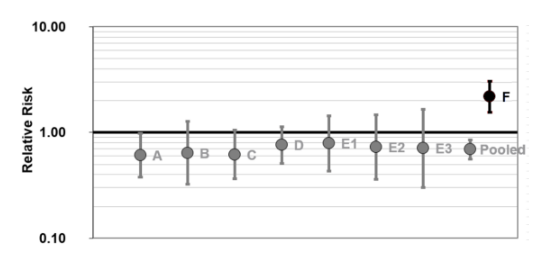
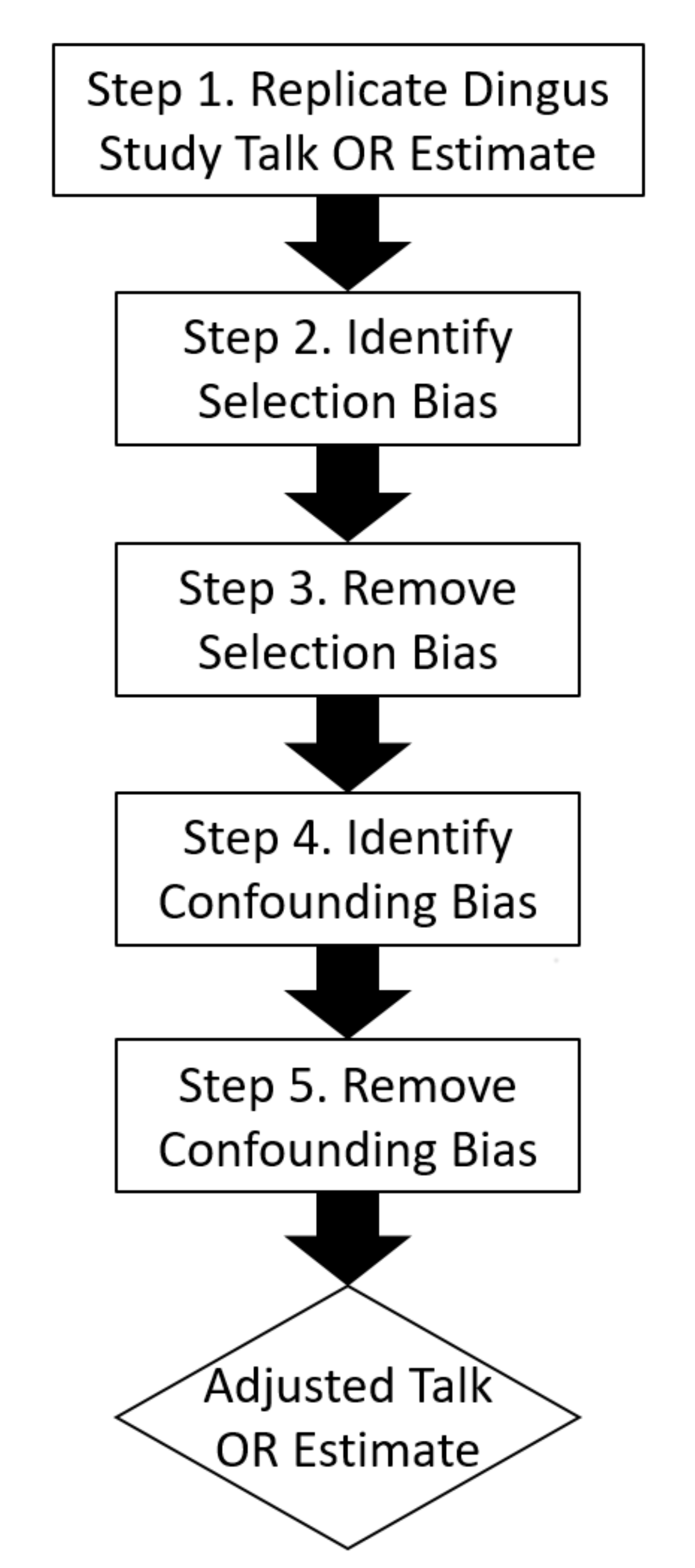
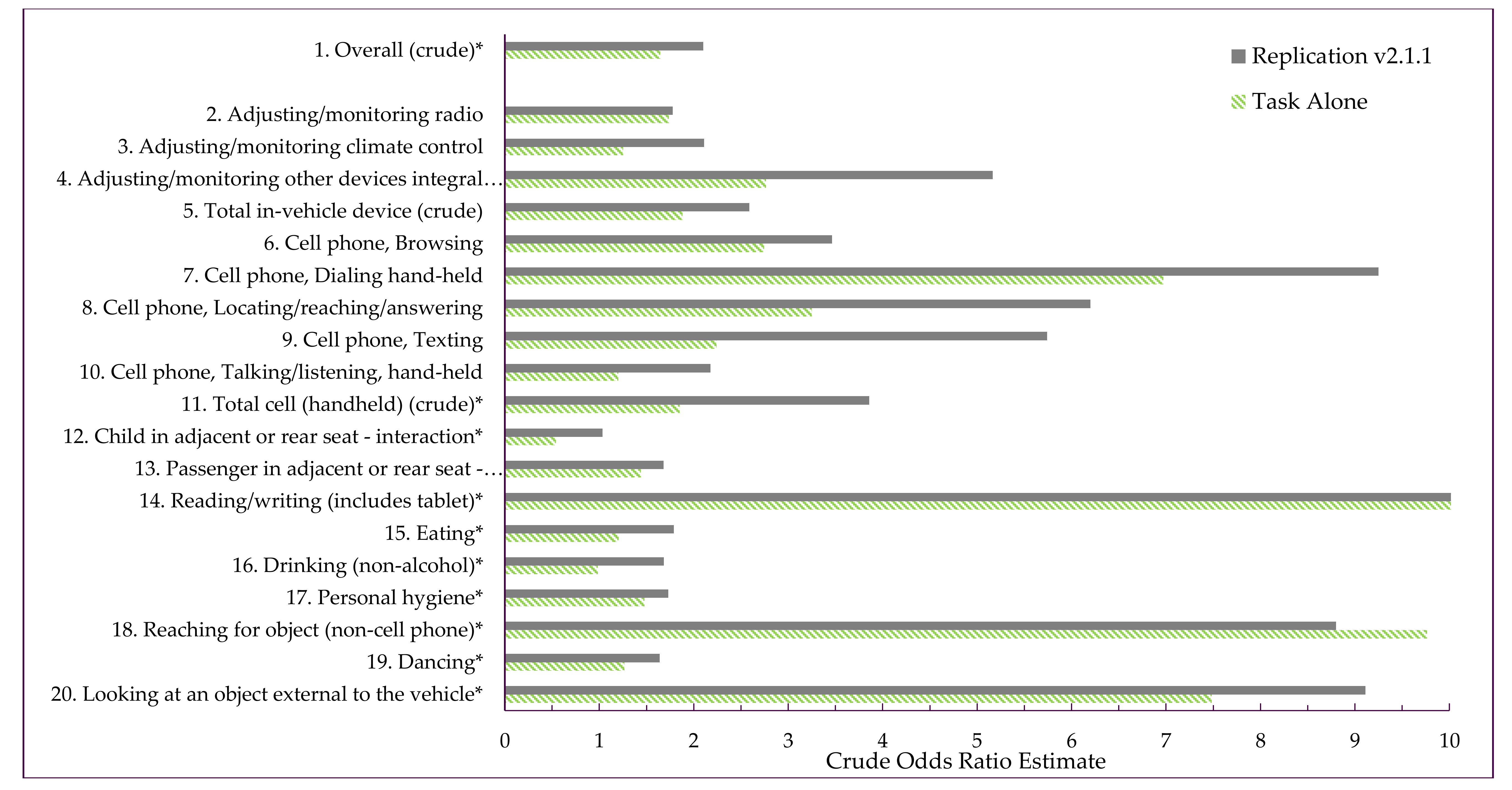
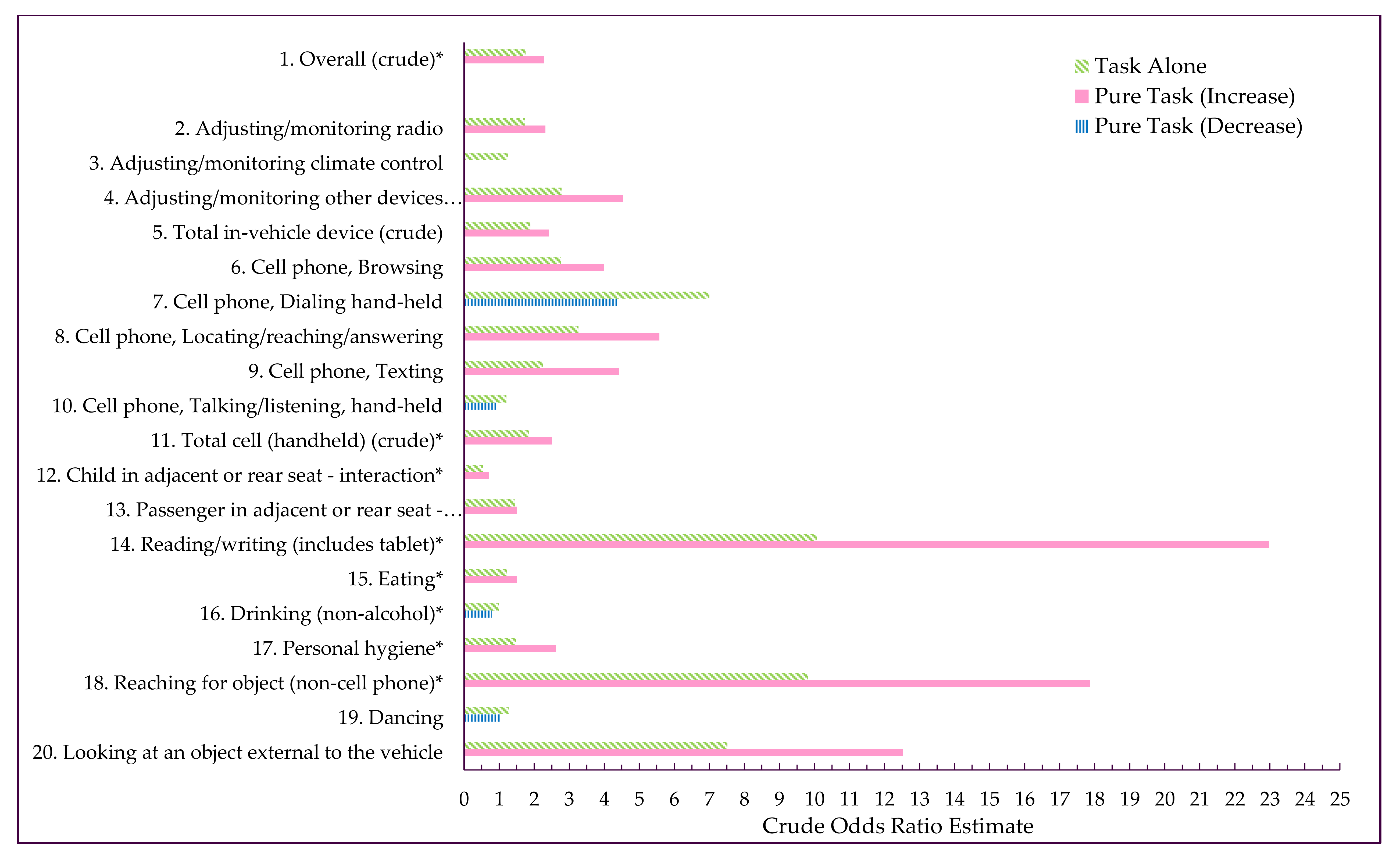
Table A1.
Studies of wireless cellular conversation (“Talk”) while driving a passenger vehicle.
| Study | Data | Event | Cases f | Location | Wireless Device | Study Design | Measure | Unexposed | Effect Size h | p |
|---|---|---|---|---|---|---|---|---|---|---|
| A. Redelmeier & Tibshirani (1997) [24] | real-world | I Severe b | 699 | Toronto | hand-held | case-crossover | adjusted rate ratio | Not Talk k | 0.61 (0.38–0.98) i | 0.03 |
| B. McEvoy et al. (2005) [25] | real-world | I Severe c | 456 | Australia | hand-held | case-crossover | adjusted rate ratio | Not Talk k | 0.64 (0.32–1.27) i | 0.20 |
| C. Young & Schreiner (2009) [37] | real-world | I Severe d | 2,037 | North America | integrated hands-free g | cohort | crude rate ratio | Not Talk k | 0.62 (0.37–1.05) | 0.07 |
| D. Klauer et al. (2014) [38] | 100-Car NDS j | I–IV & Near-Crash | 281 | Virginia | hand-held | case-control | adjusted OR | Not Talk k | 0.74 (0.51–1.06) | 0.10 |
| E1. Fitch et al. (2013) [16] | NDS j | SCE e | 13 | Virginia | hand-held | matched case-control | crude OR | No Task l | 0.79 (0.43–1.44) | 0.44 |
| E2. Fitch et al. (2013) [16] | NDS j | SCE e | 9 | Virginia | portable hands-free | matched case-control | crude OR | No Task l | 0.73 (0.36–1.47) | 0.37 |
| E3. Fitch et al. (2013) [16] | NDS j | SCE e | 6 | Virginia | integrated hands-free g | matched case-control | crude OR | No Task l | 0.71 (0.30–1.66) | 0.42 |
| Pooled A–E3 a | All | All | 3,803 | All | All | All | All | All | 0.69 (0.56–0.85) | 0.0005 |
| F. Dingus et al. (2016) [1] | SHRP 2 NDS j | I–III | 274 | U.S. | hand-held | case-control | crude OR | No Task l | 2.2 (1.6–3.1) | 0.000004 |
Notes: a p-value for homogeneity = 0.99. b Substantial property damage but no personal injury. c Injury requiring hospital attendance. d Airbag-deployment crash. e SCE = Safety Critical Event = Crash severities I–IV, Near-Crash and Crash-Relevant Conflict. f Number of cases used to estimate effect size. g Integrated non-portable hands-free wireless cellular device embedded into vehicle. h Effect size with lower and upper 95% confidence limits. i Adjusted rate ratio estimate from Young (2013b) [39]. j NDS = naturalistic driving study. k Not Talk = records can include secondary tasks other than Talk, as well as driver behavior errors and impairments. l No Task = records contain no secondary tasks but can include driver behavior errors and impairments.
Table A1 shows that prior epidemiological studies of Talk used a variety of epidemiological designs, from case-crossover (A,B), cohort (C), case-control (D), to matched case-control (E1–E3). Different study designs should give approximately the same effect size, if the studies are free of bias (Rothman, 2012) [10] (Chapter 5). The studies in Table A1 used widely different event levels, number of cases, geographic locations, wireless device types, study designs, effect size measures and unexposed type: Not Talk or No Task. It is therefore remarkable that all seven effect size estimates A–E3 in Table A1 were homogeneous with p = 0.99 (note a). This homogeneity indicates that Talk has the same effect size regardless of these varying parameters and so the effect measures can be validly pooled. The pooled OR estimate is 0.69 (CI 0.56–0.85), with a p-value of 0.0005, indicating that the upper limit of the 95% confidence interval is below 1 with high probability.
Appendix A.3. Discrepancy of Dingus Study Talk OR Estimate with Prior Studies
Figure A1.
Plot of effect size estimates in Table A1.
Figure A1.
Plot of effect size estimates in Table A1.

It is obvious by visual inspection of Figure A1, that the Dingus study Talk OR estimate (F) is an outlier compared to the 7 prior real-world and naturalistic driving study estimates (A–E3). Point F is not only substantially higher than the prior effect size estimates (A–E3) but also its point estimate is in the opposite direction from prior studies; i.e., above 1 rather than below 1. This visual impression is confirmed by a homogeneity test, which indicates that the Dingus Talk OR estimate (Point F) is strongly heterogeneous with the pooled Talk effect size of studies (A–E3) with p < 0.00000001.
As mentioned, these prior studies had a wide variety of epidemiological study designs, geographic locales, participants, wireless device types, etc. Hence, the substantial upward discrepancy of the Dingus study Talk OR estimate likely has little to do with any differences in any of these factors with the SHRP 2 dataset. Therefore, it was hypothesized before this study began that the Dingus study had one or more substantial upward biases that led to its high Talk OR point estimate compared to prior studies. The current study was therefore undertaken with the main objective of identifying those biases and adjusting or correcting for them to the extent possible.
Appendix A.4. Biases in Prior Studies A–E3
The prior studies A–E3 are next briefly reviewed, because later research has found that studies A and B (for example) were shown to have major biases and the effect sizes originally published in those studies had to be adjusted to correct for those biases. The corrected effect sizes are those shown in Table A1 and Figure A1.
Appendix A.4.1. Biases in Analyses of Case-Crossover Studies A and B
The case-crossover studies A and B originally had uncorrected risk ratio estimates above 6. Redelmeier and Tibshirani (1997) [24] and McEvoy et al. [25] correctly recognized that if a driver did not drive at all during the control window (what they termed driving intermittency), the risk ratio would be biased. To correct this bias, drivers who had an injury crash were asked to recall in a survey at a considerable time after the crash whether they drove in the control window the day before the crash which had the same ten-minute clock time (i.e., the time of the day or night) as the ten-minute case window before the crash. The investigators discarded these drivers from their analysis who did not recall driving during the control window time. They then adjusted the crude risk ratio estimates downwards to adjust for this confounding bias, from above six to near four.
The case-crossover authors were correct to adjust for total non-driving in control windows. Non-driving is a confounding bias for Talk, because non-driving is a common cause of both Talk exposure and the crash outcome. People reduce their Talk exposure when not driving, because the call rate is about 7 times lower when not driving (Young, 2013b) [39] (Section 2.2.3). It is obvious that the crash outcome is also greatly reduced when the vehicle ignition is off, because other drivers rarely crash into a parked vehicle. See Young (2011, 2012a, 2013b, 2014a) [35,39,40,41] and Young and Seaman (2012) [42] for details.
However, the case-crossover investigators falsely assumed that those drivers who did recall driving in the 10-min control window, actually drove during the entire ten-minute window. GPS studies (Young, 2011, 2012a; Young and Seaman, 2012) [40,41,42] find that driving times are highly variable from day-to-day and on average drivers who drive 10 min on one day, drive for only 2 min (20% of the time) on other days during the identical 10-min clock time. Young (2011,2012a) [40,41] was the first to recognize this additional driving bias in the case-crossover studies, which he termed part-time driving bias. In short, the case-crossover authors recognized and adjusted for “driving intermittency” (no driving in a control window) but they neither recognized nor adjusted for part-time driving in control windows. That is, they failed to adjust for the fact that Talk and crashes were being falsely counted when the vehicle ignition was off during an estimated 80% of the control window duration. Thus, the part-time driving in control windows gave rise to an additional substantial upward bias in the Talk RR. When the part-time driving bias effect was removed in the adjustment procedure, the case-crossover Talk risk ratio decreased from 4 to near 1. Part-time driving bias thus (falsely) elevated the case-crossover risk ratio estimates by about 4 times. After adjustment for both part-time driving bias and misclassification of calls as before the crash when they were after the crash, the Talk risk ratio point estimates from the case-crossover studies fell even further, from about 4 to 0.61 and 0.64 in studies A and B respectively—see Young (2013b) [39] for details. Questions were raised about these adjustments (Mittleman et al., 2012; McEvoy et al., 2012; Kidd and McCartt, 2012) [43,44,45] but they have been answered (Young, 2012b,c) [46,47].
Appendix A.4.2. Bias in OnStar Study C
Two real-world driving studies have been done using the OnStar wireless device. Studies using the OnStar wireless device rely upon GPS, crash sensors and wireless phone records to determine the exact times and locations of all crashes severe enough to deploy an airbag, along with all communications using an embedded wireless device (OnStar).
The first real-world study to call into question whether Talk had a high absolute risk was that of Young (2001) [48]. However, this large cohort study of 8 million OnStar advisor calls and airbag deployments could only collect data on Talk exposure and did not have a measure of non-exposure, so the study could not calculate a risk ratio or rate ratio.
Young and Schreiner (2009) [37] used OnStar personal calling and were able to establish a non-exposed baseline. They found a crude rate ratio of 0.62 (CI 0.37–1.05), in a large cohort study based on the timing information for 93 million conversations and 2037 Severity I airbag-deployment crashes in 3 million drivers. This study had 47,609 driving-years, more than an order of magnitude larger than SHRP 2 (Young, 2013b) [39] (footnote 10).
Fitch et al. (2013) [16] also did a cohort analysis of Talk in an integrated hands-free device (in addition to the case-control analysis shown in study E3 in Table A1) and found a rate ratio of 0.61 (CI 0.27–1.41) for summed crash severities I–IV, near-crashes and crash-relevant conflicts. This rate ratio for integrated hands-free devices confirms Young and Schreiner’s (2009) [37] rate ratio of 0.62 (CI 0.37–1.05), even though the latter is based solely on Severity I crashes that deployed an airbag. This highly consistent result suggests that the Talk effect size is homogeneous across the full range of safety-relevant events.
Young and Schreiner (2009) [37] noted a major limitation in their OnStar study, that they “did not have demographic information for individual users” at the time of their study. Therefore, their rate ratio of 0.62 reflects the aggregate OnStar cohort and has not been adjusted for age, sex, or other demographic variables. It is possible that the Talk crash rate ratio differed within demographic subgroups of the aggregate cohort. The Fitch et al. (2013) [16] and Dingus study OR estimates have the same limitation. However, as noted in Section A.6, analysis of the Klauer et al. (2014) [38] data found a homogeneous OR estimate for Talk between novice and experienced drivers. This result suggests that age (which is strongly correlated with driving experience) might not have substantially biased the Young and Schreiner (2009) [37] rate ratio of 0.62.
Another limitation noted by Braver et al. (2009) [49] was that the OnStar Talk rate ratio of 0.62 in the Young and Schreiner study may have been biased low because drivers might have been using hand-held cell phones in the OnStar-unexposed driving periods. If hand-held cell phones had 4.0 risk ratios such as that found in the case-crossover studies (Appendix A.4.1), then hand-held use in the OnStar-unexposed driving periods could have biased the OnStar rate ratio artificially low. However, later evidence does not support the Braver et al. claim for several reasons. First, Fitch et al. (2013) [16] found that drivers who used one type of cellular device (portable hands-free, portable hand-held, or embedded hands-free) rarely used another. Second, Fitch et al. (2013) [16] found that the OR estimates of all three types of cellular devices were about the same, with point estimates all below one (Table A1, points E1-E3). Third, the current study shows in the SHRP 2 data that the Talk OR estimates are homogeneous with point estimates both below 1 whether other tasks are present in the Talk-unexposed column (Table 6), or are not present in the Talk-unexposed column (Table 5).
Appendix A.4.3. Biases in Analysis of 100-Car Study D
In the original 100-Car NDS study, Klauer et al. (2006) [23] overestimated secondary task ORs because of several epidemiological biases—see Young (2013a,b; 2014a; 2015) [21,33,35,39]. For example, for safety-critical events (i.e., cases), Klauer et al. (2006) [23] chose all drivers (whether they were judged by the video reductionist as at-fault or not) for the Exposed column but chose only at-fault drivers (as judged by the video reductionist) for the Unexposed column. Eliminating this selection bias and other biases reduced the Klauer et al. (2006) [23] Talk OR estimate from 1.29 (CI 0.93–1.8) to 0.78 (CI 0.56–1.1) (Young, 2013a,b; 2014a) [33,35,39].
Klauer et al. (2014) [38] later also re-analyzed the 100-Car dataset and eliminated these biases. They found a Talk OR estimate of 0.61 (CI 0.24–1.57) for novice drivers and 0.76 (CI 0.51–1.13) for experienced drivers. These two OR estimates are homogeneous (p = 0.67) so they were here combined into a pooled estimate of 0.74 (CI 0.51–1.06), with p-value = 0.099 (see study D in Appendix A, Table A1). This Klauer et al. pooled 100-Car Talk OR estimate of 0.74 validates the prior adjusted 100-Car Talk OR estimate of 0.78 (CI 0.56–1.1) made by Young (2013a,b; 2014a) [33,35,39]. The Dingus study [1] avoided the biases in the Klauer et al. (2006) [23] study identified by Young (2013a,b; 2014a; 2015) [21,33,35,39], but the current study presents evidence that the Dingus study introduced new upward biases in its secondary task OR estimates.
Appendix A.4.4. Biases in Cell Phone Study E
The Fitch et al. (2013) [16] cell phone study tabulated demographic and environmental variables in its Appendices, did not adjust its rate ratios and OR estimates for those variables. Hence its crude rate ratio and OR estimates may be biased either high or low from their true values. It did however use baseline control windows shortly before the time of the case windows, creating a matched case-control design and minimizing the biasing effect of demographic and environmental variables.
Appendix A.5. Homogeneity and Pooling of Prior Studies
In summary, after adjustment of the risk ratios in studies A and B, the effect size estimates of Talk in the real-world and naturalistic studies A to E3 in Table A1 and Figure A1 are homogeneous (p = 0.99). Homogeneity means that they provide a common population estimate of the Talk risk ratio, despite differences in crash severity level, location, type of wireless device (hand-held, hands-free, or embedded hands-free), study design, or the unexposed condition (No Talk or No Task). Because of this homogeneity, the estimates could be validly pooled in a meta-analysis using Episheet (Rothman, 2015) [30]. The pooled OR estimate of 0.69 (CI 0.56–0.85) indicates a net protective effect during Talk; that is, crashes are reduced during Talk.
One plausible explanation is driver self-regulation (Young, 2014b) [20], which can give rise to displacements (i.e., reductions) (Victor et al., 2015) [50] of driver activities or driver states that may increase risk. Some of the known driver activity reductions during Talk are: reductions in driver behavior errors such as speeding (Young, 2017b) [14]; reductions in multi-tasking with additional secondary tasks (Young, 2014b) [20]; and temporary reductions in drowsiness (Young, 2013c) [29].
Appendix B. Formal Definition and Evidence for Confounding Bias
Appendix B.1. Formal Definition of Confounding Bias
A formal epidemiological definition of confounding bias is given by Porta (2014) [11] (p. 55), “Bias of the estimated effect of an exposure on the outcome due to the presence of common causes of the exposure and the outcome”. In other words, confounding bias occurs when all or part of the apparent association between the exposure and outcome is in fact accounted for by other variables that affect the outcome and are not themselves affected by the exposure. The SHRP 2 data examined in Section 3.3 indicate that a substantial proportion of SHRP 2 drivers engaged in driver behavior errors at the same time as they engaged in secondary tasks.
Appendix B.2. Proof of Confounding Bias from Driver Behavior Errors
To meet the formal epidemiological definition of confounding in the above Section B.1, driver behavior errors must affect both crashes and secondary task exposure. In other words, the two requirements for confounding are: (1) Driver behavior errors must affect the event outcome (a crash); and (2) Driver behavior errors must affect the secondary task exposure (in this example, Talk). The following subsections show that driver behavior errors meet both requirements and are therefore a confounding factor for the Talk OR estimate.
Appendix B.2.1. Confounding Requirement 1: Driver Behavior Errors Affect Crash Odds
Confounding requirement 1 is met because driver behavior errors are well established to substantially increase the odds of a crash. Some examples are:
- In the Dingus study, before adjustment for biases, “Right-of-way” error had a crude OR estimate of 936 (CI 124–7078) and “Sudden or improper braking/stopping” error had a crude OR estimate of 248 (CI 53.1–1,156).
- After adjustment for biases, the adjusted OR estimate for “Exceeded speed limit” in the SHRP 2 database was 5.4 (CI 2.7–10.1) and for “Exceeded safe speed but not speed limit” was 72 (CI 37–136) (Young, 2017b) [14].
- Table 1 in the main body of this paper reveals that crashes have a substantially elevated proportion of driver behavior errors, compared to baselines, in the absence of secondary tasks (the Unexposed column, or “Model Driving”). Indeed, 141 (60%) of the 235 Talk-unexposed crash cases had driver behavior errors (note x) but only 1538 (8.3%) of the Talk-unexposed 9420 baseline controls did (note z). A difference of proportions test in Stata [3] finds an extraordinarily high Z value of 26.6, with p near 0, so crashes definitely have a higher proportion of driver behavior errors than baselines.
The SHRP 2 video reduction methods (VTTI, 2015) [8] do not state that the video reductionists are “blinded” as to whether there was a crash or not in the video record they are analyzing. If they are not “blinded,” it is plausible that they scrutinize crash records more carefully for driver behavior errors than they do baseline records. For example, crash videos might be more carefully examined than baseline videos for stop/yield sign and traffic signal violations. However, “Exceeded speed limit,” with the largest baseline prevalence at 2.77%, is an objective measurement from GPS or the vehicle speedometer instrumentation and does not require video clip observations. In sum, it is plausible that drivers making behavior errors have a higher odds of crashing than drivers who do not, meeting confounding requirement 1.
Appendix B.2.2. Confounding Requirement 2: Driver Behavior Errors Affect Talk Exposure
Confounding requirement 2 is met if drivers making a behavior error alter their Talk exposure during that behavior. To determine if that is true, the proportion of Talk exposure with and without driver behavior errors may be compared, with additional tasks held constant. Table 2 in the main body shows that with no additional tasks, Talk0b had 47 (8.8%) of 534 exposed baseline records with driver behavior errors (note y). During Not Talk0b, 141 (60%) of the 235 Talk-unexposed crash cases had driver behavior errors (note x, same as Table 1). A difference of proportions test in Stata [3] between the proportion of behavior errors during Talk vs. Not Talk finds a Z value of 5.07, with p = 0.0000004. That is, baseline records with Talk exposure have a substantially lower proportion of driver behavior errors than baseline records without Task exposure. In other words, during Talk while baseline driving, drivers make fewer driver behavior errors than during Not Talk. The converse is that when a baseline record shows a driver is making a driver behavior error, the probability of Talk is reduced. In short, driver behaviors errors alter Talk exposure, meeting confounding requirement 2.
Appendix B.2.3. Empirical Proof that Driver Behavior Errors Confound the Talk OR Estimate
A second method to prove the confounding is from the direct empirical evidence of the effect of removing the bias. When driver behavior errors are removed from the Talk OR estimate by simply filtering out all driver behavior errors, leaving everything else constant, the Talkab OR estimate declines from 1.4 (CI 0.95–2.0) in Table 4, to the Talka0 OR estimate of 0.92 (CI 0.45–1.7) in Table 6. Hence, confounding from driver behavior errors increased the OR point estimate from 0.92 to 1.4. Similarly, the Talk0b OR estimate declines from 1.2 (CI 0.67–2.0) in Table 2, to the Talk00 OR estimate of 0.94 (CI 0.30–2.3) in Table 6. Hence, confounding from driver behavior errors must have increased the OR point estimate in both comparisons.
Appendix B.3. Consequences of Confounding Bias from Driver Behavior Errors
Note that “driver behavior errors” are present not just in Table 1 but also in Table 2, Table 3 and Table 4. Therefore, confounding bias from driver behavior errors is present in all the Table 1, Table 2, Table 3 and Table 4 presented in the main body of the current paper. That is, all OR estimates in Table 1, Table 2, Table 3 and Table 4 in this paper may not be valid estimates of the Talk OR estimate when combined with other secondary tasks (Table 1, Table 3 and Table 4), or not (Talk Alone, Table 2). All these Talk OR estimates are likely confounded by “driver behavior errors,” which can bias the Talk OR estimates.
Hence, the Dingus study Talk OR estimate of 2.2 (CI 1.5–3.1) in Table 1 (main body of current article) reflects not just the OR estimate of Talk with additional secondary tasks but also the confounding effect of driver behavior errors. Likewise, the Talk OR estimate of 1.2 (CI 0.67–2.0) in Table 2 (main body of current article) after removal of selection bias, still represents the effect of Talk confounded with driver behavior errors. In either scenario, the presence of driver behavior errors could thus bias secondary task OR estimates by additive, multiplicative, or supra-multiplicative confounding effects.
At a minimum, an additive effect would occur, because the OR estimates of driver behavior errors are substantially higher than the OR estimates for secondary tasks, as noted in Section B.2.1 A supra-multiplicative interaction effect that would substantially increase relative crash risk would also arise if the interactive effects of multi-tasking secondary tasks with one or more driver behavior errors (simultaneously or near-simultaneously with one or more secondary tasks) causes a biologic interaction effect (Rothman, 2012, p. 182) [10]. A theory for and evidence for this biologic interaction effect in driving safety, was first advanced for the SHRP 2 data by Young (2017a) [7] (Appendix B and Appendix C) and further evidence was provided by Young (2017b) [14]. These biologic interaction effects of driver behavior errors with secondary tasks are likely even greater than they are for interactions just between secondary tasks; see Section 4.1.4 and Young (2017a) [7] (Appendix B and Appendix C).
Appendix C. Secondary Task OR Estimates in Dingus Study vs. Current Replication
Table A2B shows the replication that most closely matches the Dingus study secondary task OR estimates in Table A2A.
Table A2.
(A) Dingus study secondary task OR estimates. (B) Current study replication.
| A. Original Dingus Study Results | B. Replication (SHRP 2 Database version 2.1.1) | |||||||||||||||
|---|---|---|---|---|---|---|---|---|---|---|---|---|---|---|---|---|
| Observable Distraction | OR | LL | UL | Base. Prev. | Observable Secondary Task or Task Category a | OR | LL b | UL b | Base. Prev. c | Pooled Tasks | Exposed Crashes | Exposed Baselines | pl | |||
| 1. Overall | 2.0 | 1.8 | 2.4 | 51.93% | Overall * | 2.1 | 1.8 | 2.5 | 51.98% | 43 | 540 | 10,197 | 0.63 | |||
| Major Categories: | Major Categories: | |||||||||||||||
| 2. In-vehicle radio | 1.9 | 1.2 | 3.0 | 2.21% | Adjusting/monitoring radio | 1.8 | 1.1 | 2.8 | 2.30% | 1 | 20 | 451 | 0.84 | |||
| 3. In-vehicle climate control | 2.3 | 1.1 | 5.0 | 0.56% | Adjusting/monitoring climate control | 2.1 | 0.8 | 4.8 | 0.58% | 1 | 6 | 114 | 0.88 | |||
| 4. In-vehicle device (other) | 4.6 | 2.9 | 7.4 | 0.83% | Adjusting/monitoring other devices integral to the vehicle | 5.2 | 3.1 | 8.3 | 0.83% | 1 | 21 | 163 | 0.74 | |||
| 5. Total in-vehicle device | 2.5 | 1.8 | 3.4 | 3.53% | Total in-vehicle device | 2.6 | 1.8 | 3.6 | 3.71% | 3 | 47 | 728 | 0.88 | |||
| 6. Cell browse | 2.7 | 1.5 | 5.1 | 0.73% | Cell phone, Browsing | 3.5 | 1.8 | 6.1 | 0.83% | 1 | 14 | 162 | 0.57 | |||
| 7. Cell dial (handheld) | 12.2 | 5.6 | 26.4 | 0.14% | Cell phone, Dialing hand-held † | 9.3 | 3.1 | 23.2 | 0.13% | 1 | 6 | 26 | 0.65 | |||
| 8. Cell reach | 4.8 | 2.7 | 8.4 | 0.58% | Cell phone, Locating/reaching/answering | 6.2 | 3.6 | 10.4 | 0.62% | 1 | 19 | 122 | 0.50 | |||
| 9. Cell text (handheld) | 6.1 | 4.5 | 8.2 | 1.91% | Cell phone, Texting | 5.7 | 4.1 | 7.9 | 1.96% | 1 | 55 | 384 | 0.78 | |||
| 10. Cell talk (handheld) | 2.2 | 1.6 | 3.1 | 3.24% | Cell phone, Talking/listening, hand-held | 2.2 | 1.5 | 3.2 | 3.19% | 1 | 34 | 626 | 0.97 | |||
| 11. Total cell (handheld) | 3.6 | 2.9 | 4.5 | 6.40% | Total cell (handheld) * | 3.9 | 3.1 | 4.9 | 6.73% | 5 | 128 | 1,320 | 0.64 | |||
| 12. Child rear seat | 0.5 | 0.1 | 1.9 | 0.80% | Child in adjacent/rear seat—interaction *,d | 1.0 | 0.3 | 2.5 | 0.99% | 2 d | 5 | 194 | 0.37 | |||
| 13. Interaction with adult or teen passenger | 1.4 | 1.1 | 1.8 | 14.58% | Passenger in adjacent or rear seat—interaction *,e | 1.7 | 1.3 | 2.1 | 15.20% | 2 e | 125 | 2,982 | 0.29 | |||
| 14. Reading/writing (includes tablet) | 9.9 | 3.6 | 26.9 | 0.09% | Reading/writing (includes tablet) *,f | 10.0 | 2.9 | 27.8 | 0.10% | 5 f | 5 | 20 | 0.99 | |||
| 15. Eating | 1.8 | 1.1 | 2.9 | 1.90% | Eating with/without utensils *,g | 1.8 | 1.0 | 3.0 | 1.94% | 2 g | 17 | 381 | 0.99 | |||
| 16. Drinking (non-alcohol) | 1.8 | 1.0 | 3.3 | 1.22% | Drinking (non-alcohol) *,h | 1.7 | 0.8 | 3.2 | 1.21% | 4 h | 10 | 238 | 0.88 | |||
| 17. Personal hygiene | 1.4 | 0.8 | 2.5 | 1.69% | Personal hygiene *,i | 1.7 | 1.1 | 2.5 | 3.78% | 9 i | 32 | 741 | 0.55 | |||
| 18. Reaching for object (non-cell phone) | 9.1 | 6.5 | 12.6 | 1.08% | Reaching for object (non-cell phone) *,j | 8.8 | 6.1 | 12.5 | 1.09% | 5 j | 47 | 213 | 0.91 | |||
| 19. Dancing in seat to music | 1.0 | 0.4 | 2.3 | 1.10% | Dancing | 1.6 | 0.7 | 3.2 | 1.12% | 1 | 9 | 220 | 0.37 | |||
| 20. Extended glance duration to ext. object | 7.1 | 4.8 | 10.4 | 0.93% | Looking at an object external to the vehicle k | 9.1 | 5.8 | 13.9 | 0.67% | 1 | 30 | 132 | 0.39 | |||
Notes: a Observable from 6-second pre-crash and baseline sample video segments. b Based on exact 95% confidence limit from Stata 13 epidemiology function “cci”. c Baseline prevalence is the baseline exposed count divided by the current study balanced-sample baseline record total of 19,617. d “Child in adjacent seat—interaction” + “Child in rear seat—interaction”. e “Passenger in adjacent seat - interaction” + “Passenger in rear seat—interaction”. f “Reading” + “Writing” + “Tablet device, Operating” + “Tablet device, Viewing” + “Tablet device, Other”. g “Eating with utensils” + “Eating without utensils”. h “Drinking with lid and straw” + “Drinking with lid, no straw” + “Drinking with straw, no lid” + “Drinking from open container”. i “Combing/brushing/fixing hair” + “Applying make-up” + “Shaving” + “Brushing/flossing teeth” + “Biting nails/cuticles” + “Removing/adjusting clothing” + “Removing/adjusting jewelry” + “Removing/inserting/ adjusting contact lenses or glasses”. j “Reaching for object, other” + “Tablet device, Locating/reaching” + “Reaching for food-related or drink-related item” + “Reaching for cigar/cigarette”“ + “Reaching for personal body-related item”. k There was no task in the database called “Extended glance duration to external object”. The closest fit was, “Looking at an object external to the vehicle”. l p-value for homogeneity between the Dingus study OR estimate and the current study replication. * Task categories formed in Dingus study by pooling tasks with heterogeneous OR estimates that should not be combined. † Task “7. Cell phone, dialing hand-held” typically had the following additional tasks present with it in the same SHRP 2 database record: “10. Cell phone, Talking/listening, hand-held” and “Cell phone, Holding”. In fact, there were no crash cases of dialing by itself; it was always accompanied in the 6-s case window with talking and/or holding the phone. Dialing by itself also rarely occurred during the 6-s baseline control window; holding or talking on the phone almost always accompanied it. Although the phones were all hand-held in the SHRP 2 study OR estimates, it is not stated in the narratives but conceivable that in some instances the driver may have had the phone mounted so they could manually dial without holding it.
Table A2A lists what the Dingus study terms “Observable Distractions” and their secondary task OR estimates in that study. The replication in Table A2B shows that all 20 replicated OR estimates were homogeneous with their corresponding original Dingus study OR estimate. That is, the p-value for homogeneity in the right-most column is always greater than the usual 0.05 criterion, meaning the hypothesis of homogeneity cannot be rejected.
Task Categories
Table A2B labels the “Observable Distractions” column in Table A2A with the more objective term “Observable Secondary Task or Task Category”.
It was discovered during the replication that most of the “Observable Distraction” names in the Dingus study (see Table A2A) are not actually present in the SHRP 2 database as single secondary tasks. The names not found in the database are “Observable Distraction” numbers 1, 5, 11, 12–18 and 20. The replication found that these were actually summations of secondary tasks that the Dingus study had formed by combining secondary tasks in the SHRP 2 database, not single secondary tasks. The Dingus study did not indicate which secondary tasks it had summed together to form these categories.
The replication therefore had to make the best estimate it could of the secondary tasks that were summed together by the Dingus study to form those categories, by finding those tasks whose sum gave the closest OR estimate to each of the 20 Dingus study “Observable Distractions”. The task categories in Table A2B are those in the SHRP 2 database version 2.1.1 that best matched the “Observable Distraction” names in the Dingus study as shown in Table A2A. The single tasks that were summed are indicated in notes d–j for Table A2B.
These task categories were checked for homogeneity between the summed tasks and almost all were heterogeneous (indicated with an asterisk at the end of the task names in Table A2B). Heterogeneity means that the task OR estimates should have been separately reported and not pooled together as was done by the Dingus study.
Note also that the replication found that “Overall” category 1 is not the sum of the categories 5, 11 and 12–20 as was expected from the layout of Table A2A. The balanced-sample baseline prevalence for “Overall Distraction” is given by the Dingus study as 51.93%. However, the sum of the baseline prevalence for the “Observable Distractions” in lines 5, 11 and 12–20 in Table A2A is only 33.32%. The replication in Table A2B found that all 10,197 exposed secondary task records for the 43 secondary tasks in the baseline database were apparently used in the Dingus study rather than the 39 “pooled tasks” in Table A3B. The replicated “Overall Secondary Task” prevalence of 51.98% is then consistent with the Dingus study “Overall” prevalence of 51.93% for “Observable Distractions”. It therefore appears that the Dingus study calculated its “Overall” prevalence estimate based on all secondary tasks in the SHRP 2 database version 1.0 that they used. The “Overall” OR replicated estimate in Table A2B for all secondary tasks is 2.1 (CI 1.8–2.5), which is homogeneous with the Dingus Study “Overall” estimate of 2.0 (CI 1.8–2.4) with probability 0.71, which shows the replication of the Dingus study “Overall” OR estimate was successful. Note however that the replication found that secondary task categories 1 and 11–18 were formed from secondary tasks with heterogeneous OR estimates and therefore should not have been pooled by the Dingus study.
Note that Appendix Table A2B in the current article is based on version 2.1.1 of the SHRP 2 database; a similar Appendix Table A3B in Young (2017a) [7] is based on the earlier version 2.0.0 of the SHRP 2 database. There are some slight reductions in the crash counts and the baseline counts in the two versions, because several crash and baseline records were dropped in version 2.1.1 according to the release notes. These are the likely cause of the slight differences in the OR estimates and confidence limits in the Appendix Table A2B in the current article and the Appendix Table A3B in Young (2017a) [7].
Appendix D. Dingus Study Replication with Biases Removed
Appendix D gives the OR estimates for the Dingus study secondary task categories with biases removed as per the procedure in Table 1 in the main body. Table A3A removes selection bias in the Table A2B replication. Table A3B then removes the driver behavior error confounding bias from Table A3A.
Table A3.
(A) OR estimates after removing selection bias. (B) OR estimates after removing selection and confounding bias.
Table A3.
(A) OR estimates after removing selection bias. (B) OR estimates after removing selection and confounding bias.
| A. Secondary Tasks Alone vs. “Model Driving” (Selection Bias Removed) | B. Pure Tasks vs. Pure Baseline Driving (Both Biases Removed) | ||||||||||||
|---|---|---|---|---|---|---|---|---|---|---|---|---|---|
| Observable Secondary Task or Task Category a | OR | LL b | UL b | Baseline Prev.c | Exposed Crashes | Exposed Baselines | OR | LL b | UL b | Baseline Prev. c | Exposed Crashes | Exposed Baselines | |
| 1. Overall * | 1.6 | 1.4 | 2.0 | 41.08% | 331 | 8058 | 2.1 | 1.6 | 2.7 | 37.87% | 168 | 7428 | |
| Major Categories: | |||||||||||||
| 2. Adjusting/monitoring radio | 1.7 | 0.4 | 2.3 | 1.29% | 11 | 254 | 2.3 | 0.8 | 5.3 | 1.21% | 6 | 238 | |
| 3. Adjusting/monitoring climate control | 1.3 | 0.1 | 4.8 | 0.33% | 2 | 64 | 0.0 | 0.0 | 5.9 | 0.31% | 0 | 60 | |
| 4. Adjusting/monitoring other devices integral to vehicle | 2.8 | 0.5 | 5.3 | 0.44% | 6 | 87 | 4.5 | 1.2 | 12.5 | 0.41% | 4 | 81 | |
| 5. Total in-vehicle device | 1.9 | 0.5 | 2.0 | 2.06% | 19 | 405 | 2.4 | 1.1 | 4.7 | 1.93% | 10 | 379 | |
| 6. Cell phone, Browsing | 2.7 | 1.1 | 3.0 | 0.37% | 5 | 73 | 4.0 | 0.8 | 12.5 | 0.35% | 3 | 69 | |
| 7. Cell phone, Dialing hand-held † | 7.0 | 1.7 | 20.6 | 0.12% | 4 | 23 | 4.4 | 0.1 | 27.8 | 0.11% | 1 | 21 | |
| 8. Cell phone, Locating/reaching/answering | 3.3 | 0.6 | 10.4 | 0.19% | 3 | 37 | 5.6 | 0.6 | 22.3 | 0.17% | 2 | 33 | |
| 9. Cell phone, Texting | 2.2 | 1.7 | 20.6 | 1.46% | 16 | 286 | 4.4 | 2.2 | 8.1 | 1.38% | 13 | 270 | |
| 10. Cell phone, Talking/listening, hand-held | 1.2 | 0.7 | 2.0 | 2.72% | 16 | 534 | 0.9 | 0.3 | 2.3 | 2.48% | 5 | 487 | |
| 11. Total cell (handheld) * | 1.9 | 1.3 | 2.6 | 4.86% | 44 | 953 | 2.5 | 1.5 | 4.0 | 4.49% | 24 | 880 | |
| 12. Child in adjacent/rear seat—interaction *,d | 0.5 | 0.1 | 2.0 | 0.75% | 2 | 148 | 0.7 | .02 | 4.1 | 0.66% | 1 | 130 | |
| 13. Passenger in adjacent or rear seat—interaction *,e | 1.4 | 1.1 | 1.9 | 11.5% | 81 | 2253 | 1.5 | 1.0 | 2.2 | 10.6% | 34 | 2089 | |
| 14. Reading/writing (includes tablet) *,f | 10.0 | 0.2 | 101.7 | 0.02% | 1 | 4 | 23.0 | 0.5 | 234.6 | 0.02% | 1 | 4 | |
| 15. Eating with/without utensils *,g | 1.2 | 0.5 | 2.4 | 1.36% | 8 | 266 | 1.5 | 0.4 | 4.0 | 1.25% | 4 | 245 | |
| 16. Drinking (non-alcohol) *,h | 1.0 | 0.2 | 3.0 | 0.62% | 3 | 122 | 0.8 | .02 | 4.6 | 0.59% | 1 | 116 | |
| 17. Personal hygiene *,i | 1.5 | 0.8 | 2.4 | 2.35% | 17 | 461 | 2.6 | 1.3 | 4.8 | 2.15% | 12 | 422 | |
| 18. Reaching for object (non-cell phone) *,j | 9.8 | 5.5 | 16.6 | 0.40% | 19 | 78 | 17.9 | 9.0 | 33.4 | 0.37% | 14 | 72 | |
| 19. Dancing | 1.3 | 0.3 | 3.9 | 0.48% | 3 | 95 | 1.0 | 0.0 | 6.1 | 0.45% | 1 | 88 | |
| 20. Looking at an object external to the vehicle k | 7.5 | 3.8 | 13.6 | 0.38% | 14 | 75 | 12.5 | 5.3 | 26.2 | 0.34% | 9 | 66 | |
Notes: a–k Same as Table A2. † Dialing was the only task or task category allowed to have certain additional tasks present for “Task Alone” or “Pure Task”. See corresponding note in Table A2 for additional tasks that were typically present with dialing. * Task categories incorrectly formed by Dingus study by pooling tasks with heterogeneous OR estimates.
Figure A2 compares the replicated Dingus study secondary task OR point estimates from Appendix B Table A2B (solid gray bars), vs. the OR point estimates for “Task Alone” from Appendix D Table A3A (diagonally-hatched green bars), with the selection bias removed. (Task Alone means the secondary task category by itself with no additional secondary tasks in the database records.) The “Task Alone” bars are the last two columns in Table A2B. Figure A2 shows that the OR point estimate for every “Task Alone” category except for “18. Reaching for object (non-cell phone)” declines after the additional task selection bias is removed, as expected from the Talk task example in Table 2 in the main body of this paper. The Talk task from Table 2 in the main body is shown as Task 10 in Figure A2 (see the bar values for Task 10 in Table A2B and Table A3A).
Figure A2.
Solid gray bars: Replicated Dingus study secondary task category OR point estimates from Appendix B Table A2B. Diagonally-hatched green bars: Current “Task Alone” OR point estimates from Appendix D Table A3A. * indicates the category was formed from heterogeneous tasks that should not have been combined.

Figure A3 replots the “Task Alone” OR point estimates in Figure A2 (diagonally-hatched green bars). These are now compared to the “Pure Task” point estimates from Table A3B which also removes driver behavior error confounding bias. The “Pure Tasks” with decreased OR point estimates after removal of driver behavior error confounding bias are the vertically-hatched blue bars (task categories 7, 10, 16 and 19). The “Pure Tasks” with increased OR point estimates after that removal are the solid red bars (all other tasks or task categories).
Figure A3.
Task Alone compared to Pure Task. Diagonally-hatched green bars: “Task Alone” OR point estimates (same as hatched bars in Figure A2). Vertically-hatched blue bars: “Pure Tasks” with decreased OR point estimates after driver behavior errors removed. Solid red bars: “Pure Tasks” with increased OR point estimates after driver behavior errors removed. * indicates the category was formed from heterogeneous tasks that should not have been combined.

References
- Dingus, T.A.; Guo, F.; Lee, S.; Antin, J.F.; Perez, M.; Buchanan-King, M.; Hankey, J. Driver crash risk factors and prevalence evaluation using naturalistic driving data. Proc. Natl. Acad. Sci. USA 2016, 113, 2636–2641. Available online: https://www.researchgate.net/profile/Jonathan_Antin/publication/ (accessed on 30 May 201). [CrossRef] [PubMed]
- Dingus, T.A.; Guo, F.; Lee, S.; Antin, J.F.; Perez, M.A.; Buchanan-King, M.; Hankey, J. Driver Crash Risk Factors and Prevalence Evaluation using Naturalistic Driving Data. VTTI Root Dataverse, V1; In Transportation Research Board of the National Academies; Virginia Tech Transportation Institute: Blacksburg, VA, USA, 2016. [Google Scholar]
- ‘Stata 13.’. Available online: https://www.stata.com/ (accessed on 11 October 2016).
- Greenland, S.; Senn, S.J.; Rothman, K.J.; Carlin, J.B.; Poole, C.; Goodman, S.N.; Altman, D.G. Statistical tests, p values, confidence intervals and power: A guide to misinterpretations. Eur. J. Epidemiol. 2016, 31, 337–350. Available online: https://link.springer.com/article/10.1007%2Fs10654-016-0149-3 (accessed on 11 October 2016). [CrossRef] [PubMed]
- Rothman, K.J. Disengaging from statistical significance. Eur. J. Epidemiol. 2016, 31, 443–444. Available online: http://link.springer.com/article/10.1007%2Fs10654-016-0158-2 (accessed on 30 May 2017). [CrossRef] [PubMed]
- Transportation Research Board of the National Academy of Sciences. The 2nd Strategic Highway Research Program Naturalistic Driving Study InSight Dataset (Version 2.1.1). 2016. Available online: https://insight.shrp2nds.us (accessed on 30 May 2017).
- Young, R.A. Removing Biases from Crash Odds Ratio Estimates of Secondary Tasks: A New Analysis of the SHRP 2 Naturalistic Driving Study Data; SAE Technical Paper 2017-01-1380.01 (revised); 2017. Available online: https://www.researchgate.net/publication/319690973 (accessed on 28 November 2017).
- VTTI (Virginia Tech Transportation Institute). Researcher Dictionary for Safety Critical Event Video Reduction Data. 2015. Available online: https://vtechworks.lib.vt.edu/bitstream/handle/10919/56719/V4.1_ResearcherDictionary_for_VideoReductionData_COMPLETE_Oct2015_10–5-15.pdf?sequence=1&isAllowed=y (accessed on 30 May 2017).
- Ahlstrom, C.; Fors, C.; Anund, A.; Hallvig, D. Video-based observer rated sleepiness versus self-reported subjective sleepiness in real road driving. Eur. Transp. Res. Rev. 2015, 7, 38. [Google Scholar] [CrossRef]
- Rothman, K.J. Epidemiology: An Introduction, 2nd ed.; Oxford University Press: New York, NY, USA, 2012; ISBN 978-0-19-975455-7. [Google Scholar]
- Porta, M. A Dictionary of Epidemiology., 6th ed.; Oxford University Press: New York, NY, USA, 2014; ISBN1 0199390053. Available online: http://irea.ir/files/site1/pages/dictionary.pdf (accessed on 16 October 2017)ISBN2 0199390053.
- Posner, M.I.; Fan, J. Attention as an organ system. In Topics in Integrative Neuroscience: From Cells to Cognition; Pomerantz, J.R., Ed.; Cambridge University Press: Cambridge, UK, 2008; pp. 31–61. [Google Scholar]
- Foley, J.; Young, R.; Angell, L.; Domeyer, J. Towards Operationalizing Driver Distraction. In Proceedings of the 7th International Driving Symposium on Human Factors in Driver Assessment, Training and Vehicle Design, Bolton Landing, NY, USA, 17–20 June 2013; Available online: https://www.researchgate.net/profile/Richard_Young9/publication/259908595 (accessed on 30 May 2017).
- Young, R.A. Adjusted Crash Odds Ratio Estimates of Driver Behavior Errors: A Re-Analysis of the SHRP 2 Naturalistic Driving Study Data. Proceedings of Driving Assessment 2017: The 9th International Driving Symposium on Human Factors in Driver Assessment, Training and Vehicle Design, Manchester Village, VT, USA, 26−29 June 2017. [Google Scholar]
- Green, P.; George, J.; Jacob, R. What Constitutes a Typical Cell Phone Call? UMTRI 2003-38; University of Michigan Transportation Research Institute: Ann Arbor, MI, USA, 2004; Available online: https://deepblue.lib.umich.edu/bitstream/handle/2027.42/92351/102883.pdf?sequence=1&isAllowed=y (accessed on 30 May 2017).
- Fitch, G.M.; Soccolich, S.A.; Guo, F.; McClafferty, J.; Fang, Y.; Olson, R.L.; Perez, M.A.; Hanowski, R.J.; Hankey, J.M.; Dingus, T.A. The Impact of Hand-Held and Hands-Free Cell Phone Use on Driving Performance and Safety-Critical Event Risk Final Report; NHTSA: Washington, DC, USA, 2013; Available online: http://www.nhtsa.gov/DOT/NHTSA/NVS/Crash%20Avoidance/Technical%20Publications/2013/811757.pdf (accessed on 30 May 2017).
- Bhargava, S.; Pathania, V.S. Driving under the (Cellular) Influence. Am. Econ. J. Econ. Policy 2013, 5, 92–125. [Google Scholar] [CrossRef]
- Young, K.L.; Salmon, P.M.; Lenné, M.G. At the cross-roads: An on-road examination of driving errors at intersections. Accid. Anal. Prev. 2013, 58, 226–234. [Google Scholar] [CrossRef] [PubMed]
- Young, K.L.; Salmon, P.M.; Cornelissen, M. Distraction-induced driving error: An on-road examination of the errors made by distracted and undistracted drivers. Accid. Anal. Prev. 2013, 58, 218–225. Available online: http://www.sciencedirect.com/science/article/pii/S0001457512002230" ext-link-type="uri (accessed on 30 May 2017). [CrossRef] [PubMed]
- Young, R.A. Self-regulation minimizes crash risk from attentional effects of cognitive load during auditory-vocal tasks. SAE Int. J. Trans. Safety 2014, 2, 67–85. Available online: https://www.researchgate.net/publication/ (accessed on 30 May 2017). [CrossRef]
- Young, R.A. Revised Odds Ratio Estimates of Secondary Tasks: A Re-Analysis of the 100-Car Naturalistic Driving Study Data; SAE Technical Paper 2015-01-1387: Detroit, MI, USA, 2015; Available online: https://www.researchgate.net/publication/275353775 (accessed on 30 May 2017).
- Klauer, S.G.; Guo, F.; Sudweeks, J.; Dingus, T.A. An Analysis of Driver Inattention Using a Case-Crossover Approach on 100-Car Data: Final Report; U.S. Department of Transportation: Washington, DC, USA, 2010; Available online: http://www.nhtsa.gov/DOT/NHTSA/NVS/Crash%20Avoidance/Technical%20Publications/2010/811334.pdf (accessed on 30 May 2017).
- Klauer, S.G.; Dingus, T.A.; Neale, V.L.; Sudweeks, J.D.; Ramsey, D.J. The Impact of Driver Inattention on Near-Crash/Crash Risk: An Analysis Using the 100-Car Naturalistic Driving Study Data (Report No. DOT HS 810 594); National Highway Traffic Safety Administration: Washington, DC, USA, 2006; Available online: www.nhtsa.gov/DOT/NHTSA/NRD/Multimedia/PDFs/Crash%20Avoidance/Driver%20Distraction/810594.pdf (accessed on 30 May 2017).
- Redelmeier, D.A.; Tibshirani, R.J. Association between cellular-telephone calls and motor vehicle collisions. New Engl. J. Med. 1997, 336, 453–458. Available online: http://www.nsc.org/DistractedDrivingDocuments/Association-between-cellular-telephone-calls-and-motor-vehicle-collisions.pdf (accessed on 30 May 2017). [CrossRef] [PubMed]
- McEvoy, S.P.; Stevenson, M.R.; McCartt, A.T.; Woodward, M.; Haworth, C.; Palamara, P.; Cercarelli, R. Role of mobile phones in motor vehicle crashes resulting in hospital attendance: A case-crossover study. BMJ 2005, 331, 428–430. Available online: http://www.bmj.com/content/331/7514/428 (accessed on 30 May 2017). [CrossRef] [PubMed]
- Rothman, K.; Greenland, S.; Lash, T. Modern Epidemiology, 3rd ed.; Lippincott Williams & Wilkins: Philadelphia, PA, USA, 2008; ISBN 978-0-7817-5564-1. [Google Scholar]
- Knipling, R.R. Naturalistic Driving Events: No Harm, No Foul, No Validity; In Driving Assessment 2015: International Symposium on Human Factors in Driver Assessment, Training and Vehicle Design; Public Policy Center, University of Iowa, Iowa City, IA, USA, 2015; pp. 196–202. Available online: http://drivingassessment.uiowa.edu/sites/default/files/DA2015/papers/030.pdf (accessed on 30 May 2017).
- Knipling, R.R. Crash Heterogeneity: Implications for Naturalistic Driving Studies and for Understanding Crash Risks; Paper 17-02225; TRB Annual Meeting: Washington, DC, USA, 2017; Available online: https://trid.trb.org/view.aspx?id=1437940 (accessed on 30 May 2017).
- Young, R.A. Drowsy Driving Increases Severity of Safety-Critical Events and Is Decreased by Cell Phone Conversation. In Proceedings of the 3rd International Conference on Driver Distraction and Inattention, Gothenburg, Sweden, 4–6 September 2013; Available online: http://document.chalmers.se/download?docid=19e9af22-8aec-4b5e-95d5-c24d9d286020 (accessed on 29 Nov 2017).
- Rothman, K.J. Episheet: Spreadsheets for the Analysis of Epidemiologic Data. 2015. Available online: http://www.krothman.org/episheet.xls (accessed on 30 May 2017).
- Regan, M.A.; Hallett, C.; Gordon, C.P. Driver distraction and driver inattention: Definition, relationship and taxonomy. Accid. Anal. Prev. 2011, 43, 1771–1781. [Google Scholar] [CrossRef] [PubMed]
- Regan, M.A.; Lee, J.D.; Young, K.L. Driver Distraction: Theory, Effects and Mitigation; CRC Press: Boca Raton, FL, USA, 2009; ISBN 9780123819840. [Google Scholar]
- Young, R.A. Naturalistic Studies of Driver Distraction: Effects of Analysis Methods on Odds Ratios and Population Attributable Risk. In Proceedings of the 7th International Driving Symposium on Human Factors in Driver Assessment, Training and Vehicle Design, University of Iowa: Bolton Landing, NY, USA, 17–20 June 2013; Available online: http://drivingassessment.uiowa.edu/sites/default/files/DA2013/Papers/077_Young_0.pdf (accessed on 30 May 2017).
- Young, K.L.; Regan, M.A.; Lee, J.D. Factors Moderating the Impact of Distraction on Driving Performance and Safety. In Driver Distraction: Theory, Effects and Mitigation; Chapter, 19, Regan, M.A., Lee, J.D., Young, K.L., Eds.; CRC Press: Boca Raton, FL, USA, 2009; pp. 335–351. [Google Scholar]
- Young, R.A. An unbiased estimate of the relative crash risk of cell phone conversation while driving an automobile. SAE Int. J. Trans. Safety 2014, 2, 46–66. [Google Scholar] [CrossRef]
- Moher, D.; Liberati, A.; Tetzlaff, J.; Altman, D.G. PRISMA 2009 Checklist. 2009. Available online: http://prisma-statement.org/PRISMAStatement/Checklist.aspx (accessed on 20 May 2017).
- Young, R.A.; Schreiner, C. Real-world personal conversations using a hands-free embedded wireless device while driving: Effect on airbag-deployment crash rates. Risk Anal. 2009, 29, 187–204. [Google Scholar] [CrossRef] [PubMed]
- Klauer, S.G.; Guo, F.; Simons-Morton, B.G.; Ouimet, M.C.; Lee, S.E.; Dingus, T.A. Distracted driving and risk of road crashes among novice and experienced drivers. New Engl. J. Med. 2014, 370, 54–59. [Google Scholar] [CrossRef] [PubMed]
- Young, R.A. Cell Phone Conversation and Automobile Crashes: Relative Risk is Near 1, Not 4. In Proceedings of the Third International Conference on Driver Distraction and Inattention, Gothenburg, Sweden, 4–6 September 2013; Available online: http://document.chalmers.se/download?docid=cfd54630-edad-4476-b145-bd46fc08d9b7 (accessed on 30 May 2017).
- Young, R.A. Driving Consistency Errors Overestimate Crash Risk from Cellular Conversation in Two Case-Crossover Studies. In Proceedings of the Sixth International Driving Symposium on Human Factors in Driver Assessment, Training and Vehicle Design, Lake Tahoe, CA, USA, 27–30 June 2011; The University of Iowa: Lake Tahoe, CA, USA; pp. 298–305. Available online: http://drivingassessment.uiowa.edu/sites/default/files/DA2011/Papers/043_Young.pdf (accessed on 30 May 2017).
- Young, R.A. Cell phone use and crash risk: Evidence for positive bias. Epidemiology 2012, 23, 116–118. [Google Scholar] [CrossRef] [PubMed]
- Young, R.; Seaman, S. Improving Survey Methods Using a New Objective Metric for Measuring Driving Time Variability in Survey and GPS Data. In Proceedings of the Transportation Research Board 91st Annual Meeting, Transportation Research Board, Washington, DC, USA, 22–26 January 2012; Available online: https://www.researchgate.net/publication/317841972 (accessed on 30 May 2017).
- Mittleman, M.A.; Maclure, M.; Mostofsky, E. Cell phone use and crash risk [letter]. Epidemiology 2012, 23, 647–648. Available online: http://journals.lww.com/epidem/Fulltext/2012/07000/Cell_Phone_Use_and_Crash_Risk.22.aspx (accessed on 30 May 2017). [CrossRef] [PubMed]
- McEvoy, S.P.; Stevenson, M.R.; Woodward, M. Cell phone use and crash risk [letter]. Epidemiology 2012, 23, 648. [Google Scholar] [CrossRef] [PubMed]
- Kidd, D.G.; McCartt, A.T. Cell phone use and crash risk [letter]. Epidemiology 2012, 24, 468–469. Available online: http://journals.lww.com/epidem/Fulltext/2013/05000/Cell_Phone_Use_and_Crash_Risk.26.aspx (accessed on 30 May 2017). [CrossRef] [PubMed]
- Young, R.A. Cell phone use and crash risk: The authors respond [letter 1]. Epidemiology 2012, 23, 649–650. Available online: http://journals.lww.com/epidem/Fulltext/2012/07000/Cell_Phone_Use_and_Crash_Risk.25.aspx (accessed on 30 May 2017). [CrossRef]
- Young, R.A. The author replies [letter 2]. Epidemiology 2012, 23, 774–775. Available online: http://journals.lww.com/epidem/Fulltext/2012/09000/The_author_replies.28.aspx (accessed on 30 May 2017). [CrossRef]
- Young, R.A. Association between Embedded Cellular Phone Calls and Vehicle Crashes Involving Airbag Deployment. In Proceedings of the First International Driving Symposium on Human Factors in Driver Assessment, Training and Vehicle Design, Aspen, CO, USA, 14–17 August 2001; Volume 1, pp. 390–400. Available online: http://ir.uiowa.edu/cgi/viewcontent.cgi?article=1076&context=drivingassessment (accessed on 30 May 2017).
- Braver, E.R.; Lund, A.K.; McCartt, A.T. Hands-Free Embedded Cell Phones and Airbag-Deployment Crash Rates (letter). Risk Anal. 2009, 29, 1069. [Google Scholar] [CrossRef] [PubMed]
- Victor, T.; Dozza, M.; Bärgman, J.; Boda, C.-N.; Engström, J.; Flannagan, C.; Lee, J.D.; Markkula, G. Analysis of Naturalistic Driving Study Data: Safer Glances, Driver Inattention and Crash Risk; Transportation Research Board: Washington, DC, USA, 2015; Available online: http://onlinepubs.trb.org/onlinepubs/shrp2/SHRP2_S2-S08A-RW-1.pdf (accessed on 30 May 2017).
Figure 1.
Method flow chart.

Table 1.
Replication of Dingus study Talk OR estimate.
| Exposed | Unexposed | |||
|---|---|---|---|---|
| Additional secondary tasks a | Yes | No | → Selection Bias | |
| Driver behavior errors b | Yes | Yes | → Confounding Bias | |
| Talkab,c | Not Talk0b,d | Total | Prevalence | |
| Crashes I–III | 34 w | 235 x | 269 | |
| Balanced-sample Baseline | 626 y | 9,420 z | 10,046 | |
| OR estimate (exact 95% CI) | 2.2 (1.5–3.2) | 3.2% e | ||
| Dingus OR estimate (95% CI) | 2.2 (1.6–3.1) | 3.2% f | ||
| p-value testing OR = 1 | 0.00002 | |||
Notes: a Additional secondary tasks besides Talk were present in a percentage of the selected records. b Driver behavior errors were present in a percentage of the selected records. c Talkab = Talk + 0, 1, or 2 additional secondary tasks + 0, 1, 2, or 3 behavior errors. d Not Talk0b = 0 secondary tasks + 0, 1, 2, or 3 driver behavior errors = Dingus study “Model Driving”. e Current study prevalence = 626 Talkab-exposed baseline records ÷ 19,617 total unimpaired baseline records. f Dingus study prevalence = “Cell phone conversation (handheld)” exposure in 19,732 baseline records. w 18 (53%) of 34 Talkab-exposed crashes had additional secondary tasks; 23 (68%) had behavior errors. x 0 (0%) of 235 Not Talk0b crashes had additional secondary tasks; 141 (60%) had behavior errors. y 92 (15%) of 626 Talkab-exposed baselines had additional secondary tasks; 54 (8.6%) had behavior errors. z 0 (0%) of 9,420 Not Talk0b baselines had additional secondary tasks; 778 (8.3%) had behavior errors.
| Exposed | Unexposed | |||
|---|---|---|---|---|
| Additional secondary tasks a | No | No | →No SelectionBias | |
| Driver behavior errors b | Yes | Yes | → Confounding Bias | |
| Talk0b,c | Not Talk0b,d | Total | Prevalence | |
| Crashes I–III | 16 w | 235 x | 251 | |
| Balanced-sample Baseline | 534 y | 9,420 z | 9,954 | 2.7% e |
| OR estimate (exact 95% CI) | 1.2 (0.67–2.0) | |||
| p-value testing OR = 1 | 0.48 | |||
Notes: a,b,x,z Same as Table 1. c Talk0b records have Talk alone, with no additional secondary tasks and 0, 1, 2, or 3 driver behavior errors. d Same as Table 1. e Prevalence = 534 Talk0b baseline records ÷ 19,617 total unimpaired balanced-sample baseline records. w 0 (0%) of 16 Talk0b-exposed crashes had additional secondary tasks; 11 (69%) had driver behavior errors. y 0 (0%) of 534 Talk0b-exposed baselines had additional secondary tasks; 47 (8.8%) had driver behavior errors.
Table 3.
Talk always has additional secondary tasks (Stratum 2 of Table 1).
Table 3.
Talk always has additional secondary tasks (Stratum 2 of Table 1).
| Exposed | Unexposed | |||
|---|---|---|---|---|
| Additional secondary tasks a | Always | No | → Increased Selection Bias | |
| Driver behavior errors b | Yes | Yes | → Confounding Bias | |
| TalkAb,c | Not Talk0b,d | Total | Prevalence | |
| Crashes I–III | 18 w | 235 x | 253 | |
| Balanced-sample Baseline | 92 y | 9,420 z | 9,512 | 0.5% e |
| OR estimate (exact 95% CI) | 7.8 (4.4–13.3) | |||
| p-value testing OR = 1 | 7.6 × 10⁻²⁰ | |||
Notes: a,b,d,x,z Same as Table 1. A Additional secondary tasks besides Talk were present in 100% of the selected 6-s video records. c TalkAb-exposed records always have 1 or 2 additional tasks and 0, 1, 2 or 3 driver behavior errors. e Prevalence = 92 TalkAb baseline records ÷ 19,617 total unimpaired baseline records. w 18 (100%) of 18 TalkAb-exposed crashes had additional secondary tasks; 12 (67%) had driver behavior errors. y 92 (100%) of 92 TalkAb-exposed baselines had additional secondary tasks; 7 (7.6%) had driver behavior errors.
Table 4.
Method 2 to remove “additional task” selection bias from Table 1.
Table 4.
Method 2 to remove “additional task” selection bias from Table 1.
| Exposed | Unexposed | |||
|---|---|---|---|---|
| Additional secondary tasks a | Yes | Yes | → Confounding Bias, No Selection Bias | |
| Driver behavior errors b | Yes | Yes | → Confounding Bias | |
| Talkab,c | Not Talkab,d | Total | Prevalence | |
| Crashes I–III | 34 w | 742x | 776 | |
| Balanced-sample Baseline | 626 y | 18,991z | 19,617 | 3.2% e |
| OR estimate (exact 95% CI) | 1.4 (0.95–2.0) | |||
| p-value testing OR = 1 | 0.07 | |||
Notes: a,b,c,e,w,y Same as Table 1. d Not Talkab = Talk-unexposed records with 0, 1, 2, or 3 secondary tasks and 0, 1, 2, or 3 driver behavior errors. x 222 (30%) of 742 Not Talkab crashes had additional secondary tasks; 377 (51%) had driver behavior errors. z 9571 (50%) of 18,991 Not Talkab baselines had additional secondary tasks; 1,538 (8.1%) had driver behavior errors.
Table 5.
Remove “driver behavior error” confounding bias from Table 2.
Table 5.
Remove “driver behavior error” confounding bias from Table 2.
| Exposed | Unexposed | |||
|---|---|---|---|---|
| Additional secondary tasks a | No | No | → No Selection Bias | |
| Driver behavior errors b | No | No | → No Confounding Bias | |
| Talk00,c | Not Talk00,d | Total | Prevalence | |
| Crashes I–III | 5w | 94x | 99 | |
| Balanced-sample Baseline | 487y | 8,642z | 9,129 | 2.5% e |
| OR estimate (exact 95% CI) | 0.94 (0.30–2.3) | |||
| p-value testing OR = 1 | 0.88 | |||
Notes: a,b Same as Table 1. c Talk00 = Talk with no additional secondary tasks and no driver behavior errors (i.e., “Pure” Talk). d Not Talk00 = no secondary tasks and no driver behavior errors (i.e., “Pure” Driving). e Prevalence = 487 Talk00 baseline exposed records ÷ 19,617 total unimpaired baseline records. w,x,y,z 0 (0%) of crashes and baselines had additional secondary tasks or driver behavior errors.
Table 6.
Remove “driver behavior error” confounding bias from Table 4.
Table 6.
Remove “driver behavior error” confounding bias from Table 4.
| Exposed | Unexposed | |||
|---|---|---|---|---|
| Additional secondary tasks a | Yes | Yes | → Confounding, No Selection Bias | |
| Driver behavior error b | No | No | → No Confounding Bias | |
| Talka0,c | Not Talka0,d | Total | Prevalence | |
| Crashes I–III | 11w | 365x | 376 | |
| Balanced-sample Baseline | 572y | 17,453z | 18,025 | 2.9% e |
| OR estimate (exact 95% CI) | 0.92 (0.45–1.7) | |||
| p-value testing OR = 1 | 0.79 | |||
Notes: a,b Same as Table 1. c Talka0 = 0, 1, or 2 additional secondary tasks with Talk; no driver behavior errors. d Not Talka0 = 0, 1, 2, or 3 secondary tasks without Talk; no driver behavior errors. e Prevalence = 572 Talka0 ÷ 19,617 total unimpaired baseline records. w 6 (55%) of 11 Talka0-exposed crashes had additional secondary tasks; 0 (0%) had driver behavior errors. x 271 (74%) of 365 Not Talka0 crashes had additional secondary tasks; 0 (0%) had driver behavior errors. y 85 (15%) of 572 Talka0-exposed baselines had additional secondary tasks; 0 (0%) had driver behavior errors. z 8811 (50%) of 17,453 Not Talka0 baselines had additional secondary tasks; 0 (0%) had driver behavior errors.
Table 7.
Overall study design and OR estimate results.
| Talk-Exposed | Talk-Unexposed | ||||||||||||||||
|---|---|---|---|---|---|---|---|---|---|---|---|---|---|---|---|---|---|
| Table | Purpose | Variable Name | Additional Tasks | Driver Behavior Errors | Variable Name | Additional Tasks | Driver Behavior Errors | OR | LL | UL | pc | ||||||
| 1 | Dingus Study Replication | Talkab | 0–2 | 0–3 | Not Talk0b | 0 | 0–3 | 2.2 | 1.46 | 3.2 | 0.00002 | ||||||
| 2 | Remove Selection Bias from Table 1: Method 1 | Talk0b | 0 | 0–3 | Not Talk0b | 0 | 0–3 | 1.2 | 0.67 | 2.0 | 0.48 | ||||||
| 3 | Always Additional Tasks | TalkAb | 1–2 | 0–3 | Not Talk0b | 0 | 0–3 | 7.8 | 4.40 | 13.3 | 7.6 × 10⁻²⁰ | ||||||
| 4 | Remove Selection Bias from Table 1: Method 2 | Talkab | 0–2 | 0–3 | Not Talkab | 0–3 | 0–3 | 1.4 | 0.95 | 2.0 | 0.07 | ||||||
| 5 | Remove Confounding Bias from Table 2 | Talk00 | 0 | 0 | Not Talk00 | 0 | 0 | 0.94 | 0.30 | 2.3 | 0.88 | ||||||
| 6 | Remove Confounding Bias from Table 4 | Talka0 | 0–2 | 0 | Not Talka0 | 0–3 | 0 | 0.92 | 0.45 | 1.7 | 0.79 | ||||||
Notes: a Additional secondary tasks besides Talk were present in a percentage of the selected 6-s video records. b Driver behavior errors were present in a percentage of the selected 6-s video records. A Additional secondary tasks besides Talk were present in 100% of the selected 6-s video records. c p-value testing OR = 1
© 2017 by the author. Licensee MDPI, Basel, Switzerland. This article is an open access article distributed under the terms and conditions of the Creative Commons Attribution (CC BY) license (http://creativecommons.org/licenses/by/4.0/).
Share and Cite
MDPI and ACS Style
Young, R.A. Talking on a Wireless Cellular Device While Driving: Improving the Validity of Crash Odds Ratio Estimates in the SHRP 2 Naturalistic Driving Study. Safety 2017, 3, 28. https://doi.org/10.3390/safety3040028
AMA Style
Young RA. Talking on a Wireless Cellular Device While Driving: Improving the Validity of Crash Odds Ratio Estimates in the SHRP 2 Naturalistic Driving Study. Safety. 2017; 3(4):28. https://doi.org/10.3390/safety3040028
Chicago/Turabian StyleYoung, Richard A. 2017. "Talking on a Wireless Cellular Device While Driving: Improving the Validity of Crash Odds Ratio Estimates in the SHRP 2 Naturalistic Driving Study" Safety 3, no. 4: 28. https://doi.org/10.3390/safety3040028
Note that from the first issue of 2016, this journal uses article numbers instead of page numbers. See further details here.