Figure 1.
Solid model of the reference hull.
Figure 1.
Solid model of the reference hull.
Figure 2.
Representation of the extraction/retraction mechanism and the flapping mechanism. In the figure, the elements A, B, C (colored in red); the elements O, P, N (colored in orange); and the elements L, M (colored in pink); represent the structural members of the extraction/retraction mechanism. The elements D, E (colored in green); and the elements F, H, I (colored in blue); represent the structural members of the flapping mechanism.
Figure 3.
Schematic representation of the extraction/retraction mechanism and the flapping mechanism. (left image) mechanism in the bottom-most position (starting phase of the fin motion after the extraction). (right image) mechanism in the top-most position. In the images, the red lines represent the extraction/retraction mechanism; the green lines represent the flapping mechanism (the four-bar linkage); the blue line represents the fin, which is attached to the rocker.
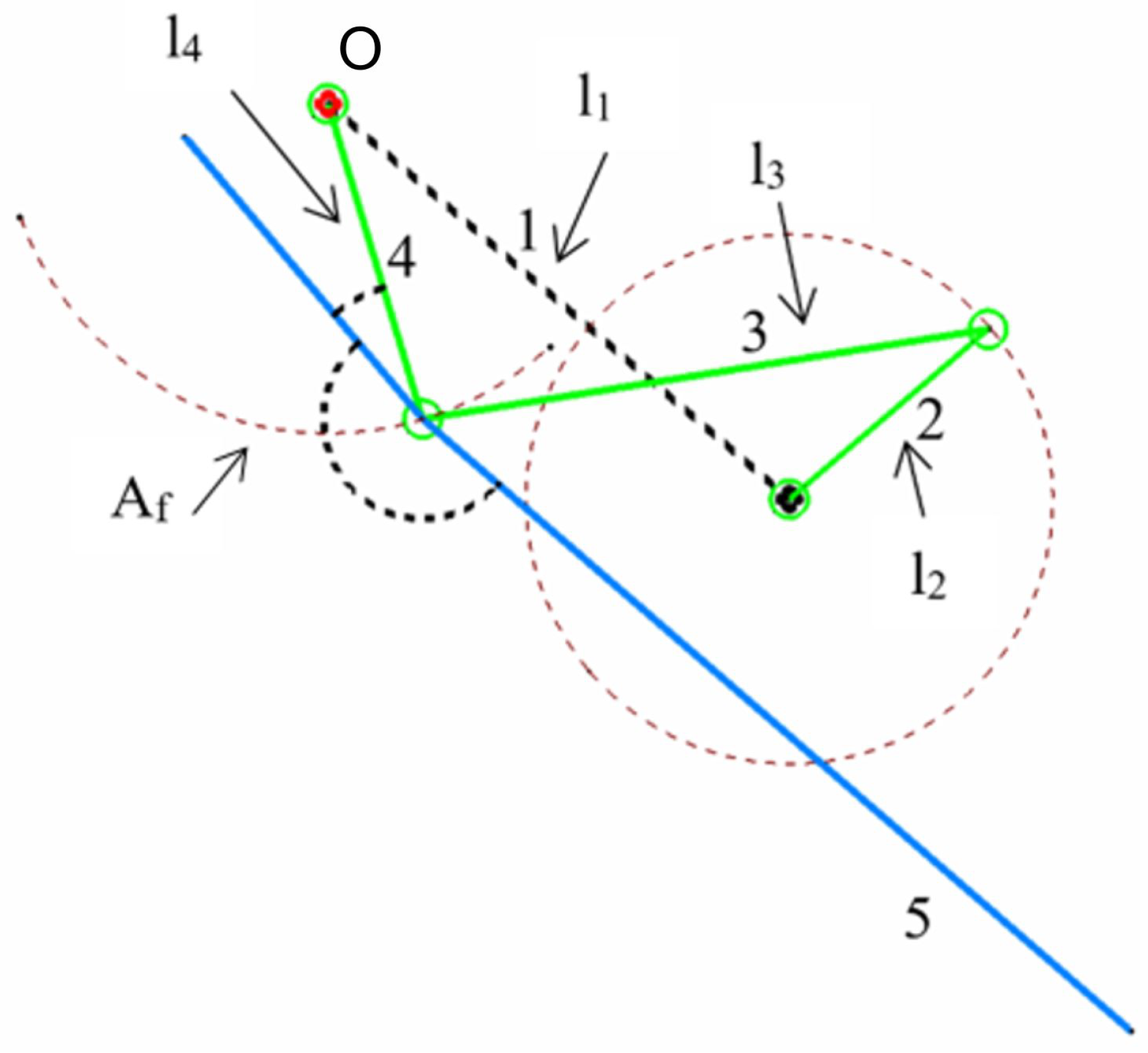
Figure 4.
Schematic representation of the flapping mechanism. The arrows indicate the design variables listed in
Table 3.
Figure 4.
Schematic representation of the flapping mechanism. The arrows indicate the design variables listed in
Table 3.
Figure 5.
Illustration of the basic layout of the mechanism inside the hull, and some geometrical requirements. The figure is not to scale.
Figure 5.
Illustration of the basic layout of the mechanism inside the hull, and some geometrical requirements. The figure is not to scale.
Figure 6.
Triangle arising from the geometrical simplification of the four-bar linkage mechanism. In the figure, the base of the triangle is equal to twice the length of the crank.
Figure 6.
Triangle arising from the geometrical simplification of the four-bar linkage mechanism. In the figure, the base of the triangle is equal to twice the length of the crank.
Figure 7.
Workflow of the iterative procedure used to approximate the lengths of the elements of the four-bar mechanism.
Figure 7.
Workflow of the iterative procedure used to approximate the lengths of the elements of the four-bar mechanism.
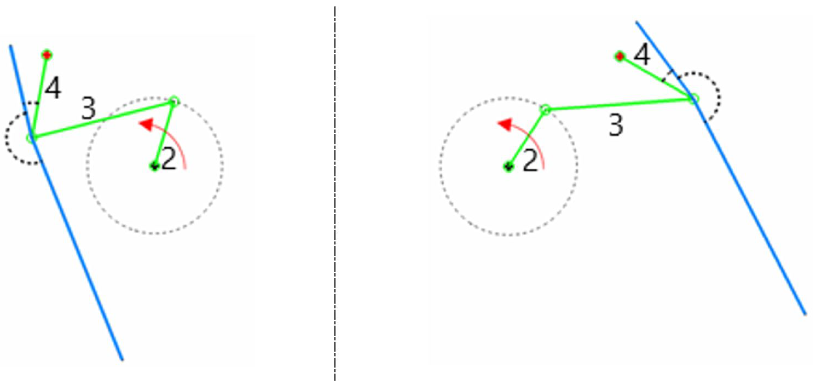
Figure 8.
Schematic representation of the left and right mechanisms. The red arrow indicates the sense of rotation of the crank. In the figure, the number 2 represents the crank, the number 3 represents the conrod, and the number 4 represents the rocker. The right mechanism is depicted at the maximum flapping angle, and the left mechanism is depicted at the minimum flapping angle.
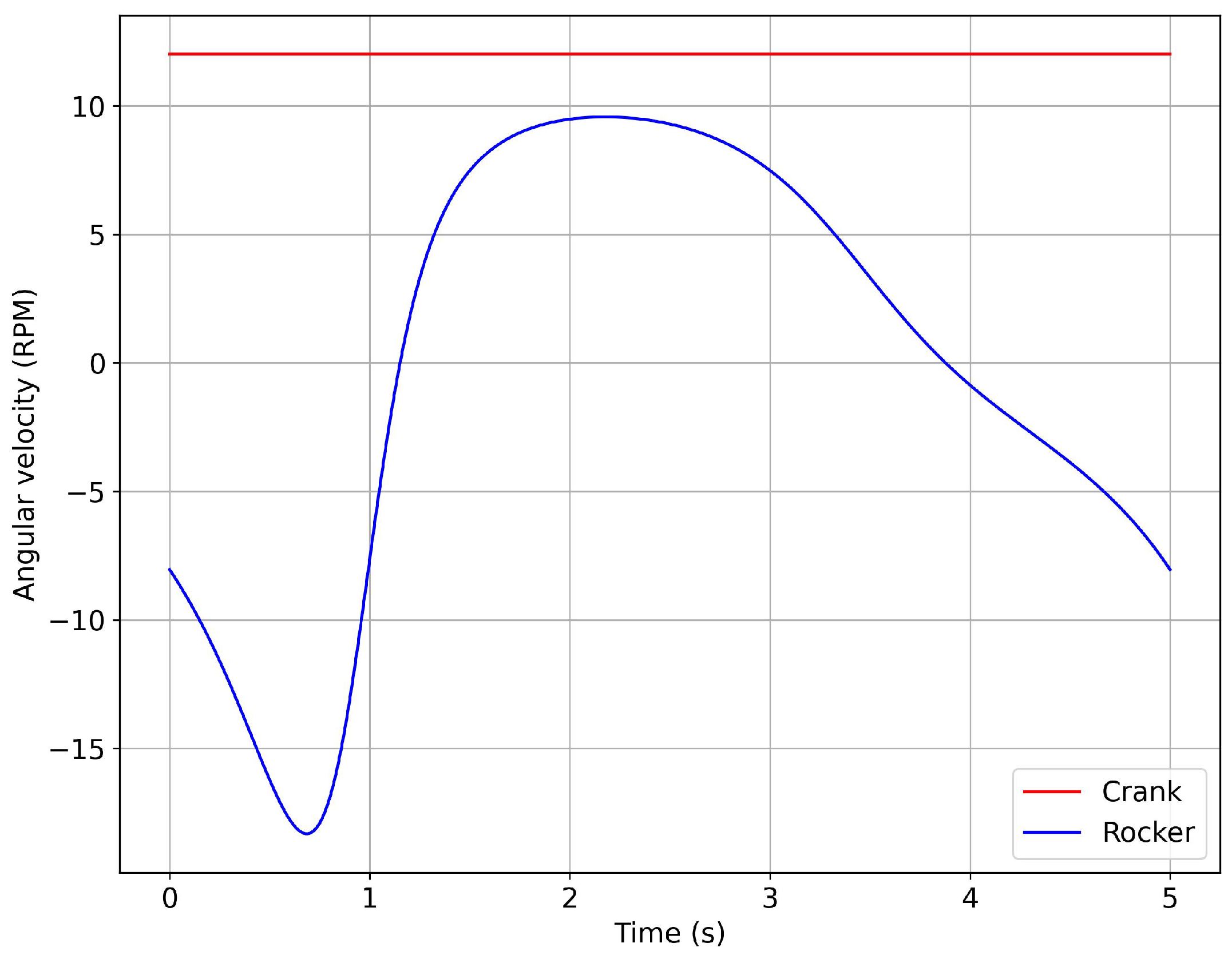
Figure 9.
Evolution of the angular velocity during one cycle of the flapping stroke. The blue line represents the rocker–fin component, and the red line represents the crank–motor assembly. The constant angular velocity of the crank–motor gave rise to the variable angular velocity of the rocker–fin.
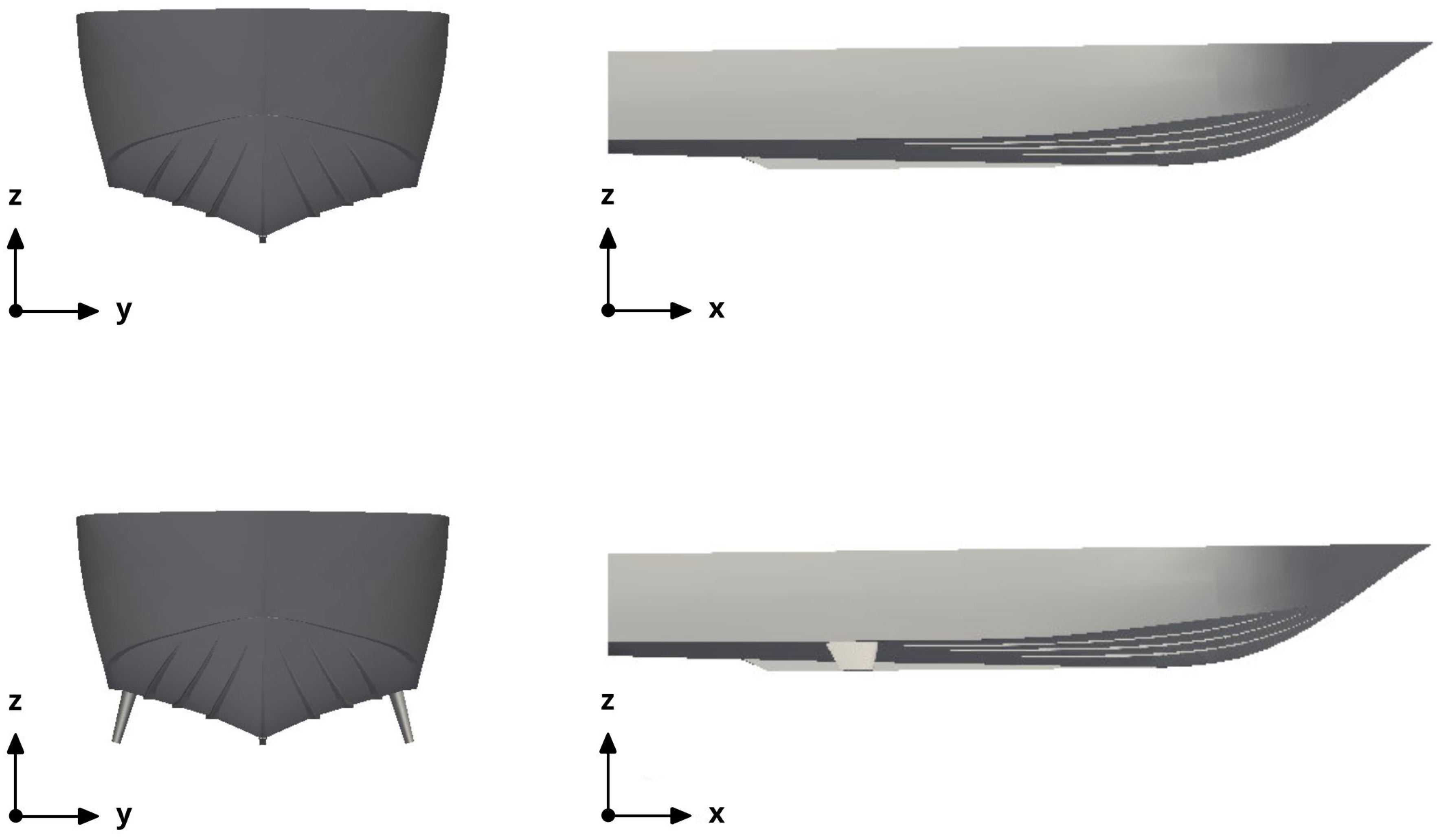
Figure 10.
Configurations studied. Top row: hull configuration with no fins. Bottom row: hull configuration with fixed fins.
Figure 10.
Configurations studied. Top row: hull configuration with no fins. Bottom row: hull configuration with fixed fins.
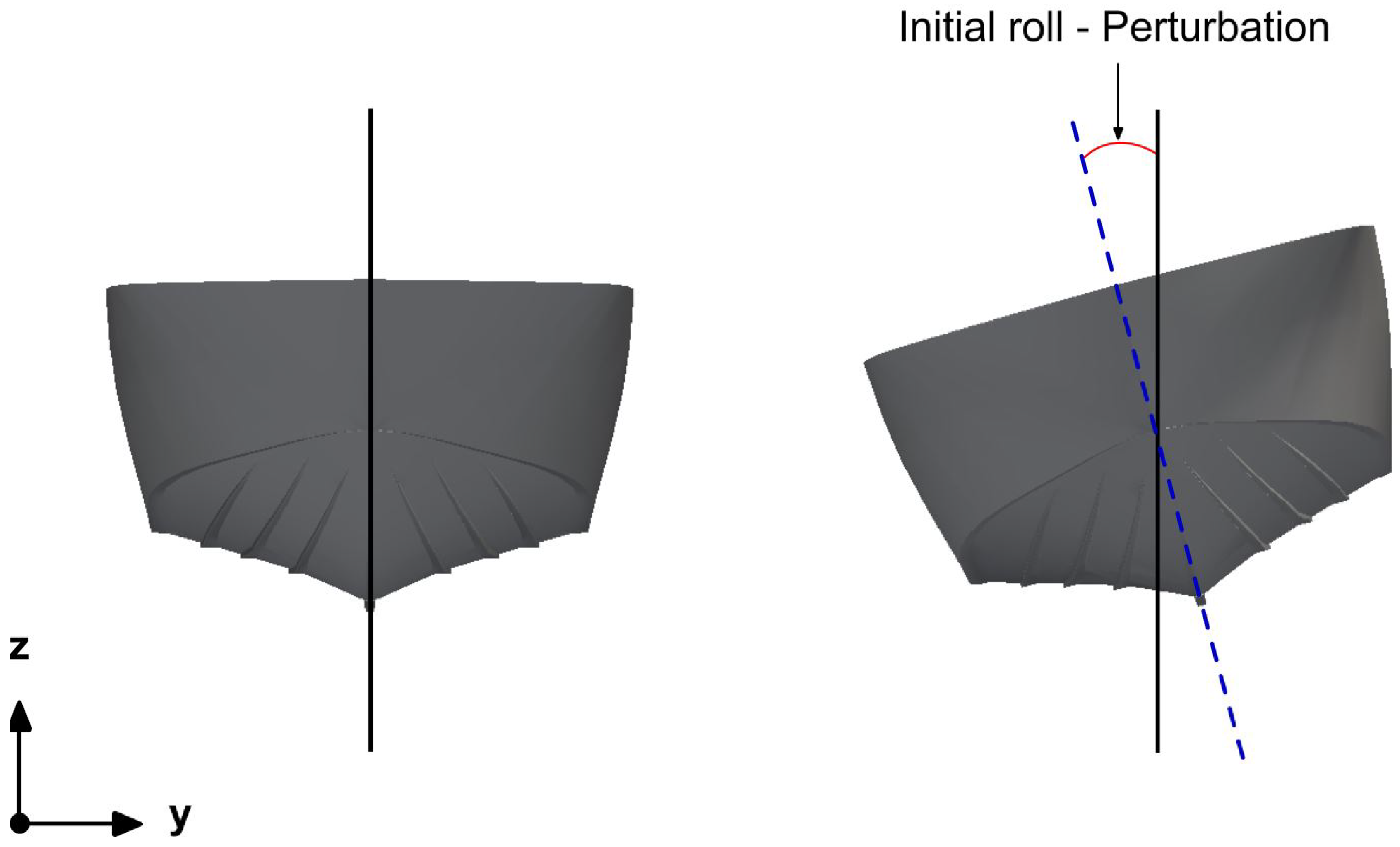
Figure 11.
Initial roll angle. The roll angle illustrated in the figure corresponds to 15 degrees.
Figure 11.
Initial roll angle. The roll angle illustrated in the figure corresponds to 15 degrees.
Figure 12.
Water level initialization (in cyan) at a roll angle equal to 15 degrees.
Figure 12.
Water level initialization (in cyan) at a roll angle equal to 15 degrees.
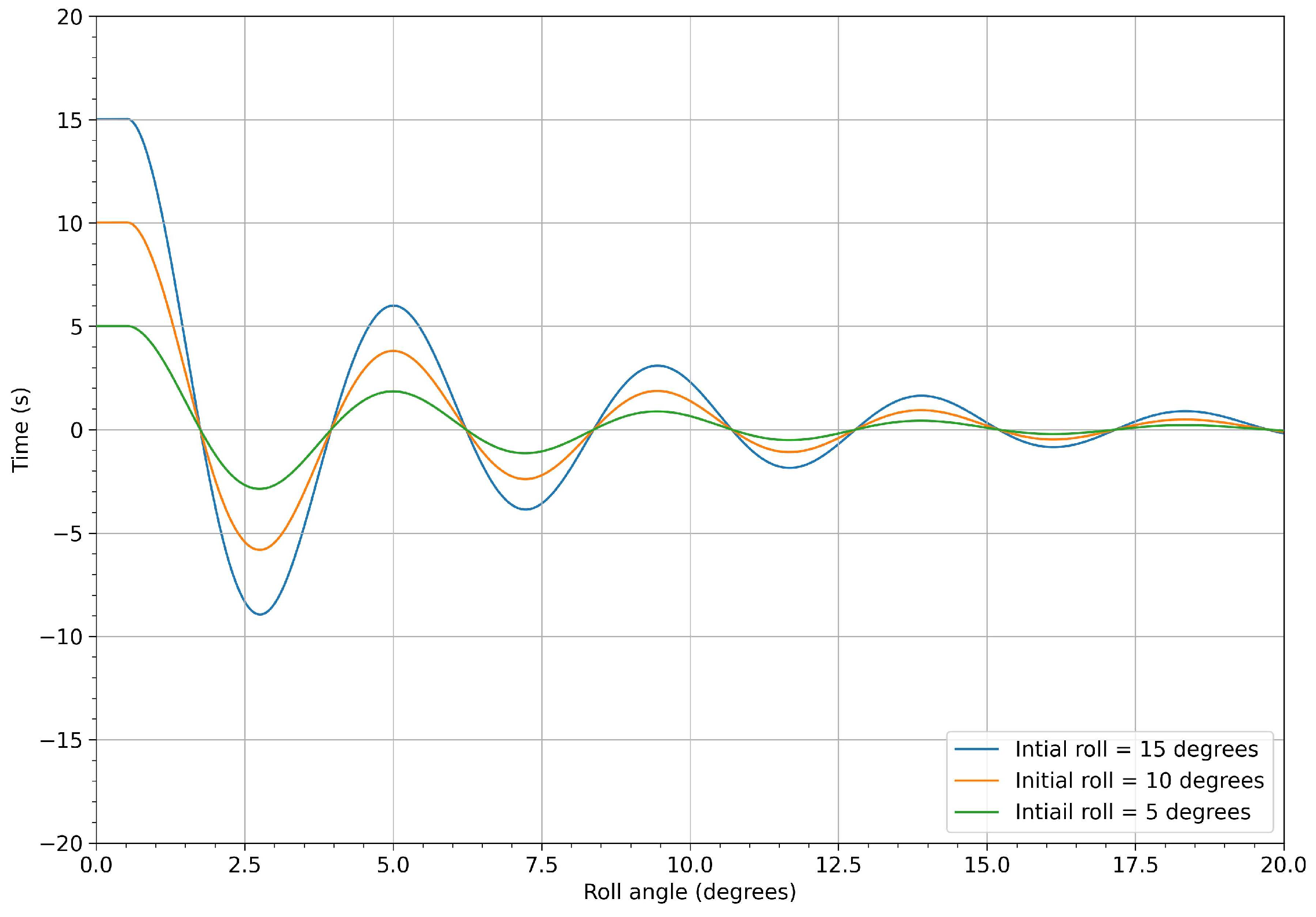
Figure 13.
Time evolution of the roll angle at different roll initial conditions for the configuration with no fins.
Figure 13.
Time evolution of the roll angle at different roll initial conditions for the configuration with no fins.
Figure 14.
Time evolution of the roll angle at different roll initial conditions for the model with fixed fins.
Figure 14.
Time evolution of the roll angle at different roll initial conditions for the model with fixed fins.
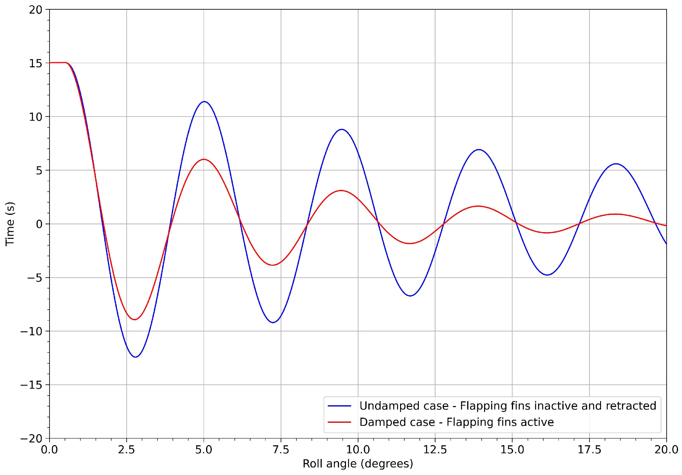
Figure 15.
Comparison of the time evolution of the roll angle for the configurations with no fins and with fixed fins: in both cases, the initial roll angle was equal to 5 degrees.
Figure 15.
Comparison of the time evolution of the roll angle for the configurations with no fins and with fixed fins: in both cases, the initial roll angle was equal to 5 degrees.
Figure 16.
Comparison of the time evolution of the roll angle for the configurations with no fins and with fixed fins: in both cases, the initial roll angle was equal to 15 degrees.
Figure 16.
Comparison of the time evolution of the roll angle for the configurations with no fins and with fixed fins: in both cases, the initial roll angle was equal to 15 degrees.
Figure 17.
Comparison of the damping frequency for the configurations with no fins and with fixed fins: in both cases, the initial roll angle was equal to 5 degrees.
Figure 17.
Comparison of the damping frequency for the configurations with no fins and with fixed fins: in both cases, the initial roll angle was equal to 5 degrees.
Figure 18.
Comparison of the damping frequency for the configurations with no fins and with fixed fins: in both cases, the initial roll angle was equal to 15 degrees.
Figure 18.
Comparison of the damping frequency for the configurations with no fins and with fixed fins: in both cases, the initial roll angle was equal to 15 degrees.
Figure 19.
Flapping fin geometry and location of rotation axis. The thickness of the flat plate was equal to 10 mm. The rotation axis corresponded to point 5 in
Figure 2. The figure is not to scale.
Figure 19.
Flapping fin geometry and location of rotation axis. The thickness of the flat plate was equal to 10 mm. The rotation axis corresponded to point 5 in
Figure 2. The figure is not to scale.
Figure 20.
Time evolution of the roll angle and angular velocity for a flapping frequency of 0.2 Hz.
Figure 20.
Time evolution of the roll angle and angular velocity for a flapping frequency of 0.2 Hz.
Figure 21.
Remeshing periods (vertical lines). The roll angle evolution shown in the figure corresponded to a flapping frequency of 0.2 Hz.
Figure 21.
Remeshing periods (vertical lines). The roll angle evolution shown in the figure corresponded to a flapping frequency of 0.2 Hz.
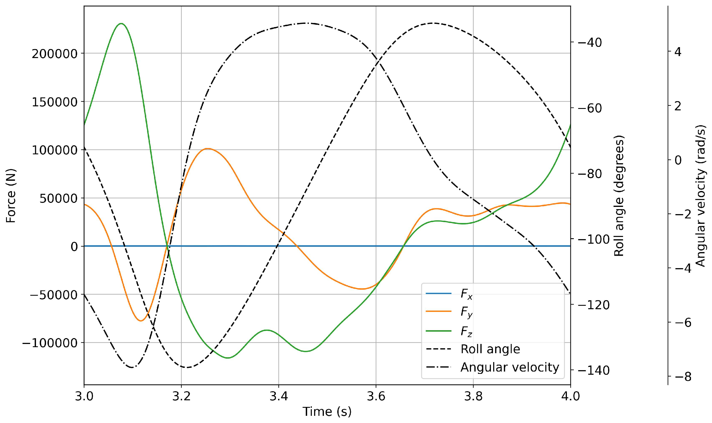
Figure 22.
Forces evolution during a flapping period (continuous lines). The dashed and dash–dot lines represent the roll angle and angular velocity, respectively. The flapping frequency was equal to 0.2 Hz.
Figure 22.
Forces evolution during a flapping period (continuous lines). The dashed and dash–dot lines represent the roll angle and angular velocity, respectively. The flapping frequency was equal to 0.2 Hz.
Figure 23.
Forces evolution during a flapping period (continuous lines). The dashed and dash–dot lines represent the roll angle and angular velocity, respectively. The flapping frequency was equal to 1.0 Hz.
Figure 23.
Forces evolution during a flapping period (continuous lines). The dashed and dash–dot lines represent the roll angle and angular velocity, respectively. The flapping frequency was equal to 1.0 Hz.
Figure 24.
Workflow used for the sizing and structural design of the components of the mechanism.
Figure 24.
Workflow used for the sizing and structural design of the components of the mechanism.
Figure 25.
Maximum and mean stresses on each component at different frequencies. In the figure, the circles represent the crank, the triangles represent the rocker, and the squares represent the conrod. The shaded symbols show the maximum stress, and the empty symbols show the mean stress. The dotted red line represents the upper threshold of the yield stress.
Figure 26.
Maximum stresses on each component at different frequencies. The circles represent the crank, the triangles represent the rocker, and the squares represent the conrod.
Figure 26.
Maximum stresses on each component at different frequencies. The circles represent the crank, the triangles represent the rocker, and the squares represent the conrod.
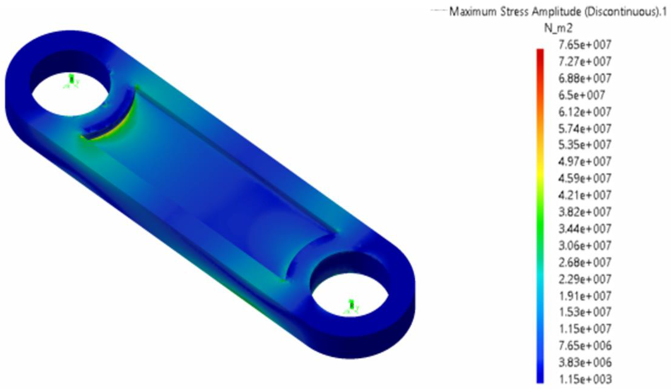
Figure 27.
Maximum stresses (Pa) on the conrod during the flapping cycle. Flapping frequency f = 0.2 Hz; maximum stress in the figure is equal to Pa.
Figure 27.
Maximum stresses (Pa) on the conrod during the flapping cycle. Flapping frequency f = 0.2 Hz; maximum stress in the figure is equal to Pa.
Figure 28.
Maximum deformation of the crank–conrod–rocker assembly, amplified by a factor of 100. Flapping frequency 0.2 Hz. The mesh used to conduct the structural analysis is also depicted.
Figure 28.
Maximum deformation of the crank–conrod–rocker assembly, amplified by a factor of 100. Flapping frequency 0.2 Hz. The mesh used to conduct the structural analysis is also depicted.
Figure 29.
Fatigue life in cycles for the Conrod at a flapping frequency equal to 0.2 Hz. In the figure, the number of cycles is very large, which indicates infinite durability.
Figure 29.
Fatigue life in cycles for the Conrod at a flapping frequency equal to 0.2 Hz. In the figure, the number of cycles is very large, which indicates infinite durability.
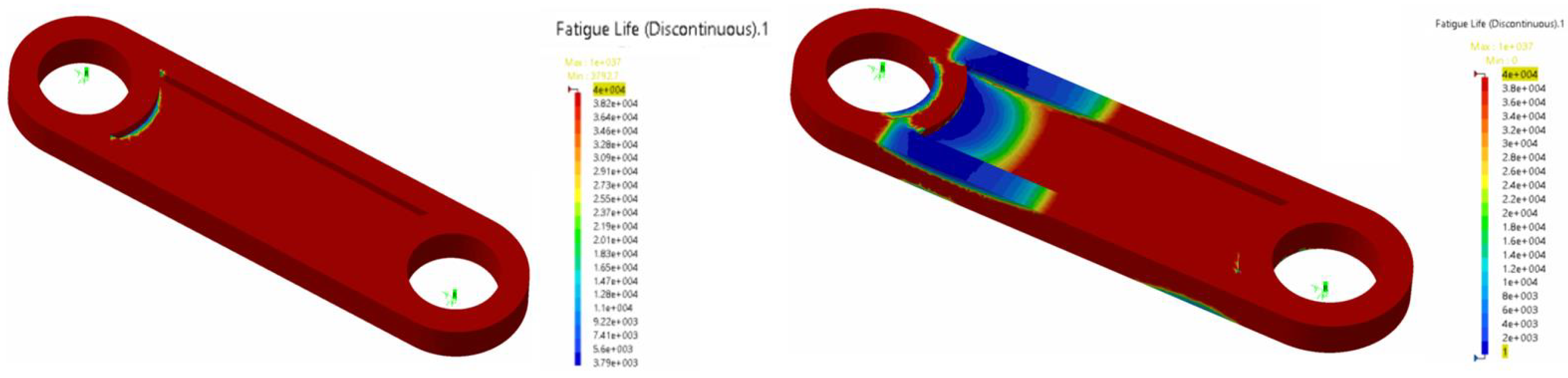
Figure 30.
(left image) fatigue life in cycles of the conrod at a flapping frequency of 0.25 Hz (infinite life). (right image) fatigue life of the conrod at a flapping frequency of 0.5 Hz (finite life). The component is likely to fail in the blue region at less than cycles.
Figure 30.
(left image) fatigue life in cycles of the conrod at a flapping frequency of 0.25 Hz (infinite life). (right image) fatigue life of the conrod at a flapping frequency of 0.5 Hz (finite life). The component is likely to fail in the blue region at less than cycles.
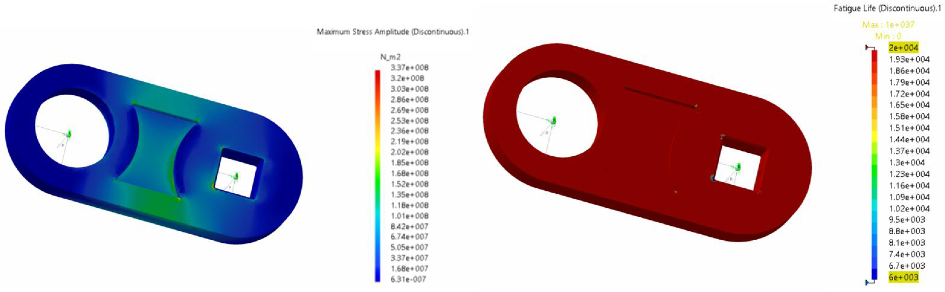
Figure 31.
Maximum stresses and fatigue life for the crank at a flapping frequency of 0.25 Hz. (left image) maximum stresses (maximum stress Pa). (right image) fatigue life in cycles. Note that the critical zones for fatigue life emerge in the area of the notches around the main pin.
Figure 31.
Maximum stresses and fatigue life for the crank at a flapping frequency of 0.25 Hz. (left image) maximum stresses (maximum stress Pa). (right image) fatigue life in cycles. Note that the critical zones for fatigue life emerge in the area of the notches around the main pin.
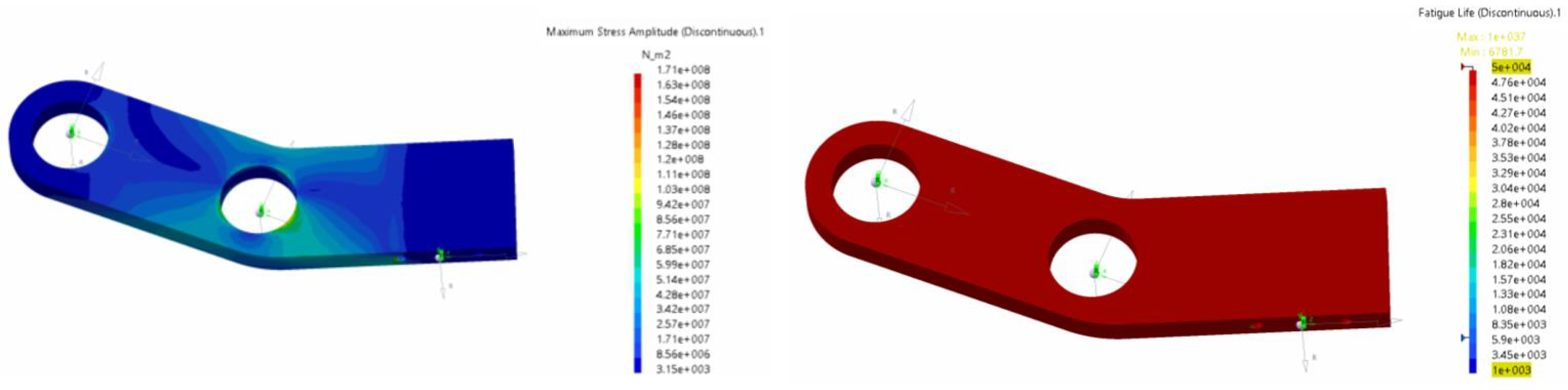
Figure 32.
Maximum stresses and fatigue life for the crank at a flapping frequency of 0.25 Hz. (left image) maximum stresses (maximum stress ). (right image) fatigue life in cycles. Note that a fatigue limited zone appears in the region where the rocker is connected to the fin.
Figure 32.
Maximum stresses and fatigue life for the crank at a flapping frequency of 0.25 Hz. (left image) maximum stresses (maximum stress ). (right image) fatigue life in cycles. Note that a fatigue limited zone appears in the region where the rocker is connected to the fin.
Figure 33.
Fatigue life of the crank–conrod–rocker assembly (drive mechanism) for a flapping frequency of 0.25 Hz (left image) and a flapping frequency of 0.5 Hz (right image).
Figure 33.
Fatigue life of the crank–conrod–rocker assembly (drive mechanism) for a flapping frequency of 0.25 Hz (left image) and a flapping frequency of 0.5 Hz (right image).
Figure 34.
Torque evolution of the motor for one flapping cycle. The blue line represents the rigid case (design condition) and the the red line represents the elastic case. The mean torque in both cases was approximately equal to 3500 (absolute value), and the peak torque was approximately 15,000 (absolute value).
Figure 35.
Instantaneous power evolution and mean power of the motor for one flapping cycle. The mean power was equal to 3.8 kW (absolute value). The peak power was approximately 18 kW (absolute value).
Figure 35.
Instantaneous power evolution and mean power of the motor for one flapping cycle. The mean power was equal to 3.8 kW (absolute value). The peak power was approximately 18 kW (absolute value).
Figure 36.
Roll angle evolution. The flapping frequency was equal to 0.2 Hz. Note that the starting roll angle was equal to 15 degrees (the maximum roll angle simulated using CFD).
Figure 36.
Roll angle evolution. The flapping frequency was equal to 0.2 Hz. Note that the starting roll angle was equal to 15 degrees (the maximum roll angle simulated using CFD).
Figure 37.
Roll angle evolution for three different initial conditions. The flapping frequency was equal to 0.2 Hz.
Figure 37.
Roll angle evolution for three different initial conditions. The flapping frequency was equal to 0.2 Hz.
Table 1.
Main characteristics and physical properties of the reference vessel. The vertical position of the center of gravity is measured in reference to the maximum depth of the vessel.
Table 1.
Main characteristics and physical properties of the reference vessel. The vertical position of the center of gravity is measured in reference to the maximum depth of the vessel.
| Parameter | Reference Value |
|---|
| Vessel displacement (D) | 90,000 kg |
| Waterline length () | 22.4 m |
| Maximum waterline beam () | 5.6 m |
| Draft (T) | 1.32 m |
| Vertical position of the center of gravity () | 2.46 m |
| Moment of inertia () | 600,000 kg·m |
Table 2.
Main design specifications used in this study.
Table 2.
Main design specifications used in this study.
| Vessel Characteristics | Value |
|---|
| Stabilization system available power () | 5.0 kW per fin |
| Natural roll frequency of the vessel () | 0.2 Hz |
| Maximum surface area of a single fin | 2.0 m |
Table 3.
Main geometrical characteristics of the mechanism. The corrected angle
was computed using the iterative process illustrated in
Figure 7.
Table 3.
Main geometrical characteristics of the mechanism. The corrected angle
was computed using the iterative process illustrated in
Figure 7.
| Geometrical Variable | Length (mm) | Angle |
|---|
| Frame length (fixed component) | 488 | - |
| Crank length | 210 | - |
| Conrod length | 460 | - |
| Rocker length | 264 | - |
| Corrected angle | - | |
Table 4.
Physical properties of the phases used in this study. The surface tension was equal to 0.072 N·m.
Table 4.
Physical properties of the phases used in this study. The surface tension was equal to 0.072 N·m.
| Phase | Density | Kinematic Viscosity |
|---|
| Water | 998.3 | |
| Air | 1.2 | |
Table 5.
Coefficients associated with Equation (
6). The coefficients listed in this table corresponded to a frequency of 0.2 Hz.
Table 5.
Coefficients associated with Equation (
6). The coefficients listed in this table corresponded to a frequency of 0.2 Hz.
| Coefficient Index n | | |
|---|
| 0 | −1.383 | – |
| 1 | −0.04723 | −0.8749 |
| 2 | 0.1189 | −0.03261 |
| 3 | 0.05942 | 0.01901 |
| 4 | 0.002404 | 0.01638 |
| 5 | −0.00536 | 0.007733 |
| 6 | −0.0029 | −0.0002547 |
| 7 | −0.0009761 | −0.0014 |
| 8 | 0.0002754 | −0.0005593 |
Table 6.
Mean values of the hydrodynamic forces.
Table 6.
Mean values of the hydrodynamic forces.
| Frequency (Hz) | Mean | Mean | Mean |
|---|
| 1.0 | 6.5 | 17,500 | 1200 |
| 0.7 | 1.9 | 9200 | 880 |
| 0.5 | 2.6 | 5100 | 450 |
| 0.333 | 1.8 | 2100 | 100 |
| 0.25 | 0.8 | 1300 | 90 |
| 0.2 | 0.4 | 80 | 60 |
Table 7.
Maximum values of the hydrodynamic forces.
Table 7.
Maximum values of the hydrodynamic forces.
| Frequency (Hz) | Max. | Max. | Max. |
|---|
| 1.0 | 90 | 121,990 | 233,880 |
| 0.7 | 30 | 55,530 | 113,390 |
| 0.5 | 20 | 31,560 | 63,380 |
| 0.333 | 12 | 13,830 | 26,640 |
| 0.25 | 6 | 7900 | 15,800 |
| 0.2 | 3 | 5320 | 10,540 |
Table 8.
Minimum values of the hydrodynamic forces.
Table 8.
Minimum values of the hydrodynamic forces.
| Frequency (Hz) | Min. | Min. | Min. |
|---|
| 1.0 | −42 | −80,200 | −12,7020 |
| 0.7 | −39 | −36,660 | −64,700 |
| 0.5 | −15 | −20,720 | −32,350 |
| 0.333 | −2 | −8990 | −14,270 |
| 0.25 | −1.5 | −5180 | −8090 |
| 0.2 | −2 | −3420 | −5500 |
Table 9.
Material physical properties. Standard steel.
Table 9.
Material physical properties. Standard steel.
| Physical Properties | Reference Value |
|---|
| Young modulus (E) | Pa |
| Poisson module () | 0.346 |
| Density () | 7680 kg/m |
| Yield strain () | 600–700 MPa |
| Ultimate strain () | 820 MPa |
Table 10.
Results of the structural analysis for each element of the mechanism at a frequency of 0.2 Hz.
Table 10.
Results of the structural analysis for each element of the mechanism at a frequency of 0.2 Hz.
| Component | Maximum Stress (MPa) | Maximum Displacement (mm) | / Ratio |
|---|
| Crank | 152 | 0.8324 | 3.95–4.61 |
| Conrod | 76.5 | 0.5674 | 7.84–9.15 |
| Rocker | 71.9 | 0.5179 | 8.34–9.74 |


