The Algebraic View of Computation: Implementation, Interpretation and Time

Abstract

Computational implementations are special relations between what is computed and what computes it. Though the word “isomorphism” appears in philosophical discussions about the nature of implementations, it is used only metaphorically. Here we discuss computation in the precise language of abstract algebra. The capability of emulating computers is the defining property of computers. Such a chain of emulation is ultimately grounded in an algebraic object, a full transformation semigroup. Mathematically, emulation is defined by structure preserving maps (morphisms) between semigroups. These are systematic, very special relationships, crucial for defining implementation. In contrast, interpretations are general functions with no morphic properties. They can be used to derive semantic content from computations. Hierarchical structure imposed on a computational structure plays a similar semantic role. Beyond bringing precision into the investigation, the algebraic approach also sheds light on the interplay between time and computation.

The steam engine replaced muscle power. It did not just make life easier, but a whole bunch of impossible things became possible. Curiously, it was invented before we understood how it worked. Afterward, trying to make it more efficient led to thermodynamics and indirectly to a deeper understanding of the physical world. Similarly, computers replace brain power, but we still do not have a full comprehension of computation. Trying to make computation more efficient and to find its limits is taking us to a deeper understanding of not just computer science, but of other branches of science (e.g., biology, physics, and mathematics). Just as physics advanced by focusing on the very small (particles) and on the very large (universe), studying computers should also focus on basic building blocks (finite state computations) and on large-scale abstract structures (hierarchical (de)compositions).

Another parallel with physics is that the underlying theory of computation is mathematical. Algebraic automata theory is a well-established part of theoretical computer science [1,2,3,4,5]. From a strictly technical point of view, it is not necessary to discuss computation at the algebraic level. Several excellent textbooks on the theory of computation do not even mention semigroups [6,7,8]. However, we argue here that for doing a more philosophical investigation of computation, semigroup theory provides the right framework.

The following theses summarize the key points of the algebraic view of computation:

• Computation has an abstract algebraic structure. Semigroups (sets with associative binary operation) are natural generalizations of models of computation (Turing machines, $\lambda$-calculus, finite state automata, etc.).
• Algebraic structure-preserving maps are fundamental for any theory of computers. Being a computer is defined as being able to emulate/implement other computers, i.e., being a homomorphic/isomorphic image. The rule of keeping the “same shape” of computation applies without exception, making programability and interactivity possible.
• Interpretations are more general functions than implementations. An arbitrary function without morphic properties can freely define semantic content for a computation. However, programability does not transfer to this level of semantics.
• Computers are finite. Finiteness renders decision problems trivial to solve, but computability with limited resources is a fundamental engineering problem that still requires mathematical research.
• Computers are general-purpose. They should be able to compute everything within their finite limits.
• Hierarchy is an organizing principle of computation. Artificial computing systems tend to have one-way (control) information flow for modularity. Natural systems with feedback loops also admit hierarchical models.

Here we reflect on the worldview, on the tacitly assumed ontological stance of a computational mathematician and software engineer, who is chiefly concerned with extending mathematical knowledge by enumerating finite structures. As such, we will mainly focus on classical digital computation and many aspects of computation (e.g., engineering practices and their social impacts) will not be discussed here. We will use only minimal mathematical formalism here; for technical details, see [9,10].

First we generalize traditional models of computation to composition tables that describe semigroups. We show how these abstract semigroups can cover the wide spectrum of computational phenomena. We then argue that homomorphisms, structure preserving maps between semigroups, together with finite universality, give the important concepts for defining computers. Lastly we mention how this fundamental theory can give rise to higher level of computational structures and touch upon several philosophical and more open-ended considerations.

1. Semigroup—Composition Table of Computations

Roughly speaking, computation is a dynamical process governed by some rules. This statement is general enough to be agreed upon.

“Abstract computers (such as finite automata and Turing machines) are essentially function-composition schemes.”

[11]

“Intuitively, a computing machine is any physical system whose dynamical evolution takes it from one of a set of ‘input’ states to one of a set of ‘output’ states.”

[12]

“A computation is a process that obeys finitely describable rules.”

[13]

“To compute is to execute an algorithm.”

[14]

But how to describe those rules? On the practical level of computation, we have different programming languages, and depending on the task, one is better suited than the others. Similarly, for the theoretical description of computation, depending on the purpose, one formalism might fit better than the other. Here we aim for the most general description with the purpose of being able to describe implementations in a simple way.

1.1. Generalizing Traditional Models of Computation

The Turing machine [15,16] is a formalization of what a human calculator or a mathematician would do when solving problems using pencil and paper. As a formalization, it abstracts away unnecessary details. For instance, considering the fact that we write symbols line by line on a piece of paper, the two-dimensional nature of the sheet can be replaced with a one-dimensional tape. Additionally, for symbolic calculations, the whole spectrum of moods and thoughts of a calculating person can be substituted with a finite set of distinguishable states. A more peculiar abstraction is the removal of the limits of human memory. This actually introduces a new feature: infinity (in the sense of capacity being unbounded). This is coming from the purpose of the model (to study decidability problems in logic) rather than the properties of a human calculator. Once we limit the tape or the number of calculation steps to a finite number, the halting problem ceases to be undecidable. In practice, we can do formal verification of programs. Therefore, to better match existing computers, we assume that memory capacity is finite. Such a restricted Turing machine is a finite state automaton (FSA) [1].

Now the FSA still has much that can be abstracted away. The initial and accepting states are for recognizing languages. The theory of formal languages is a special application of FSA. The output of the automaton can be defined as an additional function of the internal states, so we do not have to define output alphabet. What remains is a set of states, a set of input symbols, and a state transition function. An elementary event of computation is that the automaton is in a state, then it receives an input and based on that, it changes its state. We will show that the distinction between input symbols and states can also be abstracted away. It is important to note that FSA with a single input (e.g., clock-tick and the passage of time) are only a tiny subset of possible computations. Their algebraic structure is fairly simple. Metaphorically speaking, they are like batch processing versus interactivity.

1.2. Definition of Semigroups

What is then the most general thing we can say about computation? It certainly involves change. Turning input into output by executing an algorithm and going through many steps while doing so can be described as a sequence of state transitions. We can use the fundamental trick of algebra (writing letters to denote a whole range of possibilities instead of a single value) and describe an elementary event of computation by the equation as

$$xy=z.$$

Abstractly, we say that x is combined with y results in z. The composition is simply denoted by writing the events one after the other. One interpretation is that event x happens, then it is followed by event y, and the overall effect of these two events combined is the event z. Alternatively, x can be some input data and y a function; in the more usual notation, it would be denoted by $y\left(x\right)$. Or, the same idea with different terminology, x is a state and y is a state-transition operator. This explains how to compute. If we focus on what to compute, then we are interested only in getting the output from some input. In this sense, computation is a function evaluation, as in the mathematical notion of a function. We have a set of inputs, the domain of the function, and a set of outputs, the codomain. We expect to get an output for all valid inputs, and for a given input we want to have the same output whenever we evaluate the function. In practical computing, we often have “functions” that seem to violate these rules, so we distinguish between pure functions. A function call with a side effect (e.g., printing on screen) is not a mathematical function. This depends on how we define the limits of the system. If we put the current state of the screen into the domain of the function, then it becomes a pure function. For a function returning a random number, in classical computation, it is a pseudo-random number, so if we include the seed as another argument for the function, then again we have a pure function.

A single composition, when we put together x and y (in this order) yielding z, is the elementary unit of computation. These are like elementary particles in physics. In order to get something more interesting, we have to combine them into atoms. The atoms of computation will be certain tables of these elementary compositions, where two conditions are satisfied.

• The composition has to be associative,

  $$x\left(yz\right)=\left(xy\right)z,$$

  meaning that a sequence of compositions $xyz$ is well-defined.
• The table also has to be self-contained, meaning that the result of any composition should also be included in the table. Given a finite set of n elements, the $n\times n$ square table will encode the result of combining any two elements of the set.

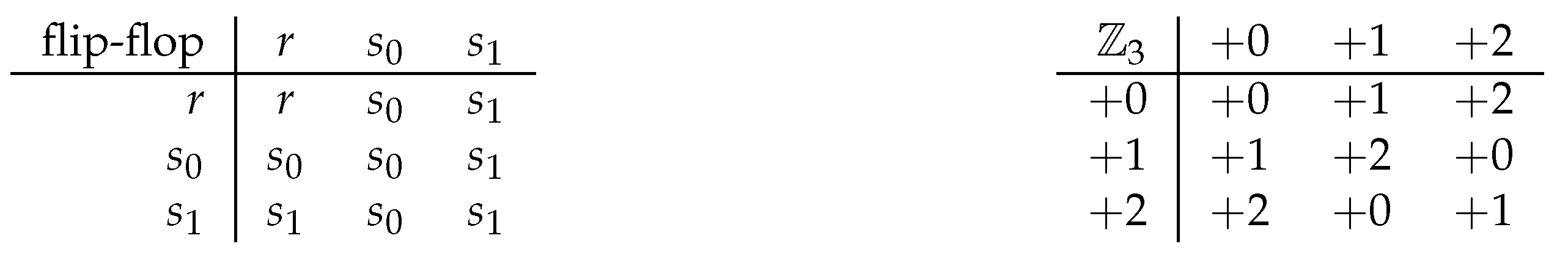
The underlying algebraic structure is called the semigroup (a set with an associative binary operation, [17]), and the composition is often called multiplication (due to its traditional algebraic origin) or the Cayley table (Figure 1). Continuing the physical metaphor, not all composition tables are atoms, as some tables are built by using simpler tables (as we will discuss later).

Talking about state transitions, we still do not say anything concrete about the states. If state changes along a continuum, then we talk about analog computing. If state is a discrete configuration, then we have classical computing. In case we have a vector of amplitudes, then we have quantum computing. Additionally, $xy$ in itself is a sequential composition, but y can be a parallel operation. We will see that concurrency and parallelism are more specific details of computations.

Is the distinction between states and events fundamental? The algebraic thinking guides the abstraction. The number 4 can be identified with the operation of adding 4, relative to 0, so it is both a state and an operation.

Principle 1 (State-event abstraction).

We can identify an event with its resulting state: state x is where we end up when event x happens, relative to a ground state. The ground state, in turn, corresponds to a neutral event that does not change any state.

Semigroups can be infinite with their composition tables going to infinity in both dimensions. The reason why we insist on finiteness is that we want to use them to measure computational power.

“Numbers measure size, groups measure symmetry.”

[18]

The general idea of measuring is that we assign a mathematical object to the thing to be measured. In the everyday sense, the assigned object is a number, but for measuring more complicated properties, we need more structured objects. In this sense, we say that semigroups measure computation. Turing completeness is just a binary measure, hence the need for a more fine-grained scale [10]. Thus, we can ask questions like “What is the smallest semigroup that can represent a particular computation?”

1.3. Computation as Accretion of Structure

The classical (non-interactive) computation admits an interesting characterization: generating structures from partial descriptions. The archetypical example is a sudoku puzzle with a unique solution [19], where the accretion of the structure is visual. In solving a puzzle, we progress by putting more numbers into the table, determined by the pre-filled configuration. More general examples are graph search algorithms, where the graph is actually created during the search. Logical inference also fits this pattern: the premises determine the conclusions through intermediate expressions. Even when we only keep the final result as a single data item, we still generate intermediate data (structure). The existing entries (input) implicitly determine the whole table (output), but we have to execute an algorithm to find those entries. As a seed determines how a crystal grows, the input structure determines the whole. This is absolute determinism. In a sense, the full structure is already there when we execute an algorithm that generates it from a partial description. As we will discuss, this has an interesting interplay with time.

This idea of accretion has a clear algebraic description: the set of generators. These are elements of a semigroup whose combinations can generate the whole table. In order to calculate the compositions of generators, they have to have some representation. For instance, transformations of a finite set with n elements. A transposition, a full cycle, and an elementary collapsing can generate all possible $n^n$ transformations. For a more general computation, the executable program and the input data together serve as a generating set, or the primitives of a programming language can take that role [20].

2. Computation and Time

Time is a big mystery in physics, despite the fact the it is “everywhere” as we seem to live in it. Similarly, computation has become pervasive in our life, but we still lack a thorough understanding of computational processes. It is no surprise that these two have a rich and tangled relationship.

2.1. Different Times

The most immediate observation about mechanized computation is that it happens on a time scale completely different from compared to the human conscious thinking process. If we could peek into the working processor of a desktop computer, we would see nothing. First, the electrons are invisible, but even if photons were used to carry information, we could only see some faint glow, since the bit-flips were so frequent. If we could slow down the computer, to the extent that we could see the bits in the processor registers flipping, then how much time would it take to process the event of a key press? Another extreme difference between logical time and actual time is that computation can be suspended.

2.2. Not Enough Time

Staying in the realm of computable problems, much of practical computing and most of computer science is about calculating something as fast as possible, given some finite resources. Due to finiteness, we always have a working algorithm, since we can apply a brute force algorithm for answering a question by simply going through all possible answers systematically, keeping an eye out for the right solution(s). The problem is the time needed for the execution.

If there were infinite time available for computation, or equivalently, infinitely fast computers, we would not need to do any programming at all, brute-force would suffice (time travel even changes computability [21]). This is a neglected part of time travel science fiction stories. A possible shortcut to the future would render the P vs. NP problem meaningless with enormous consequences (which were explored separately in [22]).

2.3. Timeless Computation?

When a computational experiment is set up and the programmer hits the ENTER key, all that separates her from knowing the answer is time. The execution time is crucial for our computations. Computational complexity classifies algorithms by their space and time requirements. Memory space can often be exchanged for time and the limit of this process is the lookup table, the precomputed result. Taking the abstraction process to its extreme, we can replace the two-dimensional composition table with a one-dimensional lookup table, with keys as pairs $(x,y)$ and values $xy$. This formal trick brings the idea of a giant immutable table containing the results of all possible computations of a particular computer. Computation, completely stripped off any locality the process may have, is just an association of keys to values. This explains why arrays and hashtables are important data structures in programming. The composition table is just an unchanging array, so all computations of a computing device have a timeless interpretation as well. Here we do not want to go into the several interpretations of time (for the two extremes, see [23,24]); we wish only to emphasize that computation is orthogonal to the problem of time. We can talk about static computational structures, composition tables, and we can also talk about computational processes, sequences of events tracing a path in the composition table.

What makes the execution time issue particularly frustrating is the absolute determinism of a classical computer. A computer is similar to a bread maker. You first put flour, water, salt, and yeast in. Then, assuming that electricity will remain available, a few hours later, one will have a warm, fresh smelling loaf. Once the button is pressed, the home appliance is bound to bake bread. The chemical properties of water and flour and the biological properties of yeast determine the speed of the bread making process. One can choose a faster program, but the result will then not be as tasty. For computation, the speed is determined by the physical properties of electricity, by the chemical properties of silicon; and it is ultimately determined by the energy constraints.

We showed that computation can be defined in a timeless way. It turns out that the two extremes span a whole continuum, where static and procedural information are exchangeable. The slogan is as follows: If computation is information processing, then information is frozen computation. For instance, for a Rubik’s Cube, I can specify a particular state either by describing the positions and orientations of the cubelets or by giving a sequence of moves from the initial ordered configuration. This is another example of the state-event abstraction (Principle 1).

3. Homomorphism—The Algebraic Notion of Implementation

The biggest gain from the algebraic definition of computation is that structure preserving maps between computing devices are straightforward to define. The main message of this paper is that, for talking about a computer emulating another, abstract algebra is the right language. It also gives a clear definition of a computer.

The importance of the relation between what is computed with what computes was recognized before computers existed. Ada Lovelace called it the uniting link, which is the idea of implementation.

“In enabling mechanism to combine together general symbols in successions of unlimited variety and extent, a uniting link is established between the operations of matter and the abstract mental processes of the most abstract branch of mathematical science.”

[25]

Implementation cannot be just loosely defined as some arbitrary correspondence. Without the precision of algebra, it becomes possible to talk about computing rocks and walls, pails of water (for an overview of pancomputationalism, see [26]).

“A physical system implements a given computation when the causal structure of the physical system mirrors the formal structure of the computation.”

[27]

This statement captures the crucial idea of implementation, but the language of a finite state automata makes the explanation unnecessarily complicated [14,27,28].

3.1. Homomorphisms

Homomorphism is a simple concept, but its significance can be hidden in the algebraic formalism. The etymology of the word conveys the underlying intuitive idea: the ancient Greek ὁμός (homos) means “same,” and μορφή (morphe) means “form” or “shape”. Thus, homomorphism is a relation between two objects when they have the same shape. The abstract shape is not limited to static structures. We can talk about homomorphisms between dynamical systems, i.e., finding correspondences between states of two different systems and for their state transition operations as well. Change in one system is mimicked by the change in another. Homomorphism is a knowledge extension tool: we can apply knowledge about one system to another. It is a way to predict outcomes of events in one dynamical system based on what we know about what happens in another one, given that a homomorphic relationship has been established. This is also a general trick for problem solving, widely used in mathematics. When obtaining a solution is not feasible in one problem domain, we can use easier operations by transferring the problem to another domain—assuming that we can move between the domains with structure preserving maps.

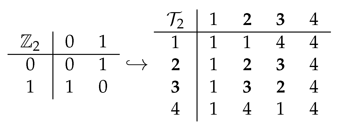
What does it mean to be in a homomorphic relationship for computational structures? Using the composition table definition, we can now define their structure preserving maps. If in a system S event x combined with event y yields the event $z=xy$, then by a homomorphism $\phi :S\to T$, then in another system T the outcome of $\phi \left(x\right)$ combined with $\phi \left(y\right)$ is bound to be $\phi \left(z\right)=\phi \left(xy\right)$, so the following equation holds

$$\phi \left(xy\right)=\phi \left(x\right)\phi \left(y\right).$$

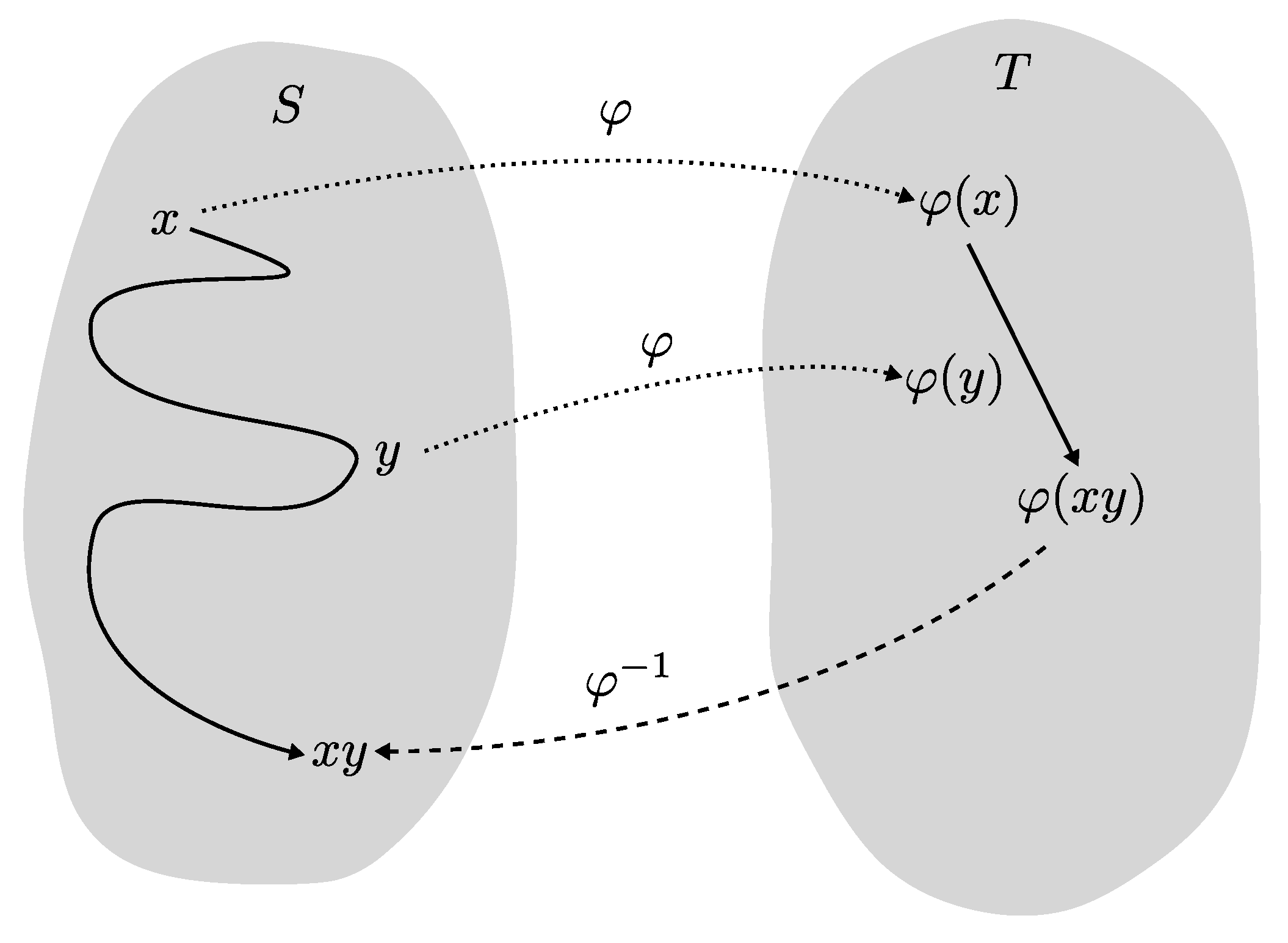
On the left hand side, composition happens in S, while on the right hand side composition is done in T (see Figure 2 for a concrete example and Figure 3 for a visualization of locating composition). What is the typical usage of the homomorphism? Let’s say I want to compute $xy$, where x can be some input data and y a function. But I cannot just apply the function, because it would be impossible to do it in my head or it would take a long time to do it on sheets of paper with a pen. But I have some physical system T, whose internal dynamics is homomorphic to how the function works. So I represent x in T as $\phi \left(x\right)$, and y as $\phi \left(y\right)$, then let the dynamics of T carry out the combination of $\phi \left(x\right)\phi \left(y\right)$. By the homomorphism, that is the same as $\phi \left(xy\right)$. At the end I need to find out how to map the result back to $xy$. The classic example is the use of logarithm tables for computing products of large numbers. There is a strict relationship between the addition of exponents and the multiplication of numbers, which can be exploited for speeding up numerical calculations.

What makes homomorphism powerful is that it is systematic. It works for all combinations not just a one-off correspondence. There is no way to opt out: the rule has to work not just for a single sequence but for all possible sequences of events, for the whole state-transition table. Otherwise, one could fix an arbitrary long computation as a sequence of state transitions. Then, by a carefully chosen encoding, any physical system with enough states can execute the same sequence. But the same encoding will be unlikely to work for a different sequence of state transitions, thus it is not a homomorphism.

A distinguished class of homomorphisms are isomorphisms, where the correspondence is one-to-one. In other words, isomorphisms are strictly structure preserving, while homomorphisms can be structure forgetting down to the extreme of mapping everything to a single state and to the identity operation. The technical details can be complicated due to clustering states (surjective homomorphism) and by the need of turning around homomorphism we also consider homomorphic relations [9,10].

By turning around implementations we can define computational models. We can say that a physical system implements an abstract computer, or we can say that the abstract computer is a computational model of the physical system. These notions are relative, so we might become unsure about the directions.

“…we need to discover whether the laws of physics are prior to, in the sense of constraining, the possibilities of computation, or whether the laws of physics are themselves consequences of some deeper, simpler rules of step-by-step computation.”

[29]

At least in science fiction, one can turn physical reality vs. mathematical description relation around. In a fictional story mathematical truth (about abstract structures) depends on what computers actually calculate.

“‘A mathematical theorem,’ she’d proclaimed, ‘only becomes true when a physical system tests it out: when the system’s behaviour depends in some way on the theorem being true or false.”’

“‘…And if a mathematician could test those steps by manipulating a finite number of physical objects for a finite amount of time—whether they were marks on paper, or neurotransmitters in his or her brain—then all kinds of physical systems could, in theory, mimic the structure of the proof…with or without any awareness of what it was they were proving.’”

[30]

3.2. Computers as Physical Systems

The point of building a computer is that we want the computation done by a physical system on its own, just by supplying energy. So if a computational structure as a mathematical entity determines the rules of computation, then somehow the physical system should obey those rules. This crucial idea has been formulated several times.

“Computing processes are ultimately abstractions of physical processes: thus, a comprehensive theory of computation must reflect in a stylized way aspects of the underlying physical world.”

[31]

“Our computers do no more than re-program a part of the universe to make it compute what we want it to compute.”

[32]

“A computer is an arrangement of some of the material constituents of the Universe into a configuration whose natural evolution in time according to the laws of Nature simulates some mathematical process.”

[29]

“…the universal computer can eventually do what any other computer can. In other words, given enough time it is universal.”

[33]

“In a sense, nature has been continually computing the ‘next state’ of the universe for billions of years; all we have to do—and, actually, all we can do—is ‘hitch a ride’ on this huge ongoing computation, and try to discover which parts of it happen to go near to where we want.”

[31]

“Computation: A physical process that instantiates properties of some abstract entity.”

[34]

The essence of these informal definitions is the idea of structure preserving maps. Therefore, within the semigroup formalism, the definition of computers is easy to state.

Definition 1 (vague).

Computers are physical systems that are homomorphic images of computational structures (semigroups).

This first definition begs the question, how can a physical system be an image of a homomorphism, i.e., a semigroup itself? How can we cross the boundary between the mathematical realm and the external reality? First, there is an easy but hypothetical answer. According to the Mathematical Universe Hypothesis [35,36], all physical systems are mathematical structures, so we never actually leave the mathematical realm.

“Our external physical reality is a mathematical structure.”

[35]

Secondly, the implementation relation can be turned around. Implementation and modeling are the two directions of the same isomorphic relation. If T implements S, then S is a computational model of T. Again, we stay in the mathematical realm, we just need to study mappings between semigroups. Establishing and verifying a computational model of a physical system require scientific work (both theoretical and experimental) and engineering. The computational model of the physical system may not be complete. For instance, classical digital computation can be implemented without quantum mechanics. To emphasize the connection between implementation and modeling, we can give an improved definition of computers.

Definition 2.

Computers are physical systems whose computational models are homomorphic images of semigroups.

This definition of computers is orthogonal to the problem of whether mathematics is an approximation or a perfect description of physical reality, and the definition does not depend on how physical systems are characterized.

For practical purposes, we are interested in implementations of computational structures that are in some sense universal. In the finite case, for n states, we require the physical system be able to implement ${\mathcal{T}}_n$, the full transformation semigroup of n states. These mathematical objects contain all possible state transformations of a state set of a given size. Thus, for each n, we have a finite analogue for Turing-completeness. This measure roughly translates into memory size, but the subsemigroups of the full transformation semigroups offer an even more fine-grained measure.

Every dynamical system computes something, at least its future states. The question is whether we can make a system compute something useful for us, as well as how much useful computation the system can perform. In the steam engine, every water molecule has some kinetic energy, but not all of them happen to bump into the piston. All others generate only waste heat by banging on the walls of the cylinder. Similarly, it is not easy to find dynamical systems that do computation that is useful for us. We have to design and engineer those. A piece of rock is unchanging on the macro level, so it only implements the identity function. On the microscopic level, it can be used for computing random numbers by measuring the vibration of its atoms. But it is not capable of universal computation. Only carefully crafted pieces of rock, the silicon chips, can have this very special property.

Biological systems are also good candidates for hosting computation, since they’re already doing some information processing. However, it is radically different from digital computation. The computation in digital computers is like toppling dominoes, a single sequence of chain reactions of bit-flips. Biological computation is done in a massively parallel way (e.g., all over in a cell), more in a statistical mode.

Alternatively, we can redefine the computational work we want to do. If it is a continuous mathematical problem, then it is easy to find a physical system that is capable of the corresponding analogue computation.

3.3. Difficulty in Programming

Philosophical discussions often focus on embedding minds into computers. However, the other direction is also important. Computer science education is interested in how we can play out programs in our head. When we program, what are we doing exactly? First, we need to imagine a computational process we want to create. Second, we have to code that into a particular language.

The coding part is easier, since programming languages are smaller and by design simpler than natural languages. Therefore, the difficulty must be in the imagination part.

Imagining computation means playing out a symbolic mechanism in our head. Our brain is the runtime, and we execute the code in our thinking. When writing assembly code, we envision bit-flips in registers and track data moving between memory and the processor. In object-oriented programming, we have to picture the interaction patterns in the relation network of objects. In functional programming, we have to visualize the structure of function calls and the substitution of arguments.

We emulate the computer by thinking about the running code. Which computer exactly? This is a nontrivial question, which turns out to be a crucial one in computing education research. It is called a “notional machine,” defined as “an abstract computer responsible for executing programs of a particular kind.” [37]. In other words, there is a morphic relation between the computation happening in the computer and our thoughts. Today, almost any computer can recreate the behaviour of 8-bit computers from the 1980s. That is not surprising at all. A more powerful machine can emulate a less powerful one, simply by having more memory and faster processors to make up for any difference between the machines. However, the other way around, trying to emulate a computer with less resources, difficulties arise. This is what happens when we program.

The brain is a very lousy digital computer. It cannot focus strictly on a single data item. It is more like an association machine: when one thought arises, many other thoughts come into play. It also has severe limitations in scalability. The great thing about computers is that they do things very fast and can process a huge number of data items. We can keep only a small number of thoughts in our minds at a time. We can imagine small cases, but errors might pop up for greater instances of problems. We are also not too good in exploring all combinatorial possibilities, we tend to check the familiar cases. That’s why we need to generate our test cases. The brain has vast resources, but they are of a different type and often biased evolutionary and culturally.

3.4. Interpretations

Computational implementation is a homomorphism, while an arbitrary function with no homomorphic properties is an interpretation. We can take a computational structure and assign freely some meaning to its elements, which we can call the semantic content. Interpretations look more powerful since they can bypass limitations imposed by the morphic nature of implementations. However, since they are not necessarily structure preserving, the knowledge transfer is just one way. Changes in the underlying system may not be meaningful in the target system. If we ask a new question, then we have to devise a new encoding for the possible solutions.

For instance, reversible system can carry out irreversible computation by a carefully chosen output encoding [10,31]. A morphism can only produces irreversible systems out irreversible systems (algebraically: the image of a group homomorphism is a group). This in turn demonstrates that today’s computers are not based on the reversible laws of physics. From the logic gates up, we have proper morphic relations, but the gates themselves are not homomorphic images of the underlying physics. When destroying information, computers dissipate heat. Whether we can implement group computation with reversible transformations and hook on a non-homomorphic function to extract semantic content is an open engineering problem [38]. In essence, the problem of reversible computation implementing programs with memory erasure is similar to trying to explain the arrow of time arising from the symmetrical laws of physics.

4. High-Level Structure: Hierarchies

“Computers are built up in a hierarchy of parts, with each part repeated many times over.”

[39]

Composition and lookup tables are the “ultimate reality” of computation, but they are not adequate descriptions of practical computing. The low-level process in a digital computer, the systematic bit flips in a vast array of memory, is not very meaningful. The usefulness of a computation is expressed at several hierarchical layers above (e.g., computer architecture, operating system, and end user applications). Parallel computation and interactive processes can also be described as gigantic composition tables. However, they have more explanatory power when viewed by the rules of their communication protocol. Algebraic identities can describe the multitude of computational events efficiently. In the form of equations, we can express laws that are universal (e.g., associativity) or specific to a particular computer.

A semigroup is seldom just a flat structure, its elements may have different roles. For example, if $xy=z$ but $yx=y$ (assuming $x\ne y\ne z$), then we say that x has no effect on y (leaves it fixed), while y turns x into z. There is an asymmetric relationship between x and y: y can influence x but not the other way around. This unidirectional influence give rise to hierarchical structures. It is actually better than that. According to the Krohn–Rhodes theory [40], every automaton can be emulated by a hierarchical combination of simpler automata. This is true even for inherently non-hierarchical automata built with feedback loops between its components. It is a surprising result of algebraic automata theory that recurrent networks can be rolled out to one-way hierarchies. These hierarchies can be thought as easy-to-use cognitive tools for understanding complex systems [41]. They also give a framework for quantifying biological complexity [42].

The simpler components of a hierarchical decomposition are roughly of two kinds. Groups correspond to reversible combinatorial computation. Groups are also associated with isomorphisms (due to the existence of unique inverses), so their computation can also be viewed as pure data conversion. Semigroups, which fail to be groups, contain some irreversible computation, i.e., destructive memory storage.

5. Wild Considerations

It is natural to ask whether the mind is computational or not, however it may be a bit too early. We simply do not know enough about it yet. Computation is already fascinating, even without being able to explain our thinking processes. Still, we can consider the question.

The algebraic theory of implementing computations is a description of what we have in today’s computers. It is not known whether the semigroup computation model can explain the mind, but there is not much left to abstract from it. Thus, the question of whether cognition is computational or not, might be the same as the question of whether mathematics is a perfect description of physical reality or is just an approximation of it. If it is just an approximation, then there is a possibility that cognition resides in physical properties that are left out.

A recurring question in philosophical conversations is the possibility of the same physical system realizing two different minds simultaneously [43]. Let’s say n is the threshold for being a mind. You need at least n states for a computational structure to do so. Then supposedly there is more than one way to produce a mind with n states, so the corresponding full transformation semigroup ${\mathcal{T}}_n$ can have subsemigroups corresponding to several minds. We then need a physical system to implement ${\mathcal{T}}_n$. Now, it is a possibility to have different embeddings into the same system, so the algebra might allow the possibility of two minds coexisting in the same physical system. However, it also implies that most subsystems will be shared or we need a bigger host with at least $2n$ states. If everything is shared, the embeddings can still be different, but then a symmetry operation could take one mind into the other. This is how far mathematics can go in answering this question.

For scientific investigation, these questions are still out of scope. Simpler questions about the computation form a research program [10]. For instance, What is the minimum number of states to implement a self-referential system? and, more generally, What are the minimal implementations of certain functionalities? and How many computational solutions are there for the same problem? These are engineering problems, but solutions for these may shed light on the more difficult questions about the possibilities and constraints of embedding cognition and consciousness into computers.

6. Summary

Here we brought together algebraic automata theory, a somewhat neglected part of theoretical computer science, and philosophical considerations on what constitutes a computer. The underlying mathematics, semigroup theory, provides a suitable language in which the notion of computational implementation can be defined in a simple way. Algebraic structure preserving maps spread “computerness” from one system to the other, and full transformation semigroups are the preimages of general-purpose computers. The semigroup model of computers also provides ways for giving semantics to computations (interpretations and hierarchical structures) and flexibility for accommodating different theories of time.

In our opinion, philosophy should be ahead of mathematics, as it deals with more difficult questions, and it should not be bogged down by the shortcomings of terminology. In philosophy, we want to deal with the inherent complexity of the problem, not the incidental complexity caused by the chosen tool. The algebraic viewpoint provides a solid base for further philosophical investigations of the computational phenomena.