Effects of Symmetry Breaking in Resonance Phenomena

Abstract

We show that resonance phenomena can be treated as nonequilibrium phase transitions. Resonance phenomena, similar to equilibrium phase transitions, are accompanied by some kind of symmetry breaking and can be characterized by order parameters. This is demonstrated for spin-wave resonance, helicon resonance, and spin-reversal resonance.

1. Introduction

The great majority of phase transitions are characterized by spontaneous symmetry breaking and can be described by the qualitative changes in the order parameter behavior associated with long-range order [1,2]. This concerns both first-order as well as second-order phase transitions. There are also so-called topological phase transitions [3] that are not necessarily accompanied by symmetry breaking, but exhibit the changes in the behavior of correlation functions and of reduced density matrices, connected with a kind of quasi-long-range or mid-range order [4]. In all cases, even when order parameters cannot be defined, different phases can be classified by order indices of density matrices [5,6,7,8] quantifying all types of order, be they long-range or mid-range.

Phase transitions between equilibrium states of matter are induced by the variation in thermodynamic parameters or static external fields. Similarly, the appearance of new properties in a nonequilibrium system can be induced by alternating fields, especially when some resonances occur.

In the present paper, we advocate the point of view that resonance phenomena can be treated as nonequilibrium phase transitions. As in the case of equilibrium phase transitions, resonance phenomena are accompanied by qualitative changes in their macroscopic properties, which makes it possible to introduce related order parameters. In many cases, resonance phenomena exhibit a kind of symmetry breaking. We illustrate these properties by considering several resonances for which we define the related order parameters and show that this kind of symmetry can become broken. As examples, we consider spin-wave resonance, helicon resonance, and spin-reversal resonance.

Let us emphasize that we do not claim that resonance phenomena are exactly the same as equilibrium phase transitions. This is evidently not so, since resonance phenomena describe nonequilibrium processes. However, we show that both these phenomena can share two, probably the most important, properties: First, there can occur some symmetry breaking in a region around the resonance. Second, it is possible to introduce order parameters distinguishing between qualitatively different states of the considered system. These similarities justify the comparison between resonance phenomena and phase transitions.

We do not prescribe in advance what would be the order of transition in particular resonance phenomena. As always, this is defined by the behavior of the related order parameters. The realistic description of resonance phenomena is usually dealt with finite systems, since, to realize a resonance, one always needs an alternating external field, created outside of and acting on the system. For finite systems, the problem of thermodynamic limit does not arise at all. Dealing with finite systems, it is natural to expect that the related resonance transitions will be of continuous type, analogous to transformations in finite equilibrium systems. In the majority of cases, transitions caused by resonances are in fact crossover transitions.

An exact resonance, as such, happens at a single point of a varied parameter, usually of frequency. However, this does not mean that the transition is localized at that single point. As we shall see from the examples below, there is a region around the point of the exact resonance where new properties, compared to those in the regions far from the resonance point, arise. Such a region, which can be called the resonance region, reminds us of the critical region in equilibrium phase transitions.

Again let us stress that resonance phenomena are nonequilibrium, and symmetry breaking, generally, drives systems to nonuniform states. The most convenient way of describing such systems is by considering the dynamics of observable quantities that are defined through the corresponding statistical averages. All examples, we consider below, are based on exactly this approach of studying the dynamic behavior of observable quantities. The dynamical equations in all cases are derived from related microscopic theories. Of course, it would be absolutely unreasonable to reproduce all these rather complicated derivations in the present paper. This could take hundreds of pages, especially for realistic problems we deal with. Instead, it is sufficient in the present paper to give the appropriate references where the reader can find all details.

Throughout the paper, we set the Planck constant to unity.

2. Spin-Helicon Waves

First, we consider resonances that occur in a paramagnetic metal subject to the irradiation of an external electromagnetic field. The metal is assumed to have the geometry of a plate in the region $0<z<L$. There is an external static magnetic field along the z axis,

$${\mathbf{B}}_0=B_0{\mathbf{e}}_z$$

(1)

and perpendicularly to its surface the metal is irradiated by an alternating electromagnetic field of frequency $\omega$ much lower than the plasma frequency,

$$\omega \ll {\omega }_p\left({\omega }_p^2\equiv 4\pi \frac{\rho e_0^2}{m}\right)$$

(2)

where $\rho \sim {10}^{22}$ cm${}^{-3}$, $e_0$, and m are the electron density, charge, and mass, respectively. The plasma frequency is ${\omega }_p\sim {10}^{15}$ s${}^{-1}$. The static paramagnetic susceptibility in paramagnetic metals is small, so that

$$4\pi \chi \ll 1.$$

(3)

Usually, the susceptibility is of order $\chi \sim {10}^{-6}$.

The excitation of waves inside a metallic plate is achieved in the best way by circularly polarized electromagnetic waves [9,10], because of which we consider the electromagnetic fields and magnetic moment in the form of the combinations

$$H=H_x-i{H}_y,E=E_x-i{E}_y,M=M_x-i{M}_y.$$

(4)

The temporal behavior is described by $exp(-i\omega t)$.

The coupled Maxwell–Bloch equations for linear field deviations in a paramagnetic metal with weak dispersion and isotropic Fermi surface can be written [11,12,13,14,15] as

$$\begin{gathered} \frac{dH}{dz}-\varepsilon kE=0,\frac{dE}{dz}+k(H+4\pi M)=0 \\ \left(D\frac{d^2}{d{z}^2}-{\omega }_s+i{\nu }_s\right)(M-\chi H)+\omega M=0. \end{gathered}$$

(5)

Here, $k\equiv \omega /c$, the effective dielectric permeability is

$$\varepsilon =-\frac{{\omega }_p^2}{\omega (\omega -{\omega }_s+i{\nu }_0)}$$

(6)

and the diffusion coefficient reads as

$$D=\frac{v_F^2(1+{\beta }_0)(1+{\beta }_1)}{3(\omega -{\omega }_0+i{\nu }_0)}$$

(7)

where

$${\omega }_s=\frac{e_0{B}_0}{mc}$$

(8)

is the Larmor spin frequency, and the cyclotron frequency

$${\omega }_0=\frac{1+{\beta }_1}{1+{\beta }_0}{\omega }_s$$

(9)

is renormalized by the Landau Fermi-liquid interaction parameters ${\beta }_0$ and ${\beta }_1$. The attenuations

$${\nu }_s=\frac{1+{\beta }_0}{{\tau }_s},{\nu }_0=\frac{1+{\beta }_1}{{\tau }_0}$$

(10)

are defined by the times of momentum, ${\tau }_0\sim {10}^{-9}$ s, and spin, ${\tau }_s\sim {10}^{-6}$ s, relaxations. The Fermi velocity of conduction electrons is $v_F\sim {10}^8$ cm s${}^{-1}$. Equation (5) describe the coupled spin-helicon waves with the dispersion relation

$$q^2=\varepsilon \mu (q,\omega )$$

(11)

where the effective magnetic permeability is

$$\mu (q,\omega )=\frac{\omega -{\omega }_s+i{\nu }_s-D{q}^2}{\omega +(1-4\pi \chi )(-{\omega }_s+i{\nu }_s-D{q}^2)}.$$

(12)

This gives us two solutions for the characteristic wave vectors, associated with the spin waves, $k_s$, and helicon waves, $k_h$. Taking into account the smallness of the static paramagnetic susceptibility, we can write

$$k_s^2=\frac{\omega -{\omega }_s+i{\nu }_s}{D},k_h^2=\varepsilon k^2(4\pi \chi \ll 1)$$

(13)

to zero order in $\chi$, and

$$\begin{gathered} k_s^2=\frac{\omega -{\omega }_s+i{\nu }_s}{D}\left(1+\frac{4\pi \chi \omega }{\omega -{\omega }_s+i{\nu }_s-D\varepsilon k^2}\right) \\ {k}_h^2=\varepsilon k^2\left(1+4\pi \chi \frac{-{\omega }_s+i{\nu }_s-D\varepsilon k^2}{\omega -{\omega }_s+i{\nu }_s-D\varepsilon k^2}\right) \end{gathered}$$

(14)

to first order in $\chi$.

The incident and reflected fields are plane waves, with the magnetic components

$$H_0(z)=H_0{e}^{ikz},H_1(z)=H_1{e}^{-ikz}(z\le 0),$$

(15)

which defines the total magnetic field $H_0(z)+H_1(z)$. Respectively, the electric components yield the electric field

$$E_0(z)+E_1(z)=i[H_0(z)-H_1(z)](z\le 0).$$

(16)

Inside the metallic plate, the magnetic field consists of four parts, including two running waves and two waves reflected from the second surface of the plate,

$$H(z)=H_2{e}^{i{k}_{s}z}+H_3{e}^{-i{k}_{s}z}+H_4{e}^{i{k}_{h}z}+H_5{e}^{-i{k}_{h}z}(0\le z\le L).$$

(17)

The field transmitted through the second surface is

$$H_6(z)=H_6{e}^{ikz},E_6(z)=i{H}_6(z)(z\ge L).$$

(18)

Equation (5) are to be complimented by the boundary conditions. For magnetic and electric fields, there are the standard continuity conditions for their tangential components on each of the surfaces. The spatial structure of the metallic surface influences the spatial distribution function of conducting electrons [16]. This can result in the appearance of a magnetic anisotropy on the surface. Several boundary conditions for the magnetization have been studied [17,18,19,20,21,22]. A simple boundary condition for the magnetization was proposed by Dyson [23], which reads as

$$\frac{dM}{d\mathbf{n}}+\zeta M=0(z=0,L)$$

(19)

where the first term implies the normal derivative at the boundary and $\zeta$ is a surface anisotropy parameter connected to the probability of a spin flip when scattering at the surface. The Dyson boundary condition has been used in several papers [18,24,25,26]. Experiments have not been able to determine between the preferred type of condition [27,28]. Hence, without the loss of generality, we can employ the Dyson condition (19). The six boundary conditions at two surfaces, for the fields and for the magnetic moment, define all six amplitudes $H_i$, with $i=1,2,3,4,5,6$ as functions of the incident-field amplitude $H_0$.

A convenient observable quantity is the transparency coefficient

$$C_T\equiv {\left|\frac{H_6}{H_0}\right|}^2$$

(20)

showing how the incident electromagnetic field is transmitted through the metallic plate.

3. Spin-Wave Resonance

When the frequency $\omega$ of the incident field is close to the spin frequency ${\omega }_s$, the helicon amplitudes $H_4$ and $H_5$ are small, as compared to the spin-wave amplitudes $H_2$ and $H_3$, and the spin wave forms a standing wave, so that the magnetic field inside the plate becomes practically periodic, slightly perturbed by attenuations. Respectively, the magnetic moment is also practically periodic:

$$M(z)\propto cos(k_{s}z).$$

(21)

This looks like a kind of magnetic crystallization of spin-wave collective excitations, whereby the system becomes spatially periodic if a small attenuation is neglected.

For typical paramagnetic metals, the spin frequency is ${\omega }_s\sim {10}^{11}$ s${}^{-1}$, the wave vectors are $k_s\sim {10}^2$ cm${}^{-1}$ and $k_h\sim {10}^6$ cm ${}^{-1}$, and the magnetic anisotropy parameter is $\zeta \sim {10}^3$ cm${}^{-1}$. The plate width is typically $L\sim {10}^{-2}$ cm. Hence the inequalities

$$|k_s|\ll \zeta \ll |k_h\left|\right|k_{h}L|\gg 1$$

(22)

are valid, which will be used in what follows. Employing these inequalities, we obtain the transparency coefficient

$$C_T=\frac{64{\pi }^2{\chi }^2{\omega }^2{|k_s|}^2}{c^2{\zeta }^6{|sin(k_{s}L)|}^2}(\omega \sim {\omega }_s).$$

(23)

In the denominator,

$$|sin(k_{s}L){|}^2={sin}^2(\mathrm{Re}{k}_{s}L)+{sinh}^2(\mathrm{Im}{k}_{s}L)$$

where

$$\mathrm{Re}{k}_s=|k_s|cos\phi ,\mathrm{Im}{k}_s=\left|k_s\right|sin\phi ,$$

and $\phi$ is the argument of $k_s$. Thus, we have

$$C_T\propto \frac{{\omega }^2{\left|k_s\right|}^2{L}^2}{{sin}^2(|k_{s}L|cos\phi )+{sinh}^2(|k_{s}L|sin\phi )}$$

(24)

where

$$|k_{s}L|=\frac{\sqrt{3}}{v_F}{\left\{\frac{[{(\omega -{\omega }_s)}^2+{\nu }_s^2][{(\omega -{\omega }_0)}^2+{\nu }_0^2]}{{(1+{\beta }_0)}^2{(1+{\beta }_1)}^2}\right\}}^{1/4}$$

(25)

and the phase is

$$\phi =\frac{1}{2}arctan\left[\frac{{\nu }_0(\omega -{\omega }_s)+{\nu }_s(\omega -{\omega }_0)}{(\omega -{\omega }_s)(\omega -{\omega }_0)-{\nu }_0{\nu }_s}\right].$$

(26)

The spin-wave resonance occurs under the condition

$$\mathrm{Re}{k}_{s}L=\left|k_{s}L\right|cos\phi =\pi n(n=1,2,\dots ).$$

(27)

To simplify the formulas, we can take into account that the Fermi-liquid interaction parameters ${\beta }_0$ and ${\beta }_1$ are small and that dimensionless attenuations

$${\nu }_1\equiv \frac{{\nu }_0}{{\omega }_s},{\nu }_2\equiv \frac{{\nu }_s}{{\omega }_s}.$$

(28)

In typical paramagnetic metals, ${\nu }_0\sim {10}^9$ s${}^{-1}$, ${\nu }_s\sim {10}^6$ s${}^{-1}$, and ${\omega }_s\sim {10}^{11}$ s${}^{-1}$. Therefore, ${\nu }_1\sim {10}^{-2}$ and ${\nu }_2\sim {10}^{-5}$. In view of these small parameters, we have

$$|k_s|\simeq \frac{\sqrt{3}}{v_F}(\omega -{\omega }_s).$$

Thus, the resonance condition (27) yields the spin-resonance frequencies

$${\omega }_n={\omega }_s\left(1+\frac{An}{cos\phi }\right)(n=1,2,\dots )$$

(29)

in which

$$A\equiv \frac{\pi v_F}{\sqrt{3}L{\omega }_s}.$$

(30)

For the typical values $v_F\sim {10}^8$ cm s${}^{-1}$ and $L\sim {10}^{-2}$ cm, the parameter $A\sim 0.1$ and $\phi \sim {10}^{-2}$. Hence,

$$\phi \simeq \frac{1}{2}arctan\left(\frac{{\nu }_1+{\nu }_2}{An}\right).$$

(31)

In what follows, we consider the first resonance, with $n=1$, whose frequency is

$${\omega }_1={\omega }_s(1+A)$$

(32)

where we take into account that, because of the smallness of $\phi$, $cos\phi \approx 1$.

Introducing the relative detuning

$$\delta \equiv \frac{\omega -{\omega }_1}{{\omega }_1}$$

(33)

we can write

$$|k_{s}L|=\pi (1+b\delta )\left(b\equiv \frac{1+A}{A}\right).$$

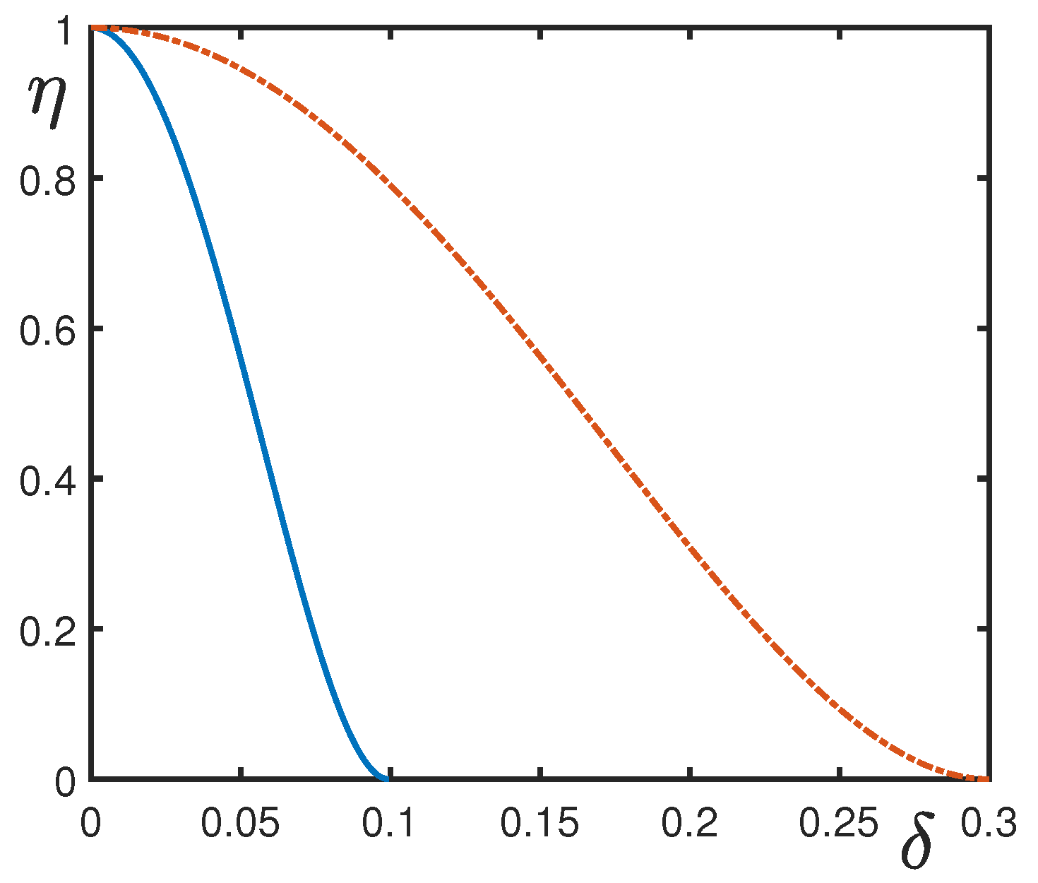
The occurrence of spin-wave resonance manifests itself by the appearance of the well observable property of the transparency of the metallic plate with respect to the penetration of electromagnetic waves. The order parameter can be defined as the normalized transparency coefficient

$$\eta \equiv \frac{C_T(\delta )}{C_T(0)}.$$

(34)

For the latter, we obtain

$$\eta =\frac{{(1+\delta )}^2{(1+b\delta )}^2{sinh}^2(\pi sin\phi )}{{sin}^2[\pi (1+b\delta )cos\phi ]+{sinh}^2[\pi (1+b\delta )sin\phi ]}.$$

(35)

The order parameter (Equation (35)), as a function of the relative detuning, is shown in Figure 1. In the vicinity of the resonance frequency, where the detuning is close to zero, the order parameter is close to one. In addition, it diminishes with increasing the detuning.

The state at small detuning is qualitatively different from the state far from $\delta =0$. The sample under spin-wave resonance becomes periodic due to the developed standing wave (21), and the plate exhibits the macroscopic property of transparency. These features disappear outside of the resonance. Such behavior reminds us of a phase transition.

4. Helicon Resonance

At a frequency $\omega$ much lower than the spin frequency ${\omega }_s$,

$$\omega \ll {\omega }_s$$

(36)

spin waves strongly attenuate, but helicon waves can persist [29,30]. At such frequencies, the transparency coefficient (20) becomes

$$C_T=\frac{4\omega {\omega }_s}{{\omega }_p^2{|sin(k_{h}L)|}^2}$$

(37)

where

$$k_h=\sqrt{\varepsilon }\frac{\omega }{c},\varepsilon =\frac{{\omega }_p^2({\omega }_s+i{\nu }_0)}{\omega ({\omega }_s^2+{\nu }_0^2)}.$$

(38)

The real and imaginary parts of the helicon wave vector are

$$\mathrm{Re}{k}_h=\frac{{\omega }_p}{c}\sqrt{\frac{\omega }{{\omega }_s}}cos\phi ,\mathrm{Im}{k}_h=\frac{{\omega }_p}{c}\sqrt{\frac{\omega }{{\omega }_s}}sin\phi$$

(39)

with the argument

$$\phi =\frac{1}{2}arctan\frac{{\nu }_0}{{\omega }_s}.$$

(40)

From the transparency coefficient

$$C_T=\frac{4\omega {\omega }_s}{{\omega }_p^2[{sin}^2(\mathrm{Re}{k}_{h}L)+{sinh}^2(\mathrm{Im}{k}_{h}L)]}$$

(41)

it follows that the helicon resonance happens when

$$\mathrm{Re}{k}_{h}L=\pi n(n=1,2,\dots ).$$

(42)

The helicon resonance frequencies, keeping in mind that ${\nu }_0/{\omega }_s\sim {10}^{-2}$, is read as

$${\omega }_n=\frac{{\pi }^2{c}^2{\omega }_s{n}^2}{{\omega }_p^2{L}^2{cos}^2\phi }(n=1,2,\dots ).$$

(43)

We shall consider the first resonance with the frequency

$${\omega }_1={\left(\frac{\pi c}{{\omega }_{p}L}\right)}^2{\omega }_s.$$

(44)

This frequency is of order ${\omega }_1\sim {10}^6$ s${}^{-1}$.

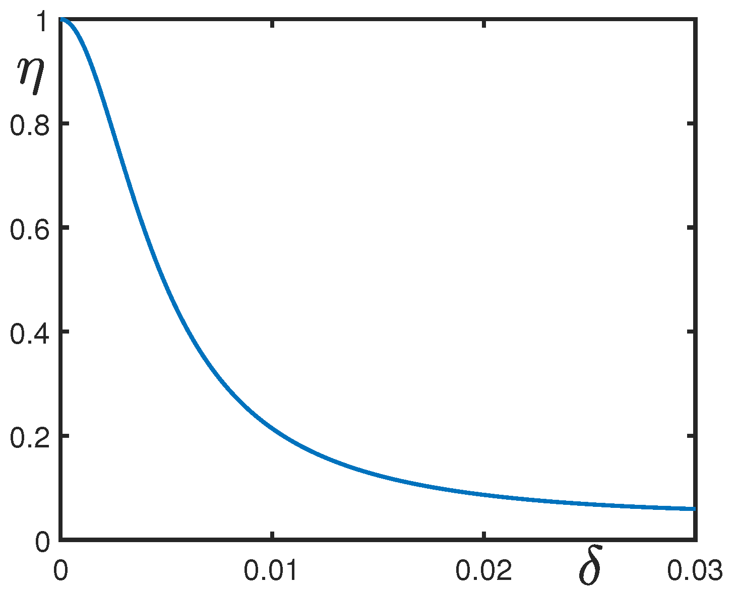
The order parameter can again be defined as the normalized transparency coefficient

$$\eta \equiv \frac{C_T(\delta )}{C_T(0)},\delta \equiv \frac{\omega -{\omega }_1}{{\omega }_1}$$

being a function of the relative detuning. Using the quantities

$$\mathrm{Re}{k}_{h}L=\pi \sqrt{1+\delta },\mathrm{Im}{k}_{h}L=\pi \sqrt{1+\delta }tan\phi$$

results in the order parameter

$$\eta =\frac{(1+\delta ){sinh}^2(\pi tan\phi )}{{sin}^2(\pi \sqrt{1+\delta })+{sinh}^2(\pi \sqrt{1+\delta }tan\phi )}.$$

(45)

The order parameter (Equation (45)) is shown in Figure 2. The situation is similar to the case of spin-wave resonance. At small detuning, a standing periodic magnetic field develops, and the state is characterized by a large transparency. Outside of the resonance, the plate is not transparent.

In a similar way, we could describe other magnetic resonance phenomena, e.g., ferromagnetic resonance [31]. Some quantum mechanical scattering problems, dealing with finite-width systems, also lead to equations exhibiting resonances analogous to that considered above [32,33,34]. For such problems, it is also possible to introduce order parameters as normalized transparency coefficients.

5. Spin-Rotation Symmetry

Let us consider a lattice of N lattice sites, with a spin operator ${\mathbf{S}}_j$ in the j-th site, where $j=1,2,\dots ,N$. The system is placed in a magnetic field ${\mathbf{B}}_0=B_0{\mathbf{e}}_z$ along the z-axis. The Hamiltonian is

$${\widehat{H}}_0=-{\mu }_0{B}_0\sum _{j=1}^N{S}_j^z+\frac{1}{2}\sum _{i\ne j}{\widehat{H}}_{ij}$$

(46)

in which ${\mu }_0=-g_S{\mu }_B$, with $g_S$ being a g-factor and ${\mu }_B$, being the Bohr magneton. The exchange spin interactions

$${\widehat{H}}_{ij}=-J_{ij}\left(S_i^x{S}_j^x+S_i^y{S}_j^y\right)-I_{ij}{S}_i^z{S}_j^z$$

(47)

correspond to the so-called $XXZ$ model.

The Hamiltonian is invariant with respect to spin rotations around the z-axis. The rotation operator is

$${\widehat{R}}_z=exp\left(-i\phi S^z\right)$$

(48)

where $\phi$ is a rotation angle and

$$S^z\equiv \sum _{j=1}^N{S}_j^z$$

(49)

is the z-component of the total lattice spin. Because of the commutation relations

$$\left[S^z,S_i^x{S}_j^x+S_i^y{S}_j^y\right]=\left[S^z,S_i^z{S}_j^z\right]=0$$

the z-component of the total spin is conserved:

$$\left[S^z,{\widehat{H}}_0\right]=0.$$

Therefore, the Hamiltonian is invariant under the rotation transformation,

$${\widehat{R}}_z^{+}{\widehat{H}}_0{\widehat{R}}_z={\widehat{H}}_0$$

(50)

which implies the symmetry with respect to the spin rotation around the z-axis. Thus, the Hamiltonian symmetry is $U(1)$.

Because of this symmetry, the transverse components of the average spin of an equilibrium system are zero:

$$\langle S_j^x\rangle =\langle S_j^y\rangle =0.$$

(51)

Respectively, the average values of the ladder operators

$$S_j^{\pm }\equiv S_j^x\pm i{S}_j^y$$

are also zero:

$$\langle S_j^{+}\rangle =\langle S_j^{-}\rangle =0.$$

(52)

Suppose that, at the initial moment of time, the system is prepared as described above. However, if the system is made nonequilibrium, the average spin can start changing, breaking the $U(1)$ symmetry. This can also be accompanied by a reversal of the total average spin.

A nonequilibrium spin system is characterized by the time-behavior of the following quantities: the transition function

$$u\equiv \frac{1}{NS}\sum _{j=1}^N\langle S_j^{-}\rangle$$

(53)

the coherence intensity

$$w\equiv \frac{1}{N(N-1)S^2}\sum _{i\ne j}^N\langle S_i^{+}{S}_j^{-}\rangle$$

(54)

and the average spin projection

$$s\equiv \frac{1}{NS}\sum _{j=1}^N\langle S_j^z\rangle .$$

(55)

The details of temporal behavior of a nonequilibrium system depend on the type of conditions transforming the system to a nonequilibrium state.

6. Spin-Reversal Resonance

The system, described in the previous section, then is connected to a resonator electric circuit, and an additional transverse magnetic field H starts acting on the sample. Thus, the total magnetic field becomes

$$\mathbf{B}=B_0{\mathbf{e}}_z+H{\mathbf{e}}_x.$$

(56)

The important point is that this additional field H is not just an external field, but a feedback field created by the moving spins of the system. The equation for the feedback field can be derived [35,36,37] from the Kirchhoff equation, yielding

$$\frac{dH}{dt}+2\gamma H+{\omega }^2{\int }_0^{t}H(t^{\prime })d{t}^{\prime }=-4\pi \frac{d{m}_x}{dt}$$

(57)

where $\omega$ is the resonator natural frequency, $\gamma$ is the resonator attenuation, and the electromotive force is caused by moving spins with the magnetization density

$$m_x=\frac{{\mu }_0}{V_{res}}\sum _{j=1}^N\langle S_j^x\rangle$$

(58)

with $V_{res}$ being the resonator coil volume.

Switching on the additional feedback field leads to the Hamiltonian

$$\widehat{H}={\widehat{H}}_0-{\mu }_{0}H\sum _{j=1}^N{S}_j^x.$$

Thus, the total Hamiltonian becomes

$$\widehat{H}=-{\mu }_0\sum _{j=1}^N\mathbf{B}·{\mathbf{S}}_j+\frac{1}{2}\sum _{i\ne j}^N{\widehat{H}}_{ij}.$$

(59)

It should be mentioned here that spins formed by electrons cause the negative magnetic moment ${\mu }_0<0$. When $B_0>0$, a positive value of the Zeeman frequency results:

$${\omega }_0=-{\mu }_0{B}_0>0.$$

(60)

The coupling of the spin system to a resonator producing a feedback field defines the feedback attenuation

$${\gamma }_0\equiv \pi {\mu }_0^{2}S\frac{N}{V_{res}}.$$

(61)

The effective coupling parameter, characterizing the interaction of the system with the resonator, is

$$g\equiv \frac{{\gamma }_0{\omega }_0}{\gamma {\gamma }_2}({\gamma }_2\equiv \rho {\mu }_0^{2}S)$$

(62)

where $\rho$ is the spin density.

An efficient interaction between the system and the resonator can develop only when the Zeeman frequency (Equation (60)) is close to the resonator natural frequency $\omega$ and hence when the detuning

$$\delta \equiv \frac{\Delta }{{\omega }_0}=\frac{\omega -{\omega }_0}{{\omega }_0}$$

(63)

is small. Additionally, all attenuations in the system need to be small compared to $\omega$ or ${\omega }_0$, and these attenuations include the resonator attenuation $\gamma$, feedback attenuation ${\gamma }_0$, longitudinal attenuation ${\gamma }_1$, transverse attenuation ${\gamma }_2$, and the spin-wave attenuation ${\gamma }_3$:

$$\frac{\gamma }{\omega }\ll 1,\frac{{\gamma }_0}{{\omega }_0}\ll 1,\frac{{\gamma }_1}{{\omega }_0}\ll 1,\frac{{\gamma }_2}{{\omega }_0}\ll 1,\frac{{\gamma }_3}{{\omega }_0}\ll 1.$$

(64)

Finally, the relative anisotropy parameter

$$A\equiv \frac{S\Delta J}{{\omega }_0},\Delta J\equiv \frac{1}{N}\sum _{i\ne j}^N(I_{ij}-J_{ij})$$

(65)

should also be small so that the initial spin polarization is not blocked by the anisotropy field and the latter does not create an essential dynamical shift of the frequency

$${\omega }_s\equiv {\omega }_0(1-As)$$

(66)

thus producing a large effective detuning

$${\Delta }_s\equiv \omega -{\omega }_s=\Delta +{\omega }_{0}As.$$

(67)

The existence of the above small parameters makes it possible to analyze the evolution equations for the functional variables (Equations (53)–(55)) by the scale separation approach [38,39], since the functional variable u can be treated as fast, and w and s treated as slow. In the frame of this approach, with the use of the stochastic mean-field approximation, we come to the equations for the guiding centers of the slow functional variables w and s:

$$\begin{gathered} \frac{dw}{dt}=-2{\gamma }_2(1-\alpha s)w+2{\gamma }_3{s}^2 \\ \frac{ds}{dt}=-{\gamma }_2\alpha w-{\gamma }_{3}s-{\gamma }_1(s-s_{\infty }) \end{gathered}$$

(68)

in which $s_{\infty }$ is the equilibrium average spin and the effective interaction between the sample and resonator is described by the coupling function

$$\alpha =g\frac{{\gamma }^2}{{\gamma }^2+{\Delta }_s^2}(1-As)\left\{1-\left[cos({\Delta }_{s}t)-\frac{{\Delta }_s}{\gamma }sin({\Delta }_{s}t)\right]e^{-\gamma t}\right\}.$$

(69)

According to the spin rotation symmetry of the system at the initial time, we impose the zero initial conditions for $u(0)=0$ and $w(0)=0$. However, the spin polarization is assumed to be non-zero and aligned along the static magnetic field, such that $s(0)=1$. Under these initial conditions, the system at $t=0$ is in a nonequilibrium state. As soon as it starts at least slightly fluctuating due to spin waves, the feedback field forces the total average spin to reverse aligning opposite to the static field $B_0$. In the process of the reversal, the transverse magnetization u becomes non-zero, which implies spin rotation symmetry breaking when

$$\langle S_j^{\pm }\rangle \ne 0.$$

(70)

The maximal absolute value of $u(t_0)$, occurring at time $t_0$, corresponds to the maximal value of the coherence intensity $w(t_0)$. The latter depends also on the detuning $w=w(t_0,\delta )$. Thus, the maximal spin rotation symmetry breaking happens simultaneously with the maximal rotation coherence when

$$w(t_0,\delta )=\underset{t}{max}w(t,\delta ).$$

(71)

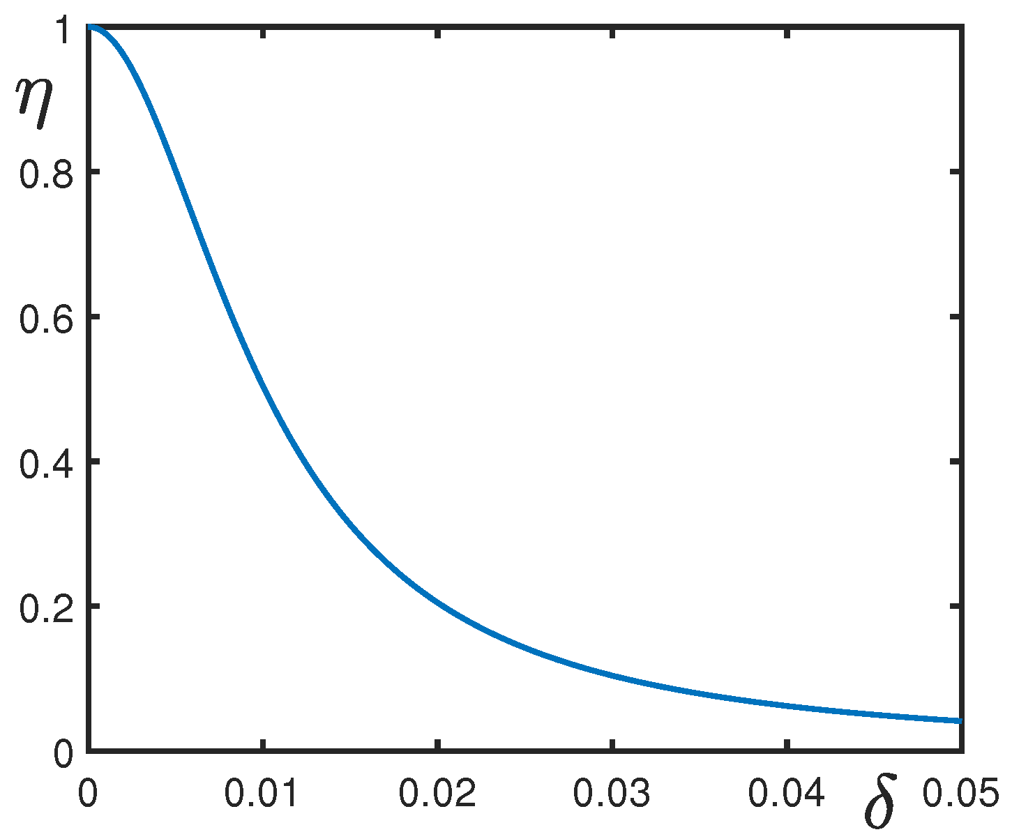
In this way, the effective order parameter can be defined as the normalized maximal coherence intensity

$$\eta \equiv \frac{w(t_0,\delta )}{w(t_0,0)}.$$

(72)

From Equation (68), we find the maximal coherence intensity

$$w(t_0,\delta )={\left(1-\frac{\gamma {\gamma }_2}{{\gamma }_0{\omega }_0}-\frac{{\gamma }_2{\omega }_0}{\gamma {\gamma }_0}{\delta }^2\right)}^2.$$

(73)

Thus, introducing the critical detuning

$${\delta }_c\equiv \sqrt{\frac{\gamma }{{\omega }_0}\left(\frac{{\gamma }_0}{{\gamma }_2}-\frac{\gamma }{{\omega }_0}\right)}$$

(74)

we obtain the order parameter

$$\eta ={\left(1-\frac{{\delta }^2}{{\delta }_c^2}\right)}^2$$

(75)

whose behavior as a function of the relative detuning $\delta$ is demonstrated in Figure 3.

It is worth noting that the non-zero transverse magnetization does not imply magnon condensation but merely means that the average magnetic moment of the system rotates around the z-axis, so that the total magnetization is not directed along this axis [40]. The correct introduction of magnons in a nonequilibrium picture requires employing the Holstein–Primakov transformation with respect to the local in time axis defined by the instantaneous time-dependent direction of the total average magnetization [41].

7. Conclusions

We have demonstrated that resonance phenomena can be treated as a kind of nonequilibrium phase transitions. Resonance phenomena, similar to equilibrium phase transitions, are accompanied by symmetry breaking and can be described by order parameters. Thus, under spin-wave resonance and helicon resonance, the magnetization inside a metallic plate, induced by an incident electromagnetic field, becomes periodic, with a slight perturbation caused by attenuation. In the case of spin-reversal resonance, spin rotation symmetry breaks, and the role of the order parameter is played by the coherence intensity. Experimental study of the behavior of the order parameters can yield information about the properties of the considered materials.

It is worth emphasizing that resonance phenomena are usually observed in finite systems. Finite-width metallic plates were considered in the case of spin-wave and helicon resonances. For the spin-reversal resonance, it was a finite sample that could be inserted in a resonator electric coil of a finite volume. Symmetry breaking in finite systems is a delicate topic, as it is quite different from the symmetry breaking in infinite systems exhibiting equilibrium phase transitions. The effects of symmetry breaking in finite quantum systems have recently been described in the review article [42]. The present paper can be considered as an additional chapter for this review.