Fermionic Properties of Two Interacting Bosons in a Two-Dimensional Harmonic Trap

1
Departament de Física Quàntica i Astrofísica, Universitat de Barcelona, Martí i Franquès 1, 08028 Barcelona, Spain
2
Institut de Ciències del Cosmos (ICCUB), Universitat de Barcelona, Martí i Franquès 1, 08028 Barcelona, Spain
3
Institut de Ciències Fotòniques, Parc Mediterrani de la Tecnologia, 08860 Barcelona, Spain
*
Author to whom correspondence should be addressed.
Condens. Matter 2018, 3(1), 9; https://doi.org/10.3390/condmat3010009
Submission received: 30 January 2018
/
Revised: 9 March 2018
/
Accepted: 12 March 2018
/
Published: 15 March 2018
(This article belongs to the Special Issue Proceedings of the conference SuperFluctuations 2017)
Abstract
:The system of two interacting bosons in a two-dimensional harmonic trap is compared with the system consisting of two noninteracting fermions in the same potential. In particular, we discuss how the properties of the ground state of the system, e.g., the different contributions to the total energy, change as we vary both the strength and range of the atom–atom interaction. In particular, we focus on the short-range and strong interacting limit of the two-boson system and compare it to the noninteracting two-fermion system by properly symmetrizing the corresponding degenerate ground state wave functions. In that limit, we show that the density profile of the two-boson system has a tendency similar to the system of two noninteracting fermions. Similarly, the correlations induced when the interaction strength is increased result in a similar pair correlation function for both systems.
1. Introduction
In one dimension, the Bose–Fermi mapping [1] theorem establishes a relation between the ground state energy and the wave function of strongly interacting bosons with those corresponding to noninteracting fermions in the same trapping potential. Both systems have the same energy, and the ground state wave function of the interacting bosonic system can be obtained by symmetrizing the noninteracting fermionic one by taking the absolute value. Several works have discussed the onset of the Tonks–Girardeau phase in one dimension [2,3,4,5,6,7,8,9,10,11,12,13,14,15,16,17,18,19].
In contrast, in two or more dimensions, the theorem does not apply because it is based on the principle, valid in one dimension, that if a particle is fixed at a point, the space becomes completely separated in two pieces [1]. Therefore, another particle cannot access the whole space without encountering the one that is fixed, which is not the case with more dimensions. In contrast, the mechanism described by Girardeau whereby the particles can avoid feeling the interaction remains a possibility. In our previous work [20], considering two, three, and four particles [21] in a two dimensional harmonic trap [2,22,23,24,25,26,27,28,29,30], we showed that interacting bosons avoid feeling the interaction by becoming correlated in such a way that the probability of two particles being at the same position vanishes [31].
In the present paper, we compare the numerical calculations for the ground state of two interacting bosons in two dimensions with a short-range interaction with the properties obtained from the analytical wave functions that describe two noninteracting bosons, two noninteracting fermions, and the corresponding symmetrized wave function. We show that some of the properties of the interacting two-boson system resemble the noninteracting fermionic ones. This work is organized in the following way. First, in Section 2, we present the considered Hamiltonian. In Section 3, we present the analytic wave functions mentioned above. In Section 4, we discuss how the ground state energy of the two-boson system changes as we vary the interaction. The corresponding effect on the density profiles and pair correlations is presented in Section 5. In Section 6, we briefly describe our numerical methods. Finally, in Section 7, we summarize the main conclusions of our work.
2. The Hamiltonian
The system of two interacting identical bosons in a two-dimensional isotropic harmonic trap is described by the Hamiltonian,
where the noninteracting part of the Hamiltonian reads
and the interaction is modeled by means of a Gaussian-shaped potential [20,29,32,33,34,35],
The interaction strength is controlled by g, while s defines the interaction range. In this work, we always consider purely repulsive interactions, . A comparison between zero-range models and the Gaussian-shape potential has been studied in [29]. In the present work, we concentrate on the dependence on both the strength g and the range s of the interaction. Notice, however, that we will not consider the regime of large scattering length, as in our case, with a purely repulsive interaction, the scattering length will be of the order of the range s [29,35]. The Hamiltonian can be split into the center-of-mass part and the relative part,
where is the center-of-mass coordinate, is the relative coordinate, m is the total mass, and is the reduced mass. Hereafter, we will use harmonic oscillator units, i.e., the length in units of and the energy in units of . The two pieces of the Hamiltonian in those units read
where we identify each part: the center-of-mass kinetic energy, , the relative kinetic energy, , the center-of-mass harmonic potential, , the relative part of the harmonic potential, , and the interaction term, , which has been properly transformed to the harmonic oscillator units.
3. Analytic Wave Functions to Compare with the Ground State
We are interested in understanding how the system changes its structure as we increase the interaction strength. In particular, we want to discern whether any fermionization takes place in the strong interaction limit, akin to the 1D case, despite the fact that the Bose–Fermi mapping theorem does not apply in 2D. To enlighten this discussion, we will compare the properties of our numerically obtained two-boson system with those of (1) the wave function of the ground state of two bosons in the noninteracting limit, which will correspond to first order perturbation theory; (2) the wave function of the ground state of two fermions in the noninteracting limit; and (3) the wave function obtained by symmetrizing the previous one by taking its absolute value. We will use polar coordinates to express the wave functions.
3.1. First-order Perturbation Theory
The ground state of two noninteracting bosons under the Hamiltonian in (1) is the nondegenerate state,
which is a state with zero angular momentum. Its energy is computed taking into account that it is an eigenfunction of the Hamiltonian in the noninteracting case, . The expectation value of the interaction term is
3.2. The Non-Interacting Two-Fermion System
For the noninteracting two-fermion system, the ground state would be two-fold degenerate, with a zero center-of-mass angular momentum, and the relative angular momentum equal to 1 or
The previous states are also eigenstates of , . The expectation value of the interaction energy in this case is
and the total energy is
Let us note that this contribution vanishes, as it should, for zero-range interactions, .
3.3. Bosonized Two-fermion System
If we symmetrize the previous wave functions by taking their absolute value, , we obtain bosonic wave functions which, as in 1D, do not allow bosons to sit at the same position. Notice that both fermionic wave functions, (9), are transformed into the same symmetric one:
which has no angular dependence. The main effect of this symmetrization is that is not an eigenfunction of , and the expectation value of the energy in the noninteracting case is . The interaction energy is the same as before, , and the expectation value of the total energy in this case is
The contribution of to the previous expectation value, , is not equally distributed between the kinetic and harmonic potential energy. Therefore, they do not fulfill the virial theorem, which is not necessary since is not an eigenfunction of . The expected values for the center-of-mass kinetic and harmonic potential energies are 1/2 each one, in agreement with the fact that the center-of-mass part of is an eigenfunction of and it therefore verifies the virial theorem, . For the kinetic energy of , we have to apply to the wave function the operator
which results in
The expectation value then is
and, for the harmonic potential relative energy,
To sum up, the total kinetic energy is , and the total harmonic potential energy is .
Let us stress that can be shown to be the best variational wave function, in the strong interacting limit, of the form
For , we recover . The set of functions are eigenfunctions of the center-of-mass part, . The relative kinetic energy is independent of the parameter a and can be shown as , which coincides with . The expected value of the relative harmonic oscillator potential energy is . The interaction energy reads
which tends to zero when only if . The total variational energy depending on a and s is
The energy minimum, in the short-range limit () and for strong interactions (), is reached when , which is precisely the case and the energy is .
4. The Interaction Effect in the Ground State Energy
4.1. The Energy Contributions
The ground state energy of the interacting two-boson system is obtained numerically following the procedure described in [20], an exact diagonalization of the Hamiltonian using the ARPACK implementation of the Lanczos algorithm. Here we supply additional information by splitting the total energy of the ground state into the kinetic, the harmonic potential, and the interaction contributions, in order to study, separately, the effect of increasing the interaction strength.
In Figure 1, we see that, in the noninteracting limit, , since the wave function of the ground state is the one given in (6), the total energy is 2, arising from two equal contributions from the kinetic and potential energy. Increasing the interaction strength slightly affects the interaction part of the energy. At the beginning, it starts to increase, but it remains mostly constant, decreases for larger interaction strengths, and becomes approximately 0. This reflects that the particles avoid feeling the interaction by building dynamical quantum correlations in the wave function, as discussed in [20]. The most relevant contribution to the energy increase for a larger interaction strength comes from the harmonic potential part. The kinetic energy remains approximately constant and equal to 1. Therefore, we can say that the two particles avoid feeling the interaction by separating one from the other. This reflects in an increase of the harmonic potential energy because they are further away from the center of the trap. This is consistent with the density profiles and pair correlation functions computed in [20] for different interaction strengths.
4.2. Exploring the Strongly Interacting Limit for a Short-range Interaction
In the strong interacting limit, in Figure 1, we see that the total energy, the kinetic energy, and the potential energy tend to values corresponding to the symmetrized wave function of Equation (12). Clearly, the way the energy is distributed for the strongly interacting two-boson system in the zero-range limit does not coincide with the noninteracting two-fermion system but with the energy decomposition provided by . In addition, the value of the ground state energy seems to tend to 2.5 energy units, which is the expected value of the energy for the variational wave function .
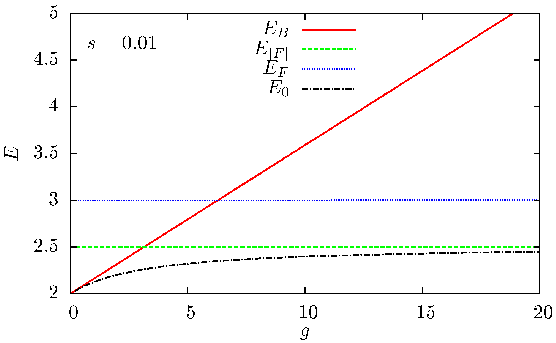
In Figure 2, we see how the ground state energy computed numerically goes from for to be very close to when g becomes large for a small fixed range, . , and depend linearly on the interaction strength g (see, respectively, Equations (8), (11), (13)). However, the slope of the lines corresponding to and in Figure 2 is positive but very small, due to the small value of s.
4.3. Exploring the Short-Range Limit for a Strong Interaction Strength
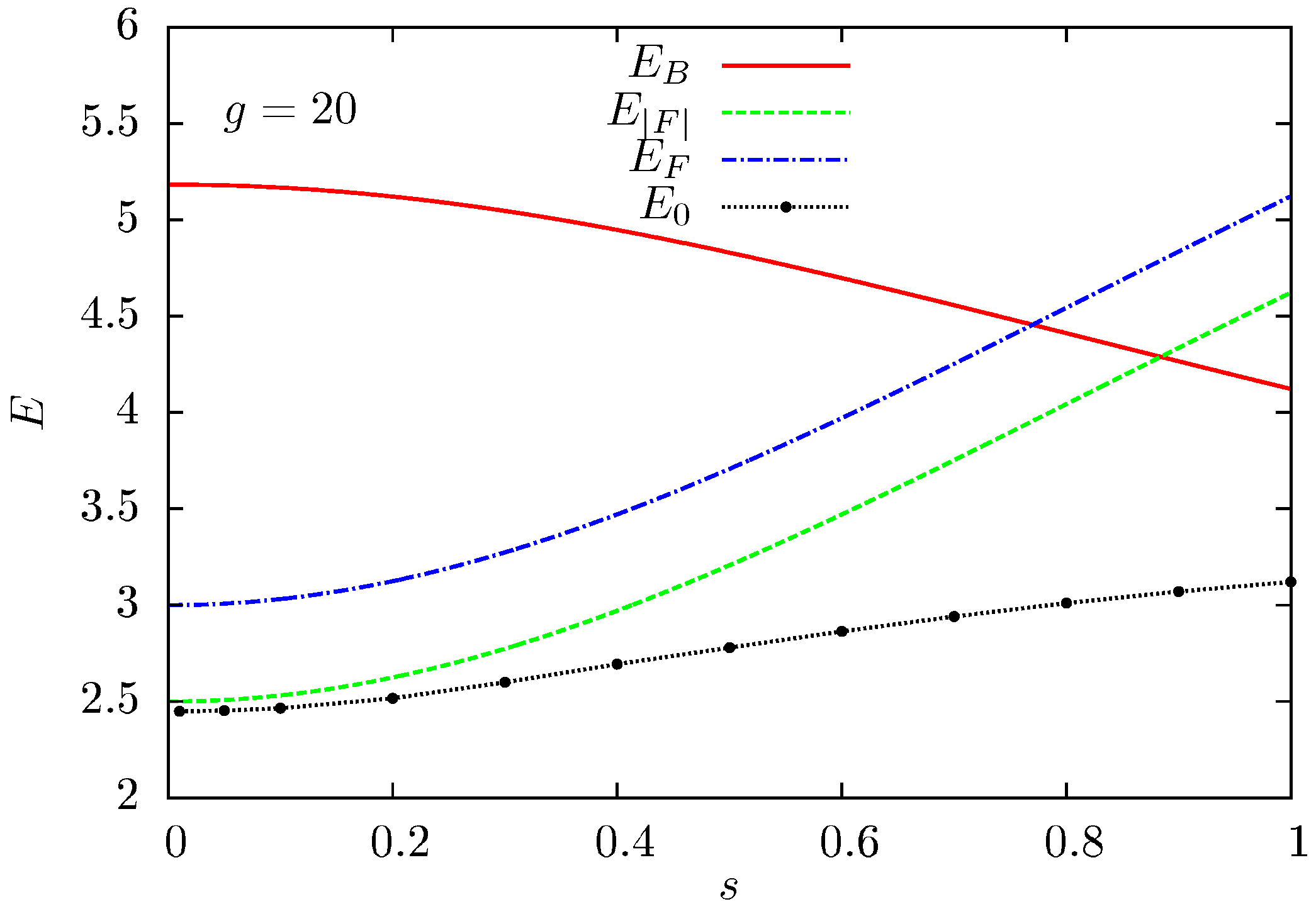
The energy dependence on the range of the interaction is shown in Figure 3, where we compare the ground state energy of the interacting two-boson system computed numerically with the expected values given by our analytic wave functions. For a fixed and strong interaction strength, , reducing the range of the interaction results in a decrease of the ground state energy of the system. The same kind of behavior is observed for and its symmetrized wave function, , since their dependence on the interaction is the same and the shift in energy between them is due to the noninteracting part of the Hamiltonian. In the short-range limit, their interaction energy tends to zero, and approaches . Differently, the interaction energy of does not vanish in the zero-range limit. In fact, the energy for this wave function increases for decreasing s.
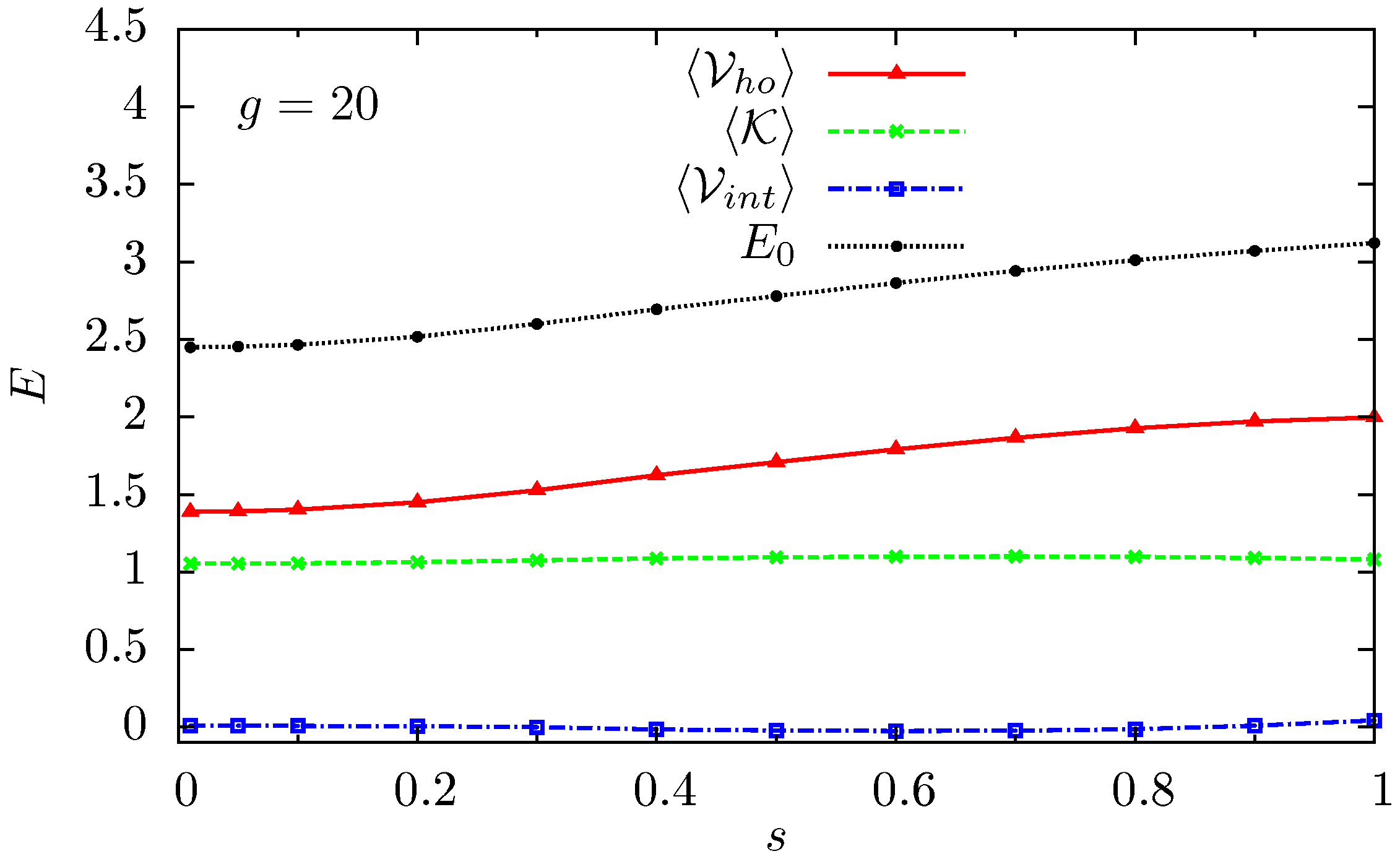
In Figure 4, we observe that not only is very close to when , but the way the energy is distributed also coincides; i.e., the expected values of the kinetic energy, the interaction energy, and the harmonic potential energy for a strong interaction in the short-range limit for the ground state of the interacting two-boson system tend to values computed for .
In addition, we show that the most relevant contributions to the energy when the range s varies comes from the harmonic potential energy, because the kinetic and interaction parts are mainly independent of s and remain constant in Figure 4.
5. The Density Profile and the Two-body Correlations
In this section, we will compare the density profile and the pair correlation function of the ground state of the trapped two boson system, with and without interactions, with the ones provided by and .
The density operator, acting on a system of N particles, is defined as
and the pair correlation operator reads
where both operators are normalized to unity. Since we consider the case of two identical particles, we compute the density profile and the pair correlation function for a given state , respectively, as follows: , and .
Using Cartesian coordinates, the wave functions of Section 3 read
The corresponding density profiles and pair correlations read
Note that both the fermionic and bosonized wave functions give the same density and pair correlation as .
From the pair correlation function and the density profile, we compute the probability of finding a particle at a distance once we have found the other at the origin, that is,
which for the two previous discussed cases is, respectively, , and .
In Figure 5a, we compare the density profiles obtained numerically for the ground state of trapped interacting two-boson system with the density profile corresponding to the noninteracting case and to the noninteracting two-fermion system. We show that, given an interaction range, there is an interaction strength such that the density profile of the interacting two-boson system is very well approximated by the two-fermion density profile. The smaller the interaction range, s, is, in which the density profiles coincide, the greater the interaction strength, g, will be. Therefore, in the short-range limit and for strong interactions, the density profile of two interacting bosons tends toward the noninteracting two-fermion profile.
In the case of the probability of finding a particle in space once we have found the other at the origin, we observe, in Figure 5b, that the numerically computed ones for the interacting two-boson system resemble the corresponding two noninteracting fermions. However, in this case, the maximum peak does not coincide, and it is closer to the center of the trap for two noninteracting fermions. The probability of finding the two bosons at the same position, i.e., at , tends toward zero when the interaction range vanishes and the interaction strength increases, as expected.
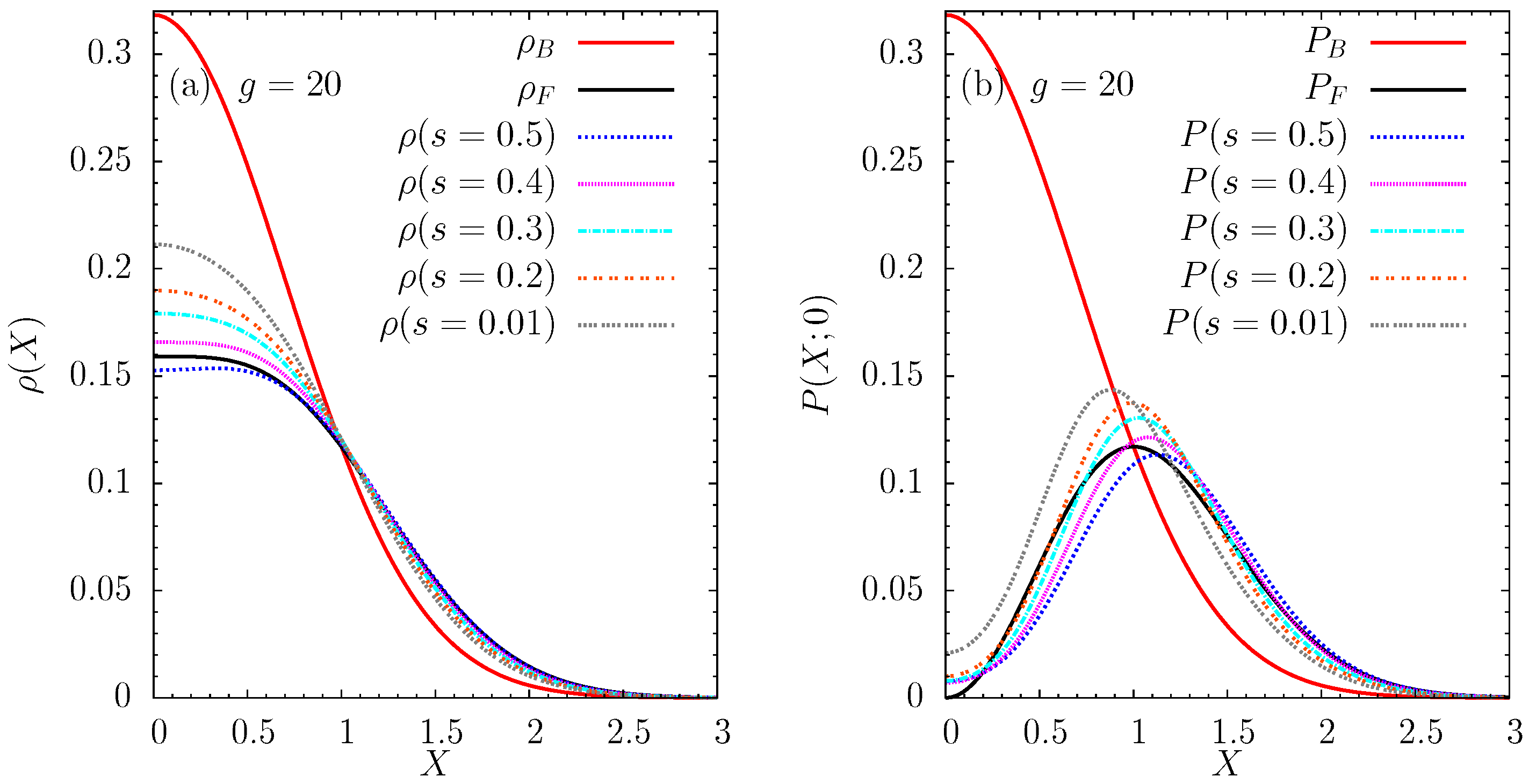
The effect of decreasing the interaction range for a fixed interaction strength is shown in Figure 6. Regarding the density profile, in panel (a), the interaction strength is strong enough in all cases so that they are closer to than to . The density peak increases for a smaller range, although there is practically no effect in the density profile for , and all of the numerical profiles fit well with . In Figure 6b, we observe that the effect of decreasing the range is such that the maximum in the probability approaches the center of the trap and the maximum value increases. However, in any case the probability vanishes at , as it does for , which would happen for greater g values and in the short-range limit, as shown in Figure 5b.
6. Numerical Method
The numerical method was previously developed by the authors and is described in detail in [20]. First, we write the many-body Hamiltonian in a second quantized form. Then we define the set of single particle states, which are taken to be the lowest energy eigenstates of the single particle Hamiltonian. Once we fix the number of particles, we can define the corresponding Fock basis for the problem. The final results should be independent of the number of single particle states. In the numerical results reported in this paper, we have used up to 200 single particle states. The resulting Hamiltonian is then diagonalized using the ARPACK implementation of the Lanczos algorithm in order to compute the low-energy spectrum of the system and, in particular, the ground state.
7. Conclusions
In two dimensions, the ground state energy of two strongly interacting bosons in a harmonic trap for a short-range interaction is not equal to the noninteracting two-fermion system in the same potential, as it was in one dimension. However, the wave function resulting from symmetrizing the corresponding noninteracting fermionic ground state is found to be a very good variational trial wave function. It provides an upper-bound very close to the ground state energy obtained by exact diagonalization in the strong interacting and short-range limit. Even more, the distribution of the energy between the kinetic and harmonic potential parts in that limit also coincides. The increase of the energy with the interaction strength comes, mostly, from the harmonic potential contribution to the energy since the kinetic energy remains almost constant and the interaction energy approximately zero. The bosons avoid feeling the interaction by being more separate and, therefore, further from the center of the trap, which is also reflected in the density profiles obtained. The correlations induced by the interaction cause the density profile of the strongly interacting bosons to tend toward the noninteracting two-fermion profile. For the pair correlation function, we have found qualitatively the same kind of behavior.
Acknowledgments
The authors thank S. Pilati for his comments and discussions about the scattering length and the regularized pseudopotential in two dimensions. The authors acknowledge financial support of grants 2014SGR-401 from Generalitat de Catalunya and FIS2014-54672-P from the MINECO (Spain). P.M. was supported by an FI grant from Generalitat de Catalunya.
Author Contributions
Main ideas were conceived by Pere Mujal, Artur Polls, and Bruno Julia-Diaz. Pere Mujal and Artur Polls performed all the calculations. Pere Mujal wrote a first version of the manuscript. Pere Mujal, Artur Polls and Bruno Julia-Diaz discussed the results and wrote the final version of the manuscript.
Conflicts of Interest
The authors declare no conflict of interest.
References
- Girardeau, M. Relationship between systems of impenetrable bosons and fermions in one dimension. J. Math. Phys. 1960, 1, 516. [Google Scholar] [CrossRef]
- Busch, T.; Englert, B.G.; Rzazewski, K.; Wilkens, M. Two cold atoms in a harmonic trap. Found. Phys. 1998, 28, 549. [Google Scholar] [CrossRef]
- Girardeau, M.D.; Wright, E.M.; Triscari, J.M. Ground-state properties of a one-dimensional system of hard-core bosons in a harmonic trap. Phys. Rev. A 2001, 63, 033601. [Google Scholar] [CrossRef]
- Paredes, B.; Widera, A.; Murg, V.; Mandel, O.; Fölling, S.; Cirac, I.; Shlyapnikov, G.V.; Hänsch, T.W.; Bloch, I. Tonks-Girardeau gas of ultracold atoms in an optical lattice. Nature 2004, 429, 277. [Google Scholar] [CrossRef] [PubMed]
- Kinoshita, T.; Wenger, T.; Weiss, D.S. Observation of a one-dimensional Tonks-Girardeau Gas. Science 2004, 305, 1125. [Google Scholar] [CrossRef] [PubMed]
- Pupillo, G.; Rey, A.M.; Williams, C.J.; Clark, C.W. Extended fermionization of 1D bosons in optical lattices. New J. Phys. 2006, 8, 161. [Google Scholar] [CrossRef]
- Tempfli, E.; Zöllner, S.; Schmelcher, P. Excitations of attractive 1d bosons: Binding versus fermionization. New J. Phys. 2008, 10, 103021. [Google Scholar] [CrossRef]
- Bakr, W.S.; Peng, A.; Tai, M.E.; Ma, R.; Simon, J.; Gillen, J.I.; Fölling, S.; Pollet, L.; Greiner, M. Probing the superfluid-to-Mott insulator transition at the single-atom level. Science 2010, 329, 547. [Google Scholar] [CrossRef] [PubMed] [Green Version]
- Sherson, J.F.; Weitenberg, C.; Endres, M.; Cheneau, M.; Bloch, I.; Khur, S. Single-atom-resolved fluorescence imaging of an atomic Mott insulator. Nature 2010, 467, 68. [Google Scholar] [CrossRef] [PubMed]
- Deuretzbacher, F.; Cremon, J.C.; Reimann, S.M. Ground-state properties of few dipolar bosons in a quasi-one-dimensional harmonic trap. Phys. Rev. A 2010, 81, 063616. [Google Scholar] [CrossRef]
- Kościk, P. Quantum correlations of a few bosons within a harmonic trap. Few-Body Syst. 2012, 52, 49. [Google Scholar] [CrossRef]
- Brouzos, I.; Schmelcher, P. Construction of analytical many-body wave functions for correlated bosons in a harmonic trap. Phys. Rev. Lett. 2012, 108, 045301. [Google Scholar] [CrossRef] [PubMed]
- García-March, M.A.; Juliá-Díaz, B.; Astrakharchik, G.E.; Busch, Th.; Boronat, J.; Polls, A. Sharp crossover from composite fermionization to phase separation in microscopic mixtures of ultracold bosons. Phys. Rev. A 2013, 88, 063604. [Google Scholar] [CrossRef]
- García-March, M.A.; Juliá-Díaz, B.; Astrakharchik, G.E.; Boronat, J.; Polls, A. Distinguishability, degeneracy, and correlations in three harmonically trapped bosons in one dimension. Phys. Rev. A 2014, 90, 063605. [Google Scholar] [CrossRef]
- Wilson, B.; Foerster, A.; Kuhn, C.C.N.; Roditi, I.; Rubeni, D. A geometric wave function for a few interacting bosons in a harmonic trap. Phys. Lett. A 2014, 378, 1065. [Google Scholar] [CrossRef]
- García-March, M.A.; Juliá-Díaz, B.; Astrakharchik, G.E.; Busch, Th.; Boronat, J.; Polls, A. Quantum correlations and spatial localization in one-dimensional ultracold bosonic mixtures. New J. Phys. 2014, 16, 103004. [Google Scholar] [CrossRef]
- Barfknecht, R.E.; Dehkharghani, A.S.; Foerster, A.; Zinner, N.T. Correlation properties of a three-body bosonic mixture in a harmonic trap. J. Phys. B At. Mol. Opt. Phys. 2016, 49, 135301. [Google Scholar] [CrossRef]
- Pyzh, M.; Krönke, S.; Weitenberg, C.; Schmelcher, P. Spectral properties and breathing dynamics of a few-body Bose-Bose mixture in a 1d harmonic trap. arXiv, 2017; arXiv:1707.03758. [Google Scholar]
- Kościk, P.; Sowiński, T. Exactly solvable model of two trapped quantum particles interacting via finite-range soft-core interactions. Sci. Rep. 2018, 8, 48. [Google Scholar] [CrossRef] [PubMed]
- Mujal, P.; Sarlé, E.; Polls, A.; Juliá-Díaz, B. Quantum correlations and degeneracy of identical bosons in a two-dimensional harmonic trap. Phys. Rev. A 2017, 96, 043614. [Google Scholar] [CrossRef]
- Blume, D. Few-body physics with ultracold atomic and molecular systems in traps. Rep. Prog. Phys. 2012, 75, 046401. [Google Scholar] [CrossRef] [PubMed]
- Kartavtsev, O.I.; Malykh, A.V. Universal low-energy properties of three two-dimensional bosons. Phys. Rev. A 2006, 74, 042506. [Google Scholar] [CrossRef]
- Christensson, J.; Forssén, C.; Åberg, S.; Reimann, S.M. Effective-interaction approach to the many-boson problem. Phys. Rev. A 2009, 79, 012707. [Google Scholar] [CrossRef]
- Shea, P.; van Zyl, B.P.; Bhaduri, R.K. The two-body problem of ultra-cold atoms in a harmonic trap. Am. J. Phys. 2009, 77, 511. [Google Scholar] [CrossRef]
- Liu, X.J.; Hu, H.; Drummond, P.D. Exact few-body results for strongly correlated quantum gases in two dimensions. Phys. Rev. B 2010, 82, 054524. [Google Scholar] [CrossRef]
- Farrell, A.; van Zyl, B.P. Universality of the energy spectrum for two interacting harmonically trapped ultra-cold atoms in one and two dimensions. J. Phys. A Math. Theor. 2010, 43, 015302. [Google Scholar] [CrossRef]
- Zinner, N.T. Universal two-body spectra of ultracold harmonically trapped atoms in two and three dimensions. J. Phys. A Math. Theor. 2012, 45, 205302. [Google Scholar] [CrossRef]
- Daily, K.M.; Yin, X.Y.; Blume, D. Occupation numbers of the harmonically trapped few-boson system. Phys. Rev. A 2012, 85, 053614. [Google Scholar] [CrossRef]
- Doganov, R.A.; Klaiman, S.; Alon, O.E.; Streltsov, A.I.; Cederbaum, L.S. Two trapped particles interacting by a finite-range two-body potential in two spatial dimensions. Phys. Rev. A 2013, 87, 033631. [Google Scholar] [CrossRef]
- Whitehead, T.M.; Schonenberg, L.M.; Kongsuwan, N.; Needs, R.J.; Conduit, G.J. Pseudopotential for the two-dimensional contact interaction. Phys. Rev. A 2016, 93, 042702. [Google Scholar] [CrossRef]
- Romanovsky, I.; Yannouleas, C.; Landman, U. Cristalline boson phases in harmonic traps: Beyond the Gross-Pitaevskii mean field. Phys. Rev. Lett. 2004, 93, 230405. [Google Scholar] [CrossRef] [PubMed]
- Klaiman, S.; Lode, A.U.J.; Streltsov, A.I.; Cederbaum, L.S.; Alon, O.E. Breaking the resilience of a two-dimensional Bose-Einstein condensate to fragmentation. Phys. Rev. A 2014, 90, 043620. [Google Scholar] [CrossRef]
- Katsimiga, G.C.; Mistakidis, S.I.; Koutentakis, G.M.; Kevrekidis, P.G.; Schmelcher, P. Many-body quantum dynamics in the decay of bent dark solitons of Bose-Einstein condensates. New J. Phys. 2017, 19, 123012. [Google Scholar] [CrossRef]
- Bolsinger, V.J.; Krönke, S.; Schmelcher, P. Beyond mean-field dynamics of ultra-cold bosonic atoms in higher dimensions: Facing the challenges with a multi-configurational approach. J. Phys. B At. Mol. Opt. Phys. 2017, 50, 034003. [Google Scholar] [CrossRef]
- Jeszenski, P.; Cherny, A.Y.; Brand, J. The s-wave scattering length of a Gaussian potential. arXiv, 2018; arXiv:1802.07063. [Google Scholar]
Figure 1.
Ground state energy of two interacting bosons in a two-dimensional harmonic trap, , depending on the interaction strength, g, for a fixed and small interaction range, s. We present the harmonic potential part, , the kinetic part, , and the interaction part, . The energies were computed numerically using the first single-particle eigenstates of the harmonic oscillator (see Section 6 for details).
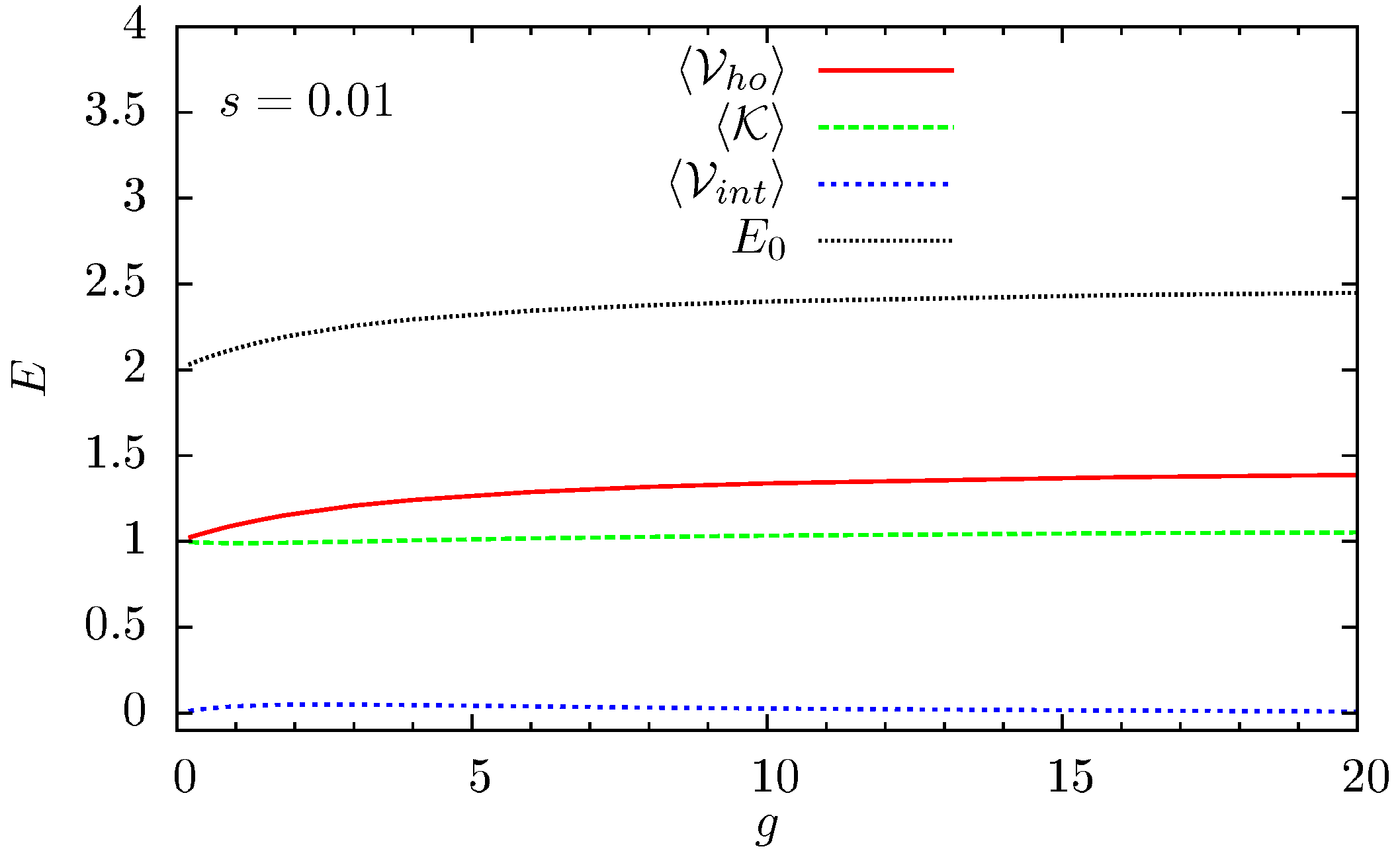
Figure 2.
Ground state energy of two interacting bosons in a harmonic trap, , as in Figure 1, depending on the interaction strength, g, and for a fixed range, s. The exact calculation is compared with the expectation value of the energy of the wave functions of two noninteracting bosons, , two noninteracting fermions, , and the corresponding symmetrized wavefunction, , which are given, respectively, by Equations (8), (11), and (13).

Figure 3.
Ground state energy of two interacting bosons in a harmonic trap, , depending on the interaction range, s, and for a fixed interaction strength, g. The numerical result is compared with the expectation value of the energy of the wave functions of two noninteracting bosons, , two noninteracting fermions, , and its the symmetrized wavefunction, , which are given, respectively, by Equations (8), (11), and (13).

Figure 4.
Ground state energy of two interacting bosons in a harmonic trap, , depending on the interaction range, s, for a fixed interaction strength, g. We also show the different contributions, , , and . The energies were computed numerically using the first single-particle eigenstates of the harmonic oscillator (see Section 6 for details).

Figure 5.
(a) Density profiles of two noniteracting bosons, , two noninteracting fermions, , and three numerically computed profiles for different ranges and interaction strength for the interacting two-boson system; (b) Probability of finding a particle at a distance X from the origin once a particle is found at in the same cases. For the numerical calculations, the number of single-particle eigenstates of the harmonic oscillator used was (see Section 6 for details).
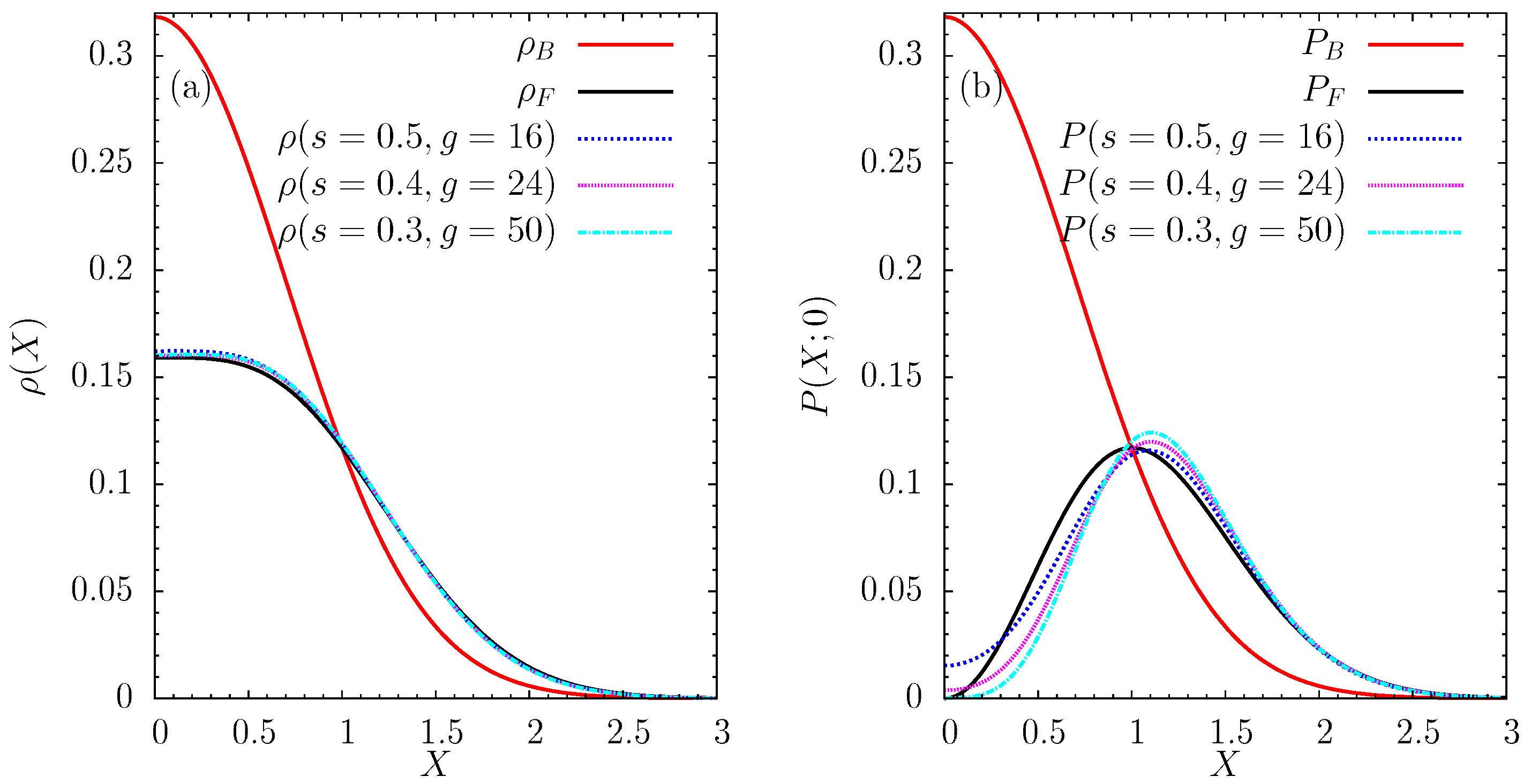
Figure 6.
(a) Density profiles of two noniteracting bosons, , two noninteracting fermions, , and four numerically computed profiles for different ranges fixing the interaction strength for the interacting two-boson system; (b) Probability of finding a particle at a distance X from the origin once a particle is found at in the same cases. For the numerical calculations the number of single-particle eigenstates of the harmonic oscillator used was (see Section 6 for details).
© 2018 by the authors. Licensee MDPI, Basel, Switzerland. This article is an open access article distributed under the terms and conditions of the Creative Commons Attribution (CC BY) license (http://creativecommons.org/licenses/by/4.0/).
Share and Cite
MDPI and ACS Style
Mujal, P.; Polls, A.; Juliá-Díaz, B. Fermionic Properties of Two Interacting Bosons in a Two-Dimensional Harmonic Trap. Condens. Matter 2018, 3, 9. https://doi.org/10.3390/condmat3010009
AMA Style
Mujal P, Polls A, Juliá-Díaz B. Fermionic Properties of Two Interacting Bosons in a Two-Dimensional Harmonic Trap. Condensed Matter. 2018; 3(1):9. https://doi.org/10.3390/condmat3010009
Chicago/Turabian StyleMujal, Pere, Artur Polls, and Bruno Juliá-Díaz. 2018. "Fermionic Properties of Two Interacting Bosons in a Two-Dimensional Harmonic Trap" Condensed Matter 3, no. 1: 9. https://doi.org/10.3390/condmat3010009