Scintillator Pixel Detectors for Measurement of Compton Scattering

Abstract

The Compton scattering of gamma rays is commonly detected using two detector layers, the first for detection of the recoil electron and the second for the scattered gamma. We have assembled detector modules consisting of scintillation pixels, which are able to detect and reconstruct the Compton scattering of gammas with only one readout layer. This substantially reduces the number of electronic channels and opens the possibility to construct cost-efficient Compton scattering detectors for various applications such as medical imaging, environment monitoring, or fundamental research. A module consists of a 4 × 4 matrix of lutetium fine silicate scintillators and is read out by a matching silicon photomultiplier array. Two modules have been tested with a ${}^{22}$Na source in coincidence mode, and the performance in the detection of 511 keV gamma Compton scattering has been evaluated. The results show that Compton events can be clearly distinguished with a mean energy resolution of 12.2% ± 0.7% in a module and a coincidence time resolution of $0.56\pm 0.02$ ns between the two modules.

1. Introduction

Compton scattering is a well-known process in which an incoming gamma ray is interacting with an electron, leaving a scattered gamma and a recoil electron in the final state. To detect and to reconstruct the Compton scattering fully, one needs position- and energy-sensitive detectors. The interaction point is determined from the location where the recoil electron is absorbed, while the direction of the scattered gamma is determined from its energy and the position of the absorption relative to the impact point.

The Compton scattering of gamma rays has lately received a growing interest in developing medical physics applications such as the new generation of Positron Emission Tomography (PET) devices, where several studies have shown that it has the potential to improve PET image quality, since it provides information about the gamma ray polarization, as an additional handle to improve the signal to noise ratio [1,2,3].

A common method of detection and reconstruction of gamma Compton scattering is to use two detector layers, the first for measurement of energy and the location of the recoil electron and the second for measuring the energy and absorption location of the scattered gamma, e.g., [4,5,6,7,8]. In PET, however, detectors are highly segmented and have a large coverage, as a pre-requisite to achieve a good spatial resolution and sensitivity; therefore, two highly-granular detector layers for Compton measurements would dramatically increase the cost of the apparatus. Several developments optimized for astrophysics observations use single detector layers to measure gamma ray polarization via Compton scattering [9,10], but a single-layer system PET system exploiting the gamma polarization has not been experimentally realized.

We assembled single-layer Compton detectors, and a system of two such modules was set up, as described in [11]. Each module consists of a 4 × 4 scintillator pixel array, read out on the back side by a matching array of Silicon Photomultipliers (SiPM) in a one-to-one coupling scheme. In this paper, we will show that such detectors are able to reconstruct the Compton scattering events of 511 keV gamma rays fully, as a prerequisite for gamma polarization measurements. The details of the energy, angle, and time reconstruction methods are presented in Section 2, and the detector performance is presented in Section 3.

2. Materials and Methods

2.1. Experimental Setup

A system of two detector modules labeled A and B has been set up. Each module consists of a 4 × 4 array of Lutetium Fine Silicate (LFS) scintillator pixels produced by Zecotec Inc. (Figure 1), read out by a matching array of SiPM produced by Hamamatsu (Model S13361-3050AE-04). Signals from each channel are first amplified, then digitized by fast pulse digitizers (CAEN V1743) at 1.6 GS/s and stored for offline analysis. A detailed description of the experimental setup and the detector performance is given in [11]. In the setup presented in this work, we additionally applied silicon grease as the optical coupling medium between the scintillators and the SiPMs (see SubSection 2.2 for details).

A ${}^{22}\mathrm{Na}$ positron source (activity $\approx 1\mu \mathrm{Ci}$) in an aluminum case was positioned between the modules, 4 cm from the front face of each detector, providing two coincident annihilation gammas of 511 keV. The data acquisition system triggered only on events where a coincident detection occurred in both modules. The coincidence condition efficiently suppressed the random background from ${}^{176}\mathrm{Lu}$ decays intrinsic to the scintillation material. The measurements were performed at room temperature typically in a range from 20–22 ${}^{\circ }$C and at a moderate bias voltage $U_b=U_{br}+1.6$ V, $U_{br}$ being the SiPM breakdown voltage.

2.2. Scintillator-SiPM Optical Coupling

In the setup presented in this work, silicon optical grease (BC-630 by Saint-Gobain) was used as the optical coupling material between the scintillator crystals and the SiPM arrays. This resulted in an increased light propagation from crystals to SiPMs, observed as an increase of signal amplitudes up to 40%, under the same operating conditions and reflected in an improvement of the energy resolution from $\Delta E/E=12.9\%$ down to $\Delta E/E=11.4\%$. However, this was not the case for all pixels: we found that after applying the silicon grease, some amplitudes remained at the same level as before. Consequently, small variations of energy resolution from pixel-to-pixel have been observed, resulting in the mean energy resolution of a module of 12.2% ± 0.7% (at 511 keV). Different optical coupling methods will be investigated in the future to provide a more uniform detector performance.

2.3. Signal Processing

Signals from all scintillator channels in triggered events are stored, which enables offline optimization of processing algorithms for specific applications. In our approach, the energy deposition was reconstructed by signal integration and the arrival time from the signal leading edge.

For energy reconstruction, three quantities are extracted: the average baseline, the signal amplitude, and the signal integral. The baseline is determined as the average of at least 20 samples before the signal rising edge; the amplitude is determined as the difference of the maximum sample amplitude and the baseline; and the integral is determined by summing the sampled voltages (after baseline subtraction) in the region where the signals are non-zero. An example is in Figure 2a.

To reconstruct the time of the signal arrival, we use the leading edge method: a fixed threshold is set as close to the baseline as possible to enable triggering on the very first scintillation photons, as discussed in [12]. In the presented results, the threshold is −15 mV (typical signal amplitudes reach several hundreds of mV). The algorithm searches for the sample that is just above the threshold, S, then uses linear interpolation between samples S and $S-1$ to estimate the time when the threshold had been crossed, which is taken as the time of signal arrival (Figure 2b).

2.4. Energy Reconstruction

2.4.1. Energy Calibration

The raw energy spectrum is obtained as the spectrum of signal integrals for each pixel. It is first corrected for non-linearity, which is present due to the finite number of micro cells per SiPM, as described in [11]. Then, it is calibrated by fitting a Gaussian to the annihilation peak and setting the corresponding value to 511 keV. For the second calibration point, we assume the zero in the integral spectrum corresponds to zero energy, inherent to the signal processing algorithm, which subtracts the baseline on an event-by-event basis. The calibration is performed for each data acquisition run, typically lasting two hours. In this time window, the temperature variations are <0.1 ${}^{\circ }$C and therefore have a small influence on the calibration parameters (<0.5%), which is considered negligible compared to the mean energy resolution (12.2% ± 0.7% at 511 keV).

2.4.2. Light Sharing Correction

An energy correlation between the adjacent crystal pixels had been observed, as reported in [11]. When a significantly large signal is observed in a pixel, small signals are observed in adjacent pixels, with amplitudes proportional to the main signal amplitude, as demonstrated in Figure 3. This can be attributed to light sharing, either as light leaking through crystal sides and the Teflon reflector (0.06 mm thick) between the pixels or by light leaking at the contact with the SiPM array. When single pixel events are considered, the light sharing does not cause an energy reconstruction problem, since the energy calibration is performed using single pixel spectra. However, in two-pixel events where two adjacent pixels fire, the light sharing disguises the original energy deposition in the pixels and must be corrected for. In order to reconstruct the Compton scattering angle $\theta$ (see Section 2.5.1) correctly, it is important to determine the true energy response of the pixels. We present a method to decouple the observed energies and obtain real energy depositions in the pixels.

The energy contribution in a pixel coming form an adjacent neighbor can be described as $E_{Adj.neighbor}=ϵE_{main}$. Suppose two adjacent pixels are labeled 1 and 2. The measured energy responses are:

$$\begin{array}{c}\hfill E_1=E_1^o+{ϵ}_{12}{E}_2^o\end{array}$$

(1)

$$\begin{array}{c}\hfill E_2=E_2^o+{ϵ}_{12}{E}_1^o\end{array}$$

(2)

where $E_1^o$ and $E_2^o$ are the original energy depositions in the pixels and ${ϵ}_{12}$ is the sharing fraction characteristic of that pixel pair. It follows that:

$$E_1+E_2=(E_1^o+E_2^o)(1+{ϵ}_{12})$$

(3)

with:

$$E_1^o+E_2^o=E_{\gamma }$$

(4)

being the gamma particle energy. Hence, the energy sum of adjacent pixels 1 and 2 is boosted by a factor $(1+{ϵ}_{12})$. This is observed in Figure 4a. By combining Equation (1) to Equation (4), one obtains the original deposited energies as:

$$\begin{array}{c}\hfill E_1^o=\frac{E_1-{ϵ}_{12}{E}_2}{1-{ϵ}_{12}^2}\end{array}$$

(5)

$$\begin{array}{c}\hfill E_2^o=\frac{E_2-{ϵ}_{12}{E}_1}{1-{ϵ}_{12}^2}\end{array}$$

(6)

Since variations of ${ϵ}_{12}$ are relatively small, we replace it by average module values $<{ϵ}_A>=0.060$ for detector module A and $<{ϵ}_B>=0.066$ for module B.

When two fired pixels are not adjacent neighbors, the shift of the summed energy is much smaller, as summarized in

Table 1. The mean fraction of neighbor-to-main pixel energy response, $<ϵ>$, for the three most abundant event topologies in modules A and B, respectively.

Neighbors	Pixel Distance d (mm)	<${\mathit{ϵ}}_{\mathit{A}}$>	<${\mathit{ϵ}}_{\mathit{B}}$>
1st adjacent	3.2	0.060	0.066
1st diagonal	4.5	0.020	0.019
2nd direct	6.4	0.013	0.014

. This is also visible in Figure 4a. It can be due to indirect light sharing through an intermediate pixel or even due to dark counts from the SiPMs, which are double counted in the sum when two pixels fire. Since the effect is much smaller than with the adjacent neighbors, it is simply corrected for by scaling the measured pixel energy, E, by the same fraction:

$$E^o=(1-ϵ)E$$

(7)

After applying these corrections, the energy sum $E_1^o+E_2^o$ is correctly reconstructed at 511 keV, as shown in Figure 4b.

2.5. Reconstruction of Compton Scattering Angles

The Compton events are selected by requiring two fired pixels in a module, with the sum of pixel energies, $E_1^o+E_2^o$ within $\pm 3\sigma$ of the full energy peak at 511 keV ($435\mathrm{keV}<E_1^o+E_2^o<590\mathrm{keV}$) and the energy of any pixel $60\mathrm{keV}<E_{px}^o<405\mathrm{keV}$. In the latter condition, the lower bound of 60 keV is set conservatively to avoid possible noise contributions, and the upper bound of 405 keV is determined by the Compton edge (340 keV $\pm 3\sigma$).

In Compton scattering, the scattering angle $\theta$ is defined as the angle between the momenta vectors of the incoming and the scattered gamma $(\overrightarrow{k_0},\overrightarrow{k^{\prime }})$. The scattering angle $\theta$ does not uniquely characterize the direction of the scattered gamma; it only defines a cone on which the scattered momentum lies. Therefore, to reconstruct the momentum vector of the scattered gamma fully, one needs to determine the angle $\varphi$ (sometimes denoted as the azimuthal angle). In our case, it is defined as the angle between the scattering plane $(\overrightarrow{k_0},\overrightarrow{k^{\prime }})$ and the horizontal plane $(\widehat{x},\widehat{z})$.

2.5.1. Scattering Angle $\theta$

In Compton scattering, the scattering angle $\theta$ is related to the energy of the scattered gamma by kinematics:

$$\theta =\mathrm{acos}\left(m_e{c}^2\left(\frac{1}{E_{\gamma }}-\frac{1}{E_{\gamma }^{{}^{\prime }}}\right)-1\right)$$

(8)

However, one needs to determine which of the two fired pixels’ energies corresponds to the recoil electron energy, $E_e^{{}^{\prime }}$, and which to the scattered photon energy, $E_{\gamma }^{{}^{\prime }}$. Specifically for $E_{\gamma }=511$ keV and $\theta <{60}^{\circ }$, this is uniquely determined, since in this case, $E_e^{{}^{\prime }}<E_{\gamma }^{{}^{\prime }}$. For $\theta >{60}^{\circ }$, corresponding to pixel energies $171\mathrm{keV}<E_{px}^o<340\mathrm{keV}$, the scattering angle determination is ambiguous, as it is not possible to directly discriminate between the forward and backward scattering, unless the detector provides depth-of-interaction information; e.g., for $\theta ={70}^{\circ }$, one expects the fired pixels with energies $E_e^{{}^{\prime }}=203$ keV and $E_{\gamma }^{{}^{\prime }}=308$ keV. However, scattering at $\theta ={121}^{\circ }$ would result in the same pixel energies, $E_e^{{}^{\prime }}=308$ keV and $E_{\gamma }^{{}^{\prime }}=203$ keV. According to Klein–Nishina relation, the ratio of the differential cross-sections for scattering at these angles is ${\eta }_{f/b}=\frac{d\sigma }{d\mathsf{\Omega }}{{|}_{\theta ={70}^{\circ }}/\frac{d\sigma }{d\mathsf{\Omega }}|}_{\theta ={121}^{\circ }}=1.46$, meaning that the forward scattering is more probable.

The forward-backward ambiguity can be further suppressed by exploiting the detector design (i.e., segmentation and material). The backward scattered gammas have lower energy than the forward scattered ones, so they will have a shorter attenuation length. Let the distance traveled by a scattered gamma be $D=d/\sin \theta$, where d is the pixel distance in the x-y plane. The ratio of the forward to backward scattered gammas is then:

$${\xi }_{f/b}=e^{\frac{-D\left({\theta }_f\right)}{\mu \left(E_f\right)}}/e^{\frac{-D\left({\theta }_b\right)}{\mu \left(E_b\right)}}$$

(9)

where $\mu \left(E\right)$ is the attenuation length in the material for given energy E and $D\left({\theta }_f\right)$ and $D\left({\theta }_b\right)$ are the pathlengths for forward and backward scattering, respectively. The ratio of the probabilities to observe forward versus backward scattering is $P_f/P_b={\eta }_{f/b}\times {\xi }_{f/b}$.

Table 2. Estimated ratio of forward to backward scattering probabilities for two angle combinations $\theta$ with ambiguous energy response. Attenuation lengths in the Lutetium Fine Silicate (LFS) scintillator derived from [13].

${\mathit{\theta }}_{\mathit{f}}/{\mathit{\theta }}_{\mathit{b}}$	${\mathit{\eta }}_{\mathit{f}/\mathit{b}}$	Pixel Distance d (mm)	${\mathit{\xi }}_{\mathit{f}/\mathit{b}}$	${\mathit{P}}_{\mathit{f}}/{\mathit{P}}_{\mathit{b}}$
${80}^{\circ }$/${102}^{\circ }$	1.20	3.2 (1st neighbors)	1.4	1.7
		6.4 (2nd neighbors)	1.9	2.3
${70}^{\circ }$/${121}^{\circ }$	1.46	3.2 (1st neighbors)	2.5	3.6
		6.4 (2nd neighbors)	6.1	8.9

gives an example for two angles in the region of interest ($\theta >{60}^{\circ }$).

In our approach, the scattering angle $\theta$ is reconstructed assuming the forward scattering, meaning the pixel with the higher energy ($E_{high}$) is associated with the scattered gamma, while the pixel with the lower energy ($E_{low}$) is associated with the recoil electron. For 511 keV gammas, this is always the case for $\theta <{60}^{\circ }$, but it is also justified to assume so for larger angles since the probability to observe the forward scattering is always larger than the one to observe the backward scattering, $P_f/P_b>1$.

The uncertainty in the determination of the scattering angle is dominated by the energy resolution of the pixels. After substituting $E_{\gamma }=E_{e^{\prime }}+E_{{\gamma }^{\prime }}$ in Equation (8), it follows:

$${\sigma }_{\theta }^2={\left(\frac{\partial \theta }{\partial E_{e^{\prime }}}{\sigma }_{E_{e^{\prime }}}\right)}^2+{\left(\frac{\partial \theta }{\partial E_{{\gamma }^{\prime }}}{\sigma }_{E_{{\gamma }^{\prime }}}\right)}^2$$

(10)

An empirical estimate of the uncertainty is obtained as follows: we assume $E_{high}=E_{{\gamma }^{\prime }}$ and $E_{low}=E_{e^{\prime }}$; therefore, one can obtain the $\frac{\partial \theta }{\partial E_{{\gamma }^{\prime }}}$ and $\frac{\partial \theta }{\partial E_{e^{\prime }}}$ slopes from the measured distributions as in Figure 5. Further, the ${\sigma }_E$ at lower energies can be estimated by scaling the average single pixel energy resolution at 511 keV (12.2% or ${\sigma }_E=26.5$ keV) as ${\sigma }_E\sim \sqrt{E}$. It follows that the angular uncertainty for, e.g., $\theta ={70}^{\circ }$ is ${\sigma }_{\theta }={7.9}^{\circ }$, and for $\theta ={80}^{\circ }$, it is ${\sigma }_{\theta }={8.0}^{\circ }$, the latter being equivalent to $\Delta \theta ={18.8}^{\circ }$ (FWHM).

2.5.2. The Angle $\varphi$

For gammas that Compton scatter inside the detector module, the angle $\varphi$ is determined from the position of the fired pixels. According to Figure 1, one can write:

$$\tan \varphi =\frac{y_2-y_1}{x_2-x_1}$$

(11)

where $(x_1,y_1)$ are the coordinates of the center of the pixel where the recoil electron is detected and $(x_2,y_2)$ are the coordinates of the center of the pixel where the scattered gamma is detected.

The uncertainty of the $\varphi$ angle is dominated by the pixel size, i.e., by the uncertainty of the interaction position within the pixel:

$${\sigma }_{\varphi }^2={\left(\frac{\partial \varphi }{\partial x_1}{\sigma }_{x_1}\right)}^2+{\left(\frac{\partial \varphi }{\partial x_2}{\sigma }_{x_2}\right)}^2+{\left(\frac{\partial \varphi }{\partial y_1}{\sigma }_{y_1}\right)}^2+{\left(\frac{\partial \varphi }{\partial y_2}{\sigma }_{y_2}\right)}^2$$

(12)

Since all the pixels have the same dimensions, the expression for the uncertainty becomes:

$${\sigma }_{\varphi }^2=2{\left(\frac{\partial \varphi }{\partial x}{\sigma }_x\right)}^2+2{\left(\frac{\partial \varphi }{\partial y}{\sigma }_y\right)}^2$$

(13)

The partial derivatives follow from Equation (11); hence, we get:

$${\sigma }_{\varphi }^2=\frac{2(x^2+y^2)}{{(x^2+y^2)}^2}{\sigma }^2$$

(14)

We can write $(x^2+y^2)=d^2$, where d is simply the distance between the pixels (in the x-y plane). Furthermore, from x-y symmetry, it follows that ${\sigma }_x={\sigma }_y=\sigma =a/\sqrt{12}$, where the last equality is know as the standard deviation of a uniform distribution with the width a. The expression for the uncertainty in $\varphi$ simplifies to:

$${\sigma }_{\varphi }=\frac{1}{\sqrt{6}}\left|\frac{a}{d}\right|$$

(15)

where $a=3.14$ mm, the width of the crystal pixel; e.g., for the adjacent neighbors, ${\sigma }_{\varphi }={23.0}^{\circ }$, and for the second neighbors, it is ${\sigma }_{\varphi }={11.5}^{\circ }$ or expressed as the full-width at half maximum, the angular resolutions amount $\Delta \varphi ={54}^{\circ }$ and $\Delta \varphi ={27}^{\circ }$, respectively.

2.5.3. Acceptance Correction

The $\varphi$-acceptance for the gammas that Compton scatter inside the module is not uniform, because they are more attenuated for the angles covered by distant pixel pairs. To correct this effect, we estimate the $\varphi$-acceptance experimentally, by plotting the normalized $\varphi$-distribution, ${\varphi }^{norm}$, obtained for all triggered 511 keV gammas that undergo Compton scattering in a module, as shown in Figure 6. The acceptance-corrected $\varphi$ distribution, for any subset of measured Compton scattering events, is then obtained according to:

$$\varphi \left(bin\right)=\frac{{\varphi }^{measured}\left(bin\right)}{{\varphi }^{norm}\left(bin\right)}$$

(16)

where $bin$ represents a bin in the histogram.

2.6. Time Reconstruction

To determine the time of the signal arrival, we apply the leading edge time pick off, described in Section 2.3. However, additional corrections are applied to improve the coincidence time resolution between detector module A and the detector module B.

2.6.1. Channel-To-Channel Correction

The coincidence time spectrum, $\Delta t_{a,b}=t_a-t_b$, is determined for each pair of channels $(a,b)$, where $a=0\dots 15$ from detector A and $b=0\dots 15$ from detector B, using single pixel events, in which the full energy of the first gamma is deposited in a single pixel in one module and the full energy of the second gamma is deposited in a single pixel in the other module. We have observed that coincidence peaks in the time spectra have different offsets, which vary from channel to channel in the range −0.8 ns–0.6 ns, as a consequence of small channel-to-channel hardware variations (Figure 7a). However, the offsets are fixed in time and can be subtracted. After this correction, the coincidence time spectra of any channels pairs are positioned as zero, as demonstrated in Figure 7b.

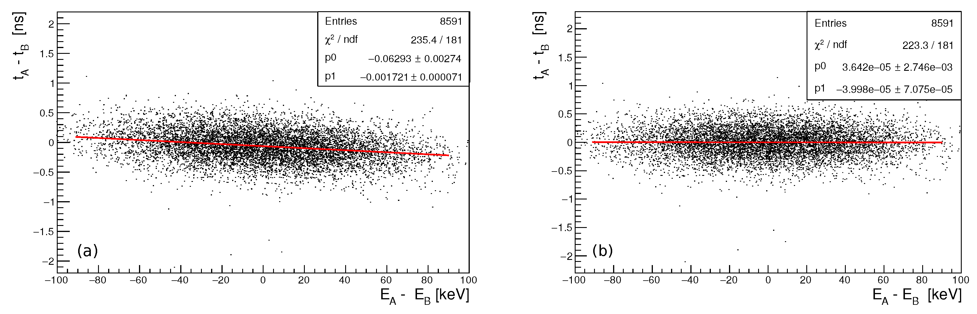
2.6.2. Walk Correction

It is known that the leading-edge timing method suffers from the so-called walk effect dependence of the threshold crossing time on the signal amplitude. For the coincidence time, $\Delta t=t_A-t_B$, this is translated into dependence on $E_A-E_B$, where $E_A$ and $E_B$ are total energies in modules A and B, respectively (Figure 8a). To correct the effect, we fit a first order polynomial $\Delta t=k\Delta E+l$ to data from which the slope k is determined. The corrected spectrum is obtained as:

$$\Delta t_c=\Delta t+k\Delta E$$

(17)

The $\Delta E-\Delta t$ diagram after applying this correction is shown in Figure 8b. This improves the coincidence time resolution by ∼ 4%.

2.6.3. Timing in Two-Pixel Events

In two-pixel Compton events, one can define the arrival time by two channels in each module. We have compared two approaches: in the first, we determine the time in each detector module as the simple average of the two pixel times:

$$t_m=\frac{t_{m,1}+t_{m,2}}{2}$$

(18)

where $m=\mathrm{A},\mathrm{B}$ and indices 1 and 2 refer to the two pixels fired in the module.

In the other approach, we determine the time in each module as a weighted average of the two pixel times:

$$t_m=t_{m,1}\frac{E_1}{E_m}+t_{m,2}\frac{E_2}{E_m}$$

(19)

where $m=\mathrm{A},\mathrm{B}$ and indices 1 and 2 refer to the two pixels fired in the module. As demonstrated in Figure 9, the latter method yields a better result.

3. Results

We investigated several aspects of detector performance in Compton scattering of 511 keV gamma particles: the ability to detect the Compton scattering events, including the reconstruction of the scattering angles $(\theta ,\varphi )$, as well as the corresponding energy and angular resolutions. We also tested the timing performance of two modules in coincident detection of two 511 keV gamma particles from positron annihilation.

3.1. Reconstruction of Compton Events

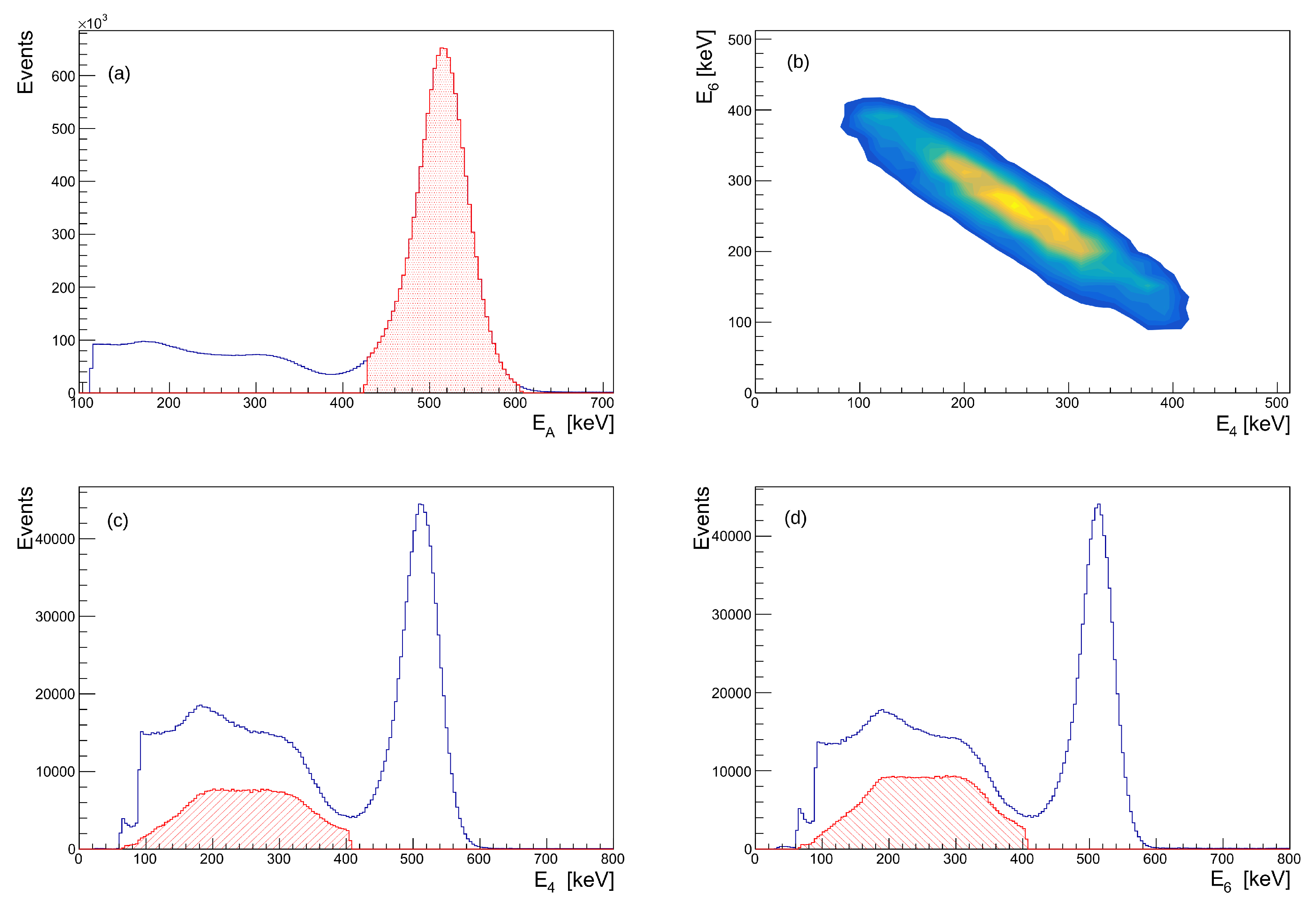
To select the events where Compton scattering occurs inside a module, we require that the total deposited gamma energy, defined as the sum of the fired pixels’ energies, is within the ±$3\sigma$ range from the peak maximum, as in Figure 10a. Generally, in those events, one or more pixels could have fired, contributing to the total energy. The relative abundances of events with different multiplicities of fired pixels are summarized in

Table 3. Abundance of events with different multiplicities relative to the total triggered events.

Events	Fraction of Events
Total triggered	1
Full energy deposition in the module	0.62
of which events with:
1 pixel fired	0.46
2 pixels fired	0.15
>2 pixels fired	0.01

. By selecting the events with two fired pixels and full energy deposition, we select the Compton scattered gammas. The obtained energies of contributing pixels are shown in Figure 10b–d.

3.2. Energy Resolution

The Compton events may have different event topologies in a detector module reflected in different mean inter-pixel distances, d, ranging from 3.2 mm for the adjacent pixels to 13.6 mm for the farthest pixel pairs (see Figure 1). A specific event topology can be chosen by selecting the corresponding pixel distance. The total gamma energy, reconstructed as the sum of the fired pixels’ energies, is shown in Figure 4a. One observes the shift of the position of the full energy peak depending on event topology. Most notably, the peak maximum is shifted upwards ∼30 keV for the events where the fired pixels are adjacent neighbors, while much lower shifts (<10 keV) are observed when the fired pixels are more distant neighbors. The observed shifts had been attributed to light sharing between the pixels [11]. A procedure to correct this effect and reconstruct the real energy depositions is presented in Section 2.4.2. Upon applying it, the gamma energies are correctly reconstructed for all event topologies, as demonstrated in Figure 4b.

The energy resolution at 511 keV, defined as the full width at half maximum of the energy sum peak, was 12.4% ± 0.1% for the Compton events, where the fired pixels are adjacent neighbors, and it was 12.0% ± 0.2% for the case where the fired pixels are farther neighbors. This is consistent with the observed mean energy resolution of single pixels, which was 12.2% ± 0.7%.

3.3. Angular Resolution

The scattering angle $\theta$ was reconstructed from the measured pixel energies using Compton scattering kinematics (see Section 2.5 for details). The reconstructed angles were in the range of ${40}^{\circ }<\theta <{90}^{\circ }$, as shown in Figure 11a, where the lower limit ($\theta ={40}^{\circ }$) was set by the pixel energy threshold, while the upper limit was determined by the reconstruction algorithm, which relies on suppression of the observed scattering at angles $\theta >{90}^{\circ }$, due to a lower cross-section and short attenuation length. The angular resolution was limited by the energy resolution of the pixels, and it was approximately constant throughout the acceptance, being $\Delta \theta \simeq {18.8}^{\circ }$ (FWHM).

The angle $\varphi$ was reconstructed from the relative positions of the two fired pixels. In this case, the module had a full $2\pi$ acceptance; however, it was non-uniform, because the scattered gammas were more attenuated at the angles covered by more distant pixel pairs, as shown in Figure 6. This can be corrected, as described in Section 2.5.3. Figure 11b shows an example of the acceptance-corrected $\varphi$ distribution for coincident Compton events in two modules. The angular resolution in $\varphi$ depends on the distance of the fired pixels, ranging from $\Delta \varphi ={12.7}^{\circ }$ (FWHM) for the largest pixel distance d to $\Delta \varphi ={54}^{\circ }$ (FWHM) when the fired pixels are adjacent neighbors.

3.4. Coincidence Time Resolution

The coincidence time resolution (CTR) of the system of two modules has been evaluated for events where Compton scattering occurs in both modules. In order to minimize the influence of events with incomplete energy absorption in a module, we required the energy in each module to be ±2$\sigma$ from the full energy peak. The arrival time of each signal was reconstructed by the leading edge method, on top of which we applied walk correction and pixel-to-pixel offset correction, described in detail in Section 2.6.1.

In Compton events, two fired pixels in each module can determine time, and we have examined two approaches to combine this information. In the first, the time in a module was determined as the arithmetic mean of the times reconstructed from pixels, while the second approach used the weighted mean, with weights corresponding to energy deposited in each pixel. The time difference between the modules $\Delta t=t_A-t_B$ is plotted in Figure 9. The first method resulted in $\Delta t=0.61\pm 0.02$ ns (FWHM), while the second method yielded $\Delta t=0.56\pm 0.02$ ns (FWHM). The latter is consistent with the result $\Delta t=0.54\pm 0.02$ ns (FWHM) obtained for single-pixel (photo-electric absorption) events, under the same operating conditions.

4. Discussion and Conclusions

We have presented the performance of the single-layer scintillator pixel detectors, demonstrating that it is possible to detect Compton scattered gamma particles with energy and timing resolutions comparable to those achieved in photo-electric absorption, while it is also possible to reconstruct the direction of the scattered gammas. The detection and full reconstruction of Compton scattering has been of interest in medical imaging, such as PET, where measurement of polarization correlations of annihilation quanta had been studied to improve sensitivity. This work proves the concept of the full Compton scattering reconstruction in modules with only one readout layer. Compared to two-layer Compton detectors, the number of electronic channels is reduced by a half; hence, the application of single-layer modules could have the potential to significantly improve the cost efficiency for larger devices with Compton detection capabilities.

References

- Kuncic, Z.; McNamara, A.; Wu, K.; Boardman, D. Polarization enhanced X-ray imaging for biomedicine. Nucl. Instrum. Methods Phys. Res. A 2011, 648, S208–S210. [Google Scholar] [CrossRef]
- McNamara, A.; Toghyani, M.; Gillam, J.; Wu, K.; Kuncic, Z. Towards optimal imaging with PET: An in silico feasibility study. Phys. Med. Biol. 2014, 59, 7587–7600. [Google Scholar] [CrossRef] [PubMed]
- Toghyani, M.; Gillam, J.; McNamara, A.; Kuncic, Z. Polarisation-based coincidence event discrimination: An in silico study towards a feasible scheme for Compton-PET. Phys. Med. Biol. 2016, 61, 5803–5817. [Google Scholar] [CrossRef] [PubMed]
- Mitani, T.; Tanaka, T.; Nakazawa, K.; Takahashi, T.; Takashima, T.; Tajima, H.; Nakamura, H.; Nomachi, M.; Nakamoto, T.; Fukazawa, Y. A prototype Si/CdTe Compton camera and the polarization measurement. IEEE Trans. Nucl. Sci. 2004, 51, 2432–2437. [Google Scholar] [CrossRef]
- Takeda, S.; Odaka, H.; Katsuta, J.; Ishikawa, S.; Sugimoto, S.; Koseki, Y.; Watanabe, S.; Sato, G.; Kokubun, M.; Takahashi, T.; et al. Polarimetric performance of Si/CdTe semiconductor Compton camera. Nucl. Instrum. Methods Phys. Res. A 2010, 622, 619–627. [Google Scholar] [CrossRef]
- Yonetoku, D.; Murakami, T.; Gunji, S.; Mihara, T.; Sakashita, T.; Morihara, Y.; Kikuchi, Y.; Takahashi, T.; Fujimoto, H.; Toukairin, N.; et al. Gamma-Ray Burst Polarimeter-GAP-aboard the Small Solar Power Sail Demonstrator IKAROS. Publ. Astron. Soc. Jap. 2011, 63, 625–638. [Google Scholar] [CrossRef]
- Shimazoe, K.; Yoshino, M.; Ohshima, Y.; Uenomachi, M.; Oogane, K.; Orita, T.; Takahashi, H.; Kamada, K.; Yoshikawa, A.; Takahashi, M. Development of simultaneous PET and Compton imaging using GAGG-SiPM based pixel detectors. Nucl. Instrum. Methods Phys. Res. A 2018. [Google Scholar] [CrossRef]
- Uenomachi, M.; Mizumachi, Y.; Yoshihara, Y.; Takahashi, T.; Shimazoe, K.; Yabu, G.; Yoneda, H.; Watanabe, S.; Takeda, S.; Orita, T.; et al. Double photon emission coincidence imaging with GAGG-SiPM Compton camera. Nucl. Instrum. Methods Phys. Res. A 2018. [Google Scholar] [CrossRef]
- Spillmann, U.; Bräuning, H.; Hess, S.; Beyer, H.; Stöhker, T.; Dousse, J.C.; Protic, D.; Krings, T. Performance of a Ge-microstrip imaging detector and polarimeter. Rev. Sci. Instrum. 2008, 79, 083101. [Google Scholar] [CrossRef] [PubMed]
- Bloser, P.F.; Legere, J.S.; McConnell, M.L.; Macri, J.R.; Bancroft, C.M.; Connor, T.P.; Ryan, J.M. Calibration of the Gamma-RAy Polarimeter Experiment (GRAPE) at a Polarized Hard X-Ray Beam. Nucl. Instrum. Methods Phys. Res. A 2009, 600, 424–433. [Google Scholar] [CrossRef]
- Makek, M.; Bosnar, D.; Gačić, V.; Pavelić, L.; Šenjug, P.; Žugec, P. Performance of scintillation pixel detectors with MPPC read-out and digital signal processing. Acta Phys. Pol. B 2017, 48, 1721–1726. [Google Scholar] [CrossRef]
- Gundacker, S.; Auffray, E.; Pauwels, K.; Lecoq, P. Measurement of intrinsic rise times for various L(Y)SO and LuAG scintillators with a general study of prompt photons to achieve 10 ps in TOF-PET. Phys. Med. Biol. 2016, 61, 2802–2837. [Google Scholar] [CrossRef] [PubMed]
- Berger, M.; Hubbell, J.; Seltzer, S.; Chang, J.; Coursey, J.; Sukumar, R.; Zucker, D.; Olsen, K. XCOM: Photon Cross Section Database (Version 1.5). Available online: http://physics.nist.gov/xcom (accessed on 30 January 2019).
Figure 1.
Schematic drawing of the scintillator pixel array: (a) front view; (b) side view.
Figure 2.
Examples of digitized detector signals; the distance between two samples on the X-axis corresponds to 625 ps: (a) the signal region where the baseline, the amplitude, and the integral are determined; (b) coincident signals from two detectors represented by circles (red) and squares (blue), respectively. The signal region at the beginning of the rising edge is shown. The time of the signal arrival is obtained from interpolation of the samples below and above the threshold, as marked by the red and the blue lines for the two signals, respectively.
Figure 3.
Observed correlation of energies between adjacent Pixel Nos. 5 and 6, attributed to light sharing.
Figure 4.
Observed energy of the fully absorbed 511 keV gamma: (a) two-pixel events before the light sharing correction; (b) two-pixel events after the light sharing correction.
Figure 5.
Reconstructed scattering angle versus response in: (a) lower-energy pixel; (b) higher-energy pixel.
Figure 6.
The normalized -acceptance for Compton scattering of 511 keV gammas in a module.
Figure 7.
Channel-to-channel timing variations: (a) before correction; (b) after correction.
Figure 8.
Coincidence time vs. energy difference , for Compton events. Histogram (a) shows the walk effect as a clear dependence between and . Histogram (b) is obtained after applying the walk correction.
Figure 9.
Coincidence time spectra for selected Compton events, after applying channel-by-channel and walk corrections. In (a) is shown the coincidence time spectrum calculated using the arithmetic mean. In (b) is the coincidence time spectrum calculated using the weighted mean.
Figure 10.
Compton event reconstruction: (a) Energy deposition in detector module A. The selected energy range corresponding to full energy deposition is shaded. (b) Energy in two pixels that fire in a Compton event; in this example, pixel 6 vs. pixel 4 (second neighbors). (c) Energy deposition in pixel 4, for all triggered events (full spectrum) and for filtered Compton events (shaded). (d) Energy deposition in pixel 6, for all triggered events (full spectrum) and for filtered Compton events (shaded).
Figure 11.
Example of reconstructed angles in Compton scattering: (a) the scattering angle ; (b) the angle (acceptance corrected).