
Horocycles of Light in a Ferrocell


1
Soft Matter Lab, School of Arts, Sciences and Humanities, University of São Paulo, São Paulo 03828-000, Brazil
2
Space Science Center, 235 Martindale Drive, Morehead State University, Morehead, KY 40531, USA
*
Author to whom correspondence should be addressed.
Condens. Matter 2021, 6(3), 30; https://doi.org/10.3390/condmat6030030
Submission received: 29 June 2021
/
Revised: 6 August 2021
/
Accepted: 7 August 2021
/
Published: 10 August 2021
Abstract
:We studied the effects of image formation in a device known as Ferrocell, which consists of a thin film of a ferrofluid solution between two glass plates subjected to an external magnetic field in the presence of a light source. Following suggestions found in the literature, we compared the Ferrocell light scattering for some magnetic field configurations with the conical scattering of light by thin structures found in foams known as Plateau borders, and we discuss this type of scattering with the concept of diffracted rays from the Geometrical Theory of Diffraction. For certain magnetic field configurations, a Ferrocell with a point light source creates images of circles, parabolas, and hyperboles. We interpret the Ferrocell images as analogous to a Möbius transformation by inversion of the magnetic field. The formation of circles through this transformation is known as horocycles, which can be observed directly in the Ferrocell plane.
1. Introduction
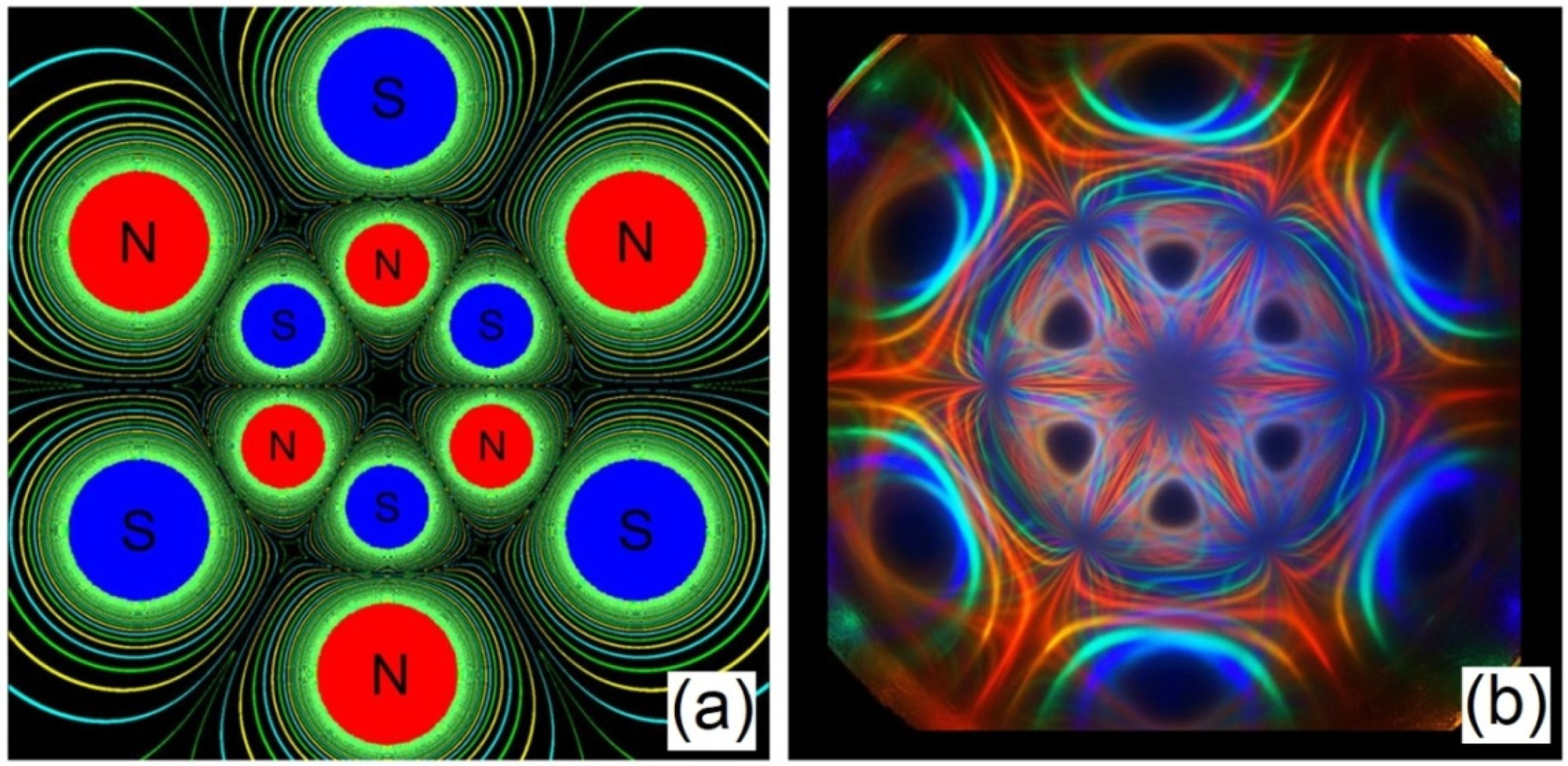
We can observe a curious case of directional light scattering in a Hele-Shaw cell filled with a ferrofluid solution known as Ferrocell as shown in Figure 1. The Ferrocell is subjected to a static external magnetic field, and for the specific case of ferrofluids, the magnetic field can alter structures formed by the agglomeration of nanoparticles that can scatter light [1,2,3,4,5,6]. In this way, we can have different conditions leading to diffraction, refraction, and reflection, for different configurations of magnetic fields, using field intensity and direction as control parameters, as well as cell thickness.
Systems similar to this one have been studied in the area of photonics in disordered media [7,8] for solar panels, in which diffraction patterns of polymeric wires forming different geometries present information on the distribution of wires. In these systems, effects such as Anderson localization are studied [9], where multiple scattering creates modes with a high level of spatial confinement, and has been reported in optical systems with ferrofluids. Other effects that can be explored for the case of light transport in the structures formed by ferrofluids when subjected to an applied magnetic field are light in photonic crystals [10,11], light polarization [12,13], and magnetic fluidic optical gratings [14,15], in which localized modes couple to transmission channels.
The understanding of light scattering in systems with ferrofluids, such as the case of Ferrocell, can lead to applications in the paint industry or new types of light sources such as Random lasers, leading to the development of new possibilities for fundamental research and the engineering of new devices [8]. Which leads to the question: what is the main mechanism in the light scattering in ferrofluids? For the case of ferrofluids subjected to an external magnetic field interacting with light, in general, we have a classic light scattering caused mainly by electric dipoles in the form of micro-needles that are aligned to an external magnetic field. Light scattering may be beyond disordered Gaussian scattering due to the fact that we have structures ordered by the magnetic field, such as diffraction gratings or photonic crystals leading to scattering resonances. However, some curious phenomena can be easily observed with the Ferrocell. In this article, we will discuss one of the concepts that most confuses some people in optics: the concept of diffracted rays [16,17,18,19], which is present at Ferrocell that is related to directional scattering. The name itself brings an oxymoron: rays in optics are often found in reflections and refractions, while diffraction is a characteristic seen in waves when they are deflected by obstacles. When faced with this phenomenon, some people may have a cognitive conflict, because the concepts of wave and ray are commonly used in separate scenarios, being considered only as an approximation to each other, but they cannot coexist, in the same way, as biologists who studied the platypus for the first time, were baffled by the observation of features of birds and mammals in the same animal. Historically, the problem of diffracted rays arises when Young analyzes Huygens‘ principle and ends up with Joseph Keller’s Geometrical Theory of Diffraction, in which along with the concept of a ray of geometrical optics, we have the concept of diffracted ray governed by rules analogous to those of reflection and refraction, in order to determine the resultant fields. This theory was later extended as the Uniform Theory of Diffraction [20,21], as a method for solving scattering problems for small discontinuities. This is a classic differential light scattering problem, in which different components of electrical and magnetic moments of light interacting with a material create anisotropic effects in the direction of the scattered light. The analysis of these effects is made by comparing some characteristic factors of the system with the wavelength of light, such as material properties and the scale of the scatterers. In some cases of scattering using Keller’s theory, light is considered to slip around obstacles.
In this paper, we will compare the patterns obtained with the scattering of light by a plane wave of a laser passing through the Ferrocell, with patterns observed directly in the Ferrocell plane and associate them with the concept of diffracted rays. To do this, we will first discuss the rays diffracted in a well-defined optical structure, known as the Plateau border, and then we will report the laser scattering on Ferrocell for different magnetic field orientations. After that, we will make a parallel between these patterns obtained with the laser and patterns observed directly in the Ferrocell plane for a light source with a spherical wavefront.
2. Diffracted Rays in Plateau Borders
A physical system that allows direct observation of diffracted rays is the scattering of a plane wave from a laser beam by a structure found in foams called the Plateau border and surface Plateau border [16,17,18,19]. The surface Plateau border is the place where a soap film meets a solid surface, for example, of a Plexiglass plate [17]. In this system, we have the simultaneous observation of reflection, refraction, and diffraction of light in a conical scattering. For a laser beam traveling in a plane perpendicular to the surface Plateau border in contact with a transparent plate of Figure 2, inclined radial 4°, we can see diffraction curves occurring in the same plane of incidence as the laser, with an interference figure between the laser beam and its reflection on the surface Plateau border. If we make the laser hit the Plateau border obliquely, the diffraction lines become curved.
The light scattering is done in these Plateau borders, which are confined in a transparent box. This box consists of two plain parallel Plexiglas plates separated by a gap (19.0 × 19.0 × 2.0 cm3). The box contains air and an amount of commercial dishwashing liquid diluted in water (V = 114 cm3). We have used Linear Alkylbenzene Sulfonate (LAS) as the surfactant, with a surface tension of 25 dyne/cm, and a density of ρ = 0.95 g/cm3. The refractive indices of detergent solution nl = 1.333, and ng = 1.0 for the air. We create the Plateau border by shaking the box. The length of the Plateau border is 2.0 cm, the profile of its cross-section is 0.5 mm across, and the detergent film thickness is 10 μm.
We verified that these curves are part of a conic diffraction that occurs exactly at half the apical angle of the cone, exactly as if it were the reflection angle of the incident ray, showing that we have a reflection/refraction occurring in diffraction angle, for different light wavelengths.
Unlike the case of diffraction in wires, we can directly follow the reflection in this system, through the most intense points called laser dogs (LD). These points are projections of the reflected beam. Note that all reflection points marked by laser dogs exactly coincide with the circular diffraction/interference line. The general equation for any conic section obtained by this scattering.
where A, B, C, D, E, and F are constants. Using the discriminant ∆ = B2 − 4AC, the profile of Equation (1) is an ellipse when A is different from C or B is equal to zero, or a circle if ∆ < 0 when A is equal C, a parabola when ∆ = 0 and hyperbola when ∆ > 0. This equation represents the possible luminous patterns obtained with the cone sections with a ϕ angle.
In Figure 3a we have the diagram of the laser beam incident on a Plateau border formed where three soap films meet in a Hele-Shaw cell with the formation of the parlaseric circle [16,17,18,19] on a screen perpendicular to the axis of the cone, which makes the parameter B in Equation (1) cancel out. The inset in Figure 3a shows that we are now looking at the projections of the cone in the plane with the red circle perpendicular to the axis of the cone, while the plane parallel to the axis of the cone with the green line showing a hyperbola applies to the case discussed in Figure 2.
In addition to the circular diffraction pattern, the images shown in Figure 3b present in some light patterns straight lines of diffraction associated with the Fraunhofer diffraction, which is characteristic of triangular obstacles due to the triangular shape of a Plateau border. Another important thing shown with these patterns is that while in Figure 2 we have only one reflected ray (LD) of the laser beam (LS) characteristic of geometric optics being crossed by a diffraction line, for the case of the patterns in Figure 3b we can have two reflected rays or four rays reflected on the diffraction circle. This is due to the fact that each soap film is like a beam splitter while diffracting light. For the case of circular patterns, one can prove that the angle of the reflected light rays is the same angle of the diffracted rays given by the angle of the cone ϕ.
With this experiment, we can observe some important characteristics in similar optical systems, as the projected patterns of the diffracted rays always cross the image of the light source, and also that the angles of the diffracted rays in the diffraction cone are identical to the reflection angles. In a previous work [6] we showed how a system with a grid of transparent wires can make analogous patterns with reflection and refraction of light, which creates patterns similar to the cat’s eye effect on gemstones.
3. Light Scattering in Ferrofluids
Now, we will apply these ideas of Geometrical Theory of Diffraction in the Ferrocell. Light scattering in ferrofluids has been debated over the last two decades, which shows the complexity of an interesting topic [22,23]. For example, light scattering by self-assembled arrays of ferrofluid micro-needles was compared to light scattering in cylinders [24]. Some authors suggest that the absence of spacing between fringes of diffraction patterns for the case of ferrofluids indicates that the observed pattern is caused by multiple diffractions by a spatial grating of magnetic chains with a combination of diffraction and interference [25].
The light source used in our next experiment is a green diode laser (10 mW) with a wavelength of 532 nm. The laser beam width is around 1.0 mm. The ferrofluid used in the experiment of the diagram of Figure 4a is the EFH1 (Ferrotec) with saturation magnetization of 440 G, and the ferrofluid solution prepared to be placed in Ferrocell is a solution with half EFH1 and half mineral oil, with 10 nm size single domain iron oxide nanoparticles. The ferrofluid solution is placed between two glass plates, with each glass plate having a thickness variation of around 1 μm, forming a thin film with a thickness of around 10 μm. The response time is of the order of 200 ms, and the scattering pattern disappears almost instantly after removing the magnetic field. The ferrofluid is isotropic for very low magnetic fields, and light passes through the Ferrocell shown in Figure 4b. When the magnetic field is increased, we can observe different patterns of light scattering in Figure 4c–f depending on the intensity and orientation of the magnetic field. The magnetic field in the region where the laser spot hits Ferrocell is created by permanent magnets and has its intensity and orientation measured with a gaussmeter as is shown in Figure 5. For the experiment in which we use a laser beam as a light source, the magnetic field can be considered uniform in the region where the laser hits the Ferrocell. For experiments where we use an incoherent light source, the magnetic field perpendicular to the Ferrocell plane is plotted on the X-Y plane intensity graphs at the bottom of Figure 5.
The light scattering is caused by structures formed in the ferrofluid in the presence of the magnetic field, ranging from 200 G to 1000 G, creating some elongated structures, known as needle-like structures shown in Figure 4g–i. The light scattering of this array of linear magnetic nanoparticle chains oriented by an external magnetic field shows components that involve both diffraction and reflection simultaneously according to the Geometrical Theory of Diffraction, such as the formation of luminous rings due to the existence of an angle between the incident light and the orientation of the magnetic field.
Increasing the angle between the incident laser beam and the magnetic field from 0° to 90° changes the light patterns in ferrofluids from a circle to a straight line as reported by some authors studying ferrofluids [24]. A very similar effect can be obtained using Ferrocell as shown in Figure 4, where we have the system without the magnetic field in Figure 4b, and with the presence of the magnetic field and changing the field orientation until the circle is formed in the sequence from Figure 4b–f. In the literature, we have found that light propagation in a system with small particles can be described by scattering matrix S(θ,ϕ) [26] with additional notation described in Ref. [27], and for the general case of an arbitrary scatterer illuminated by a plane electromagnetic wave propagating along the direction perpendicular to the Ferrocell plate, the amplitudes of electric field E of the scattered wave are represented by:
Based on the Geometrical Theory of Diffraction, the electric field EGTD has two components, one for the rays of geometric optics EGO and another for the diffracted rays ED:
According to Keller, when the incident rays in the direction of propagation of the incident wave are oblique to the edge of the obstacle, the diffracted wave is conical. The diffracted ray and the corresponding incident ray make equal angles with the obstacle. Considering the formation of image is related to the intensities of these vectors, based on Kirchhoff’s theory of diffraction, the electric field is associated with the diffracted field ue and the cone of diffracted rays is giving by [2]:
where K is the diffraction coefficient, ui is the incident field, r is the distance between the Ferrocell and the screen and k = 2π/λ is the wavenumber of the incident field with the wavelength λ. This field creates a pattern of diffracted rays of a right circular cone [24] as
where m is the inclination of the magnetic field in the point at which the laser touches the Ferrocell. This cone projected in a screen can form patterns described in Equation (1). Compared to scattering in a cylinder, the curvature of the scattering pattern is related to a scattering cone that was explained by Keller as if the waves were sliding down the micro-needle walls [20,21], using the concept of diffracted rays. The formation of the scattering pattern occurs due to the intersection between the screen and the scattering cone, which depends on the angle between the magnetic field and the direction of the incident light.
As the size of scatterers is important in the Geometrical Theory of Diffraction, we will now explore the involved scales of micro-needles in Ferrocell. Depending on the incidence of light, we can imagine the Ferrocell as a flat waveguide, containing a structure dependent on the orientation and intensity of the magnetic field. This structure is shown by forming columns of the size of tens to hundreds of micrometers as shown in Figure 4g–i.
By carefully adjusting the magnetic field so that it aligns with the incident light from the laser beam, we can study some physical properties of the micro-needles structures along with the direction of the magnetic field. The image of Figure 6a shows a diffraction pattern with the shape of a circle around the laser dot, representing a typical Airy diffraction pattern for a magnetic field perpendicular to the plane of the paper. By making an angle of 5° between the magnetic field and the laser beam, the scattering pattern becomes asymmetric, with some of the light scattered across the top of Figure 6b. Changing the angle between the laser and the magnetic field to 10°, in Figure 6c we have the Airy pattern giving way to an image with the laser’s midpoint flanked by two local minima, two local maxima followed by a halo. Increasing the angle between the magnetic field and the laser beam to 15° in Figure 6d, the halo increases in diameter. In Figure 6e the angle of the magnetic field is 25°, while in Figure 6f the angle of the magnetic field is 35°, with the sides of the diffraction figure having a parabolic profile. In Figure 6g, with an angle of 50°, we have a hyperbola-shaped diffraction figure, with the center point of the laser beam flanked by two local minima and two local maxima, which occupy the same position as the disk of Airy.
The columns or micro-needles have a characteristic size that can be measured using light diffraction, when we place a uniform magnetic field with the same direction as the light, by forming these Airy diffraction patterns, as shown in Figure 7. We observed that the diameters of ferrofluid micro-needles reaching up to 4.3 µm. According to some authors in the field of ferrofluids [23], light scattering is essentially of an electric dipole nature, while scatterers (micro-needles) are organized by a magnetostatic phenomenon.
How can this information help us? The most important fact here is that we know that a laser light point with a well-defined orientation can be mapped into a curve associated with a conical one as a function of the magnetic field properties due to the light’s scattering properties. Directly applying the Geometrical Theory of Diffraction, each light pattern corresponds to a conical diffraction with Ferrocell intersecting the light cone, which is directly connected with the light ring formation in the Ferrocell.
4. Formation of Horocycles of Light in Ferrocell
In addition to the laser light scattering imaging case discussed earlier, we have the backlight imaging case shown in the diagram of Figure 8a. For this case, we can use a light source such as a LED or a light source projected on a light diffuser to create an approximately spherical light source. Direct observation of Ferrocell by a viewer also shows this transformation of a luminous point into a curve as a function of the magnetic field of Figure 8b.
The difference for this case, in comparison with the previous case using a laser beam, is that for this type of illumination we use a light source that creates a spherical wavefront and the control parameter associated with pattern formation must consider the position of the observer. As discussed previously, the formation of the luminous pattern can be interpreted as a contribution of multiple reflection, refraction, diffraction, and interference of light, forming a complex distribution of light intensities. The intensity of the luminous ring obtained with Ferrocell can be seen in Figure 8c. As in the case of Gaussian surfaces that are chosen to explore the symmetries of a charge distribution to simplify the calculation of a field in electrostatic problems, by choosing certain configurations of light sources, we can explore the magnetic field symmetries to predict the pattern observed in Ferrocell. In this way, exploring some symmetry properties of light sources positioning along with the magnetic field structure, we can compose one phenomenological model based on light-scattering properties that form sections of conic curves. For the regions close to the poles of the magnets, as it is shown in Figure 9a, we have the formation of internal tangent circles for a luminous configuration of the light sources in line. Using the same lighting arrangement, but now with a dipole magnetic field configuration of Figure 9c, we see the formation of internal tangent ellipses, with a parabolic boundary, a faded region followed by a hyperbolic boundary, where the lit region starts over.
Considering the position of the observer, we can see that the formation of luminous circles usually includes the region close to one of the poles of the magnet and the light source. In the case of the configuration of the dipole magnetic field, we notice the formation of ellipses, circles, parabolas, and hyperboles. This led us to investigate pattern formation with a single spherical light source in the presence of a dipole magnetic field configuration, changing the position of the observer. By varying the observer’s position, we see in Figure 10a a succession of patterns that start with a point when the observer is aligned with the light source and directly perpendicular to the magnetic field. As the observer increases its inclination with respect to the magnetic field, we see the formation of circles that evolve into ellipses that distort until the formation of open curves similar to parabolas.
These patterns can be reinterpreted as the intersection of luminous conics with the plane defined by the Ferrocell as the diagrams shown in Figure 11 [28]. For this luminous configuration in the presence of the magnetic field of a magnet, we have considered this conical section forming an optical field with bipolar symmetry, which is a two-dimensional system of coordinates, which can be considered as the projections in a plane.
Using this idea, we will make an approximation, in which we can explore the topological properties of the transformation of the magnetic field into a magneto-optical projection. A fundamental property of the magnetic field is that field lines do not intersect, and the properties of a field are normally preserved when it is mapped to the new coordinate system, so let us focus on the light patterns obtained by Ferrocell which do not have crossovers. From our experimental observations, the most suitable setup to achieve this is a direct linear array of light sources, such as a strip of LEDs. The transformations from the magnetic field to light images at Ferrocell bring us to the case of a mapping known as Möbius transformations [29,30], given by:
where a, b, c and d are complex constants.
From the set of available Möbius transformations, the image formation of the internal tangent circles is directly linked to the case of complex inversion of the surface of a sphere projected in a plane, from the point of view of projective geometry, with the transformation:
The bipolar coordinate system is based in two foci, and in a Cartesian system if the foci are taken to lie in each pole of the magnet at (−a,0) and (a,0):
The image of z under complex inversion has new length that is the reciprocal of the original, and the new angle is the negative of the original presented in Figure 12. The coordinate v ranges from to , and u ranges from 0 to . We may set up a one-to-one correspondence between the magnetic field and the optical field like the diagram of Figure 12b. For example, the following identities show that curves of constant u and v are circles in x-y space:
We can go from a Cartesian system to a bipolar system considering the reciprocal relations giving the transformations of Figure 12c,d forming τ isosurfaces [31,32]:
and
To illustrate the F transformation, let’s show the transformation of three blue circles through an inversion of Figure 12, creating the light blue circles: in Figure 12c, a second blue circle is inverted, obtaining the smaller circle within the dotted circular line that defines the inversion region. Taking a second circle concentric with the first dark blue circle in Figure 12d, we obtain a light blue tangent circle. In Figure 12e, we have another inversion, getting a larger circle and τ isosurfaces.
With this information, we can consider that the patterns obtained with Ferrocell can be approximated for the physical case in which we have a transformation of light sources in a line of Figure 13a–c that undergoes a light scattering into micro-needles aligned with the magnetic field, and this scattering creates luminous images in the plane of the Ferrocell that are perpendicular to both the incident light wave and the magnetic field. In this way, the magnetic field is linked to the light patterns by this transformation, just as the reciprocal space mapping of the X-ray diffraction patterns provides information about the crystal structure of materials.
The curves represented by Equation (9) can be associated with horocycles [30,31,32,33,34]. A horocycle is a curve in hyperbolic geometry whose normal or perpendicular geodesics all converge asymptotically in the same direction. Simulation of a sequence of luminous horocycles for the polar configuration in Figure 13d, similar to the experiment obtained in Figure 9a. We have a comparison between the experimental case of the F transformation applied to the case of a dipolar field in Figure 14a and a simulation for this case in Figure 14b.
In Figure 15a,b, we show that the crossing of the light scattering lines occurs due to the location of the light sources for the case of monopolar configuration. This does not mean that the magnetic field lines that gave rise to the pattern are crossing, but that the crossing is only because of a choice of overlapping light sources. In Figure 15c, we present the magnetic pattern perspective for the dipole configuration depicted in Figure 14 for light sources forming cross lines.
This leads us to question how conical scattering using the laser can be equivalent to direct observation scattering by a spherical light source in Ferrocell. A possible answer can be given if we consider light scattering in systems with geometric optics. If we consider the case of the purely geometric optics of a light ray hitting a cylinder obliquely with incidence angles θi and αi, we have multiple internal γ reflections and a sequence of refractions with transmitted T and refracted rays R with output angles αt,r and θt,r as shown in the diagrams in Figure 16a, with the light rays coming out of the cylinder in an approximately conical shape, as we can see in Figure 16b. An experimental demonstration of this quasi-cone using a red laser and a glass cylinder can be seen in Figure 16c.
In this case, we just have the laws of reflection and refraction of geometric optics, and we can use the representation of ray optics. Considering a grid of parallel cylinders of Figure 17a, we can observe the effect of pattern formation for a light bulb in different perspectives of this system in Figure 17b,c. Each cylinder of these grids acts as a conical scatterer for the multiple light rays coming from each lamp. The observer perceives that the light streak crosses the image of the light source, in this case where reflection and refraction occur simultaneously.
In this system, we have light scatterers formed by cylinders in an arrangement of parallel grids. In the first demonstration, the light pattern is a light streak perpendicular to the orientation of the scatterers, as we saw for the case of light diffraction in Figure 4c which occurs in the direction perpendicular to the direction of the applied magnetic field.
In a previous work [6], we showed other types of cylindrical grids forming other patterns and discussed their relationship with gem optics for the Chatoyance effect. In Figure 17c, we have another arrangement of transparent cylinders with four lamps, with a perspective forming a very inclined viewing angle, showing another luminous pattern, with projections of conical sections in an inverted V shape. Figure 17b,c show a version of geometric optics analogous to the diffraction cases of Figure 2. We can notice in this demonstration of Figure 17c that the lines of the light patterns intersect at some points. This allows us to understand that light patterns also depend on the viewer’s perspective, in addition to the alignment of grid elements.
In the case of Ferrocell, these facts emphasize that light scattering patterns are magneto-optical patterns, affected by the magnetic field that orients an array of particles in the same way as a diffraction grating, in addition to the observer’s perspective of the light source.
Another pattern formation comparison between a point light source and a laser beam is shown in Figure 18. In Figure 18c, we are presenting a pattern obtained by the scattering laser beam by refraction in a glass plate with a rectangular lattice and in Figure 18d with a hexagonal lattice. In Figure 18e, we have the direct observation of the pattern obtained on the glass plate with the rectangular lattice of Figure 18a, placing a spherical light source before the glass plate, and in Figure 18f for the case of the hexagonal lattice pictured in Figure 18b. We can see that the structure of the image is similar for both observation modes, similar to the case of patterns obtained in Ferrocell by laser scattering projected onto a screen or direct observation, and consequentially, these two observation modes are equivalent.
These experiments show how we can explore some of the properties of ferrofluids using the magneto-optical device known as a Ferrocell for direct observation of patterns and their connection with different concepts in optics. Other possibilities can be explored in different contexts in the future. For example, the formation of luminous halos in ferrofluids can be found in systems based on the thermal lens effects, without the application of an external magnetic field [35], or that is possible to observe structural changes in the solution of ferrofluid applying an external electric field [36]. Other interesting applications involve the development of sensors [37] and new optical elements [38].
5. Conclusions
In this work, we presented a phenomenological model for the pattern formation observed in a thin film of ferrofluids based on the Geometrical Theory of Diffraction and hyperbolic geometry. To simplify our approach, we began our discussion by presenting light scattering experiments on foam structures known as Plateau borders and the formation of the parlaseric circle in order to present the concept of diffracted rays.
After that, we investigated the light scattering in the Ferrocell subjected to a magnetic field in the presence of light sources. For different orientations of the magnetic field with respect to light propagation, it is possible to observe different types of light scattering. In one case, we can obtain Airy patterns that are related to the diameter of the micro-needles, or a second type of scattering, in which we have diffracted rays from a conical scattering. We have observed that in this system, there are structures formed by nanoparticles with lengths on the order of hundreds of micrometers and diameters of few micrometers, which interacts with an electromagnetic wave with wavelengths in the visible range.
As in the case of Gaussian surfaces that are chosen to explore the symmetries of a charge distribution to simplify the calculation of a field in electromagnetism, by choosing certain configurations of light sources, we can explore the magnetic field symmetries to predict the pattern observed in Ferrocell, in which a light source is partially transformed to a luminous ring.
We also present some experiments in geometric optics with light-scattering in cylinders and stamped plates to show the connection between the conical scattering described in the Geometrical Theory of Diffraction theory and geometric optics.
We can interpret these patterns as conical sections formed by the conical scattering of light that crosses the Ferrocell plane if we orient the light source in one of the symmetry axes of the magnetic field. Using some concepts of hyperbolic geometry, we can consider light patterns as Möbius transformations of the magnetic field for certain configurations of light sources. One of these patterns, a ring-shaped light pattern, is associated with the horocycle, which is an element found in hyperbolic geometry.
Author Contributions
All authors contributed to prepare the experiments, propose the mechanisms involved, and analyze the results. Preparation of this manuscript, A.T. and A.P.B.T.; conceptualization, A.T. and A.P.B.T.; methodology, A.T. and A.P.B.T.; software, A.T., A.P.B.T. and M.S.; editing, A.T., A.P.B.T., M.S. All authors have read and agreed to the published version of the manuscript.
Funding
This work was partially supported by Conselho Nacional de Desenvolvimento Científico e Tecnológico (CNPq), Instituto Nacional de Ciência e Tecnologia de Fluidos Complexos (INCT-FCx), and by Fundação de Amparo à Pesquisa do Estado de São Paulo (FAPESP) FAPESP/CNPq#573560/2008-0.
Institutional Review Board Statement
Not applicable.
Informed Consent Statement
Not applicable.
Data Availability Statement
Not applicable.
Acknowledgments
A.T. and A.P.B.T. thank Conselho Nacional de Desenvolvimento Científico e Tecnológico (CNPq), Instituto Nacional de Ciência e Tecnologia de Fluidos Complexos (INCT-FCx), and Fundação de Amparo à Pesquisa do Estado de São Paulo (FAPESP). The authors also thank Doug Hatley for the development of diagrams and videos used in this research.
Conflicts of Interest
The authors declare no conflict of interest.
References
- Tufaile, A.; Tufaile, A.P.B. Ferrocell and Magnetic Patterns—Illustrations of Concepts, Experiments and Demonstrations. 2021. Available online: 10.6084/m9.figshare.14485392.v1 (accessed on 1 June 2021).
- Tufaile, A.; Vanderelli, T.A.; Tufaile, A.P.B. Observing the Jumping Laser Dogs. J. Appl. Math. Phys. 2016, 4, 1977–1988. [Google Scholar] [CrossRef] [Green Version]
- Tufaile, A.; Vanderelli, T.A.; Tufaile, A.P.B. Light polarization using ferrofluids and magnetic fields. J. Adv. Condens. Matter Phys. 2017, 2017, 2583717. [Google Scholar] [CrossRef] [Green Version]
- Tufaile, A.; Vanderelli, T.A.; Snyder, M.; Tufaile, A.P.B. Observing Dynamical Systems Using Magneto-Controlled Diffraction. Condens. Matter 2019, 4, 35. [Google Scholar] [CrossRef] [Green Version]
- Tufaile, A.; Tufaile, A.P.B.; Vanderelli, T.A.; Snyder, M. Investigation of Light Patterns in a Ferrolens Subjected to a Magnetic Field; OSA Publishing: Washington, DC, USA, 2019. [Google Scholar]
- Tufaile, A.; Snyder, M.; Vanderelli, T.A.; Tufaile, A.P.B. Jumping Sundogs, Cat’s Eye and Ferrofluids. Condens. Matter 2020, 5, 45. [Google Scholar] [CrossRef]
- Kelzenberg, M.D.; Boettcher, S.; Petykiewicz, J.A.; Turner-Evans, D.; Putnam, M.C.; Warren, E.; Spurgeon, J.M.; Briggs, R.M.; Lewis, N.S.; Atwater, H.A. Enhanced absorption and carrier collection in Si wire arrays for photovoltaic applications. Nat. Mater. 2010, 9, 239–244. [Google Scholar] [CrossRef]
- Wiersma, D. Disordered photonics. Nat. Photon. 2013, 7, 188–196. [Google Scholar] [CrossRef]
- Shalini, M.; Ramachandran, H.; Kumar, N. Localization of Light by Magnetically Tuned Correlated Disorder: Trapping of Light in Ferrofluids. Available online: https://www.chemistryworld.com/news/scientists-trap-light-in-nano-soup/3003544.article (accessed on 1 June 2021).
- Yang, S.; Horng, H.; Shiao, Y.; Hong, C.-Y.; Yang, H. Photonic-crystal resonant effect using self-assembly ordered structures in magnetic fluid films under external magnetic fields. J. Magn. Magn. Mater. 2006, 307, 43–47. [Google Scholar] [CrossRef]
- Pu, S.; Liu, M. Magnetically tunable two-dimensional photonic crystal by self-assembling in magnetite magnetic fluid. In Proceedings of the 2008 2nd IEEE International Nanoelectronics Conference, Shanghai, China, 24–27 March 2008; pp. 210–213. [Google Scholar]
- Zhao, Y.; Ying, Y.; Wang, Q.; Hu, H.-F. Simulation on Microstructure and Optical Property of Magnetic Fluid Photonic Crystal. IEEE Trans. Magn. 2014, 50, 1–12. [Google Scholar] [CrossRef]
- Vales-Pinzón, C.; Alvarado-Gil, J.J.; Medina-Esquivel, R.; Martínez-Torres, P. Polarized light transmission in ferrofluids loaded with carbon nanotubes in the presence of a uniform magnetic field. J. Magn. Magn. Mater. 2014, 369, 114–121. [Google Scholar] [CrossRef]
- Ying, Y.; Xu, K.; Si, G.-Y. Simulation and experiment study of a new type magnetic fluid optical grating. Optik 2019, 202, 163561. [Google Scholar] [CrossRef]
- Tarjányi, N.; Káčik, D. Dichromatic properties of a magnetic fluid thin layer. Optik 2021, 244, 167562. [Google Scholar] [CrossRef]
- Tufaile, A.P.B. Parhelic-like circle from light scattering in Plateau borders. Phys. Lett. A 2015, 379, 529–534. [Google Scholar] [CrossRef] [Green Version]
- Tufaile, A.P.B.; Tufaile, A. The dynamics of diffracted rays in foams. Phys. Lett. A 2015, 379, 3059–3068. [Google Scholar] [CrossRef]
- Fitzgerald, R.J. Soap halos. Phys. Today 2019, 72, 68. [Google Scholar] [CrossRef]
- Conover, E. Researchers Create Laser Dogs with Soap Bubbles, Science. Available online: http://news.sciencemag.org/physics/2015/02/researchers-create-laser-dogs-soap-bubbles (accessed on 1 June 2021).
- Croswell, W.; Bucci, O.M.; Pelosi, G. From wave theory to ray optics. IEEE Antennas Propag. Mag. 1994, 36, 35–42. [Google Scholar] [CrossRef]
- Rahmat-Samii, Y. GTO. UTO, UAT, and STO: A Historical Revisit and Personal Observations. IEEE Antennas Propag. Mag. 2013, 55, 29–40. [Google Scholar] [CrossRef]
- Philip, J.; Laskar, J.M. Optical Properties and Applications of Ferrofluids—A Review. J. Nanofluids 2012, 1, 3–20. [Google Scholar] [CrossRef]
- Dave, V.; Mehta, R.; Bhatnagar, S. Extinction of light by a Ferrocell and ferrofluid layers: A comparison. Optik 2020, 217, 164861. [Google Scholar] [CrossRef]
- Laskar, J.M.; Brojabasi, S.; Raj, B.; Philip, J. Comparison of light scattering from self assembled array of nanoparticle chains with cylinders. Opt. Commun. 2012, 285, 1242–1247. [Google Scholar] [CrossRef]
- Malynych, S.Z.; Tokarev, A.; Hudson, S.; Chumanov, G.; Ballato, J.; Kornev, K.G. Magneto-controlled illumination with opto-fluidics. J. Magn. Magn. Mater. 2010, 322, 1894–1897. [Google Scholar] [CrossRef]
- Mehta, R. Polarization dependent extinction coefficients of superparamagnetic colloids in transverse and longitudinal configurations of magnetic field. Opt. Mater. 2013, 35, 1436–1442. [Google Scholar] [CrossRef]
- Van De Hulst, H.C.; Twersky, V. Light Scattering by Small Particles. Phys. Today 1957, 10, 28–30. [Google Scholar] [CrossRef]
- Ramsden, P. Conic Sections: The Double Cone. Wolfram Demonstrations Project. 2011. Available online: https://demonstrations.wolfram.com/ConicSectionsTheDoubleCone/ (accessed on 1 June 2021).
- Tufaile, A.P.B.; Tufaile, A. Hyperbolic prisms and foams in Hele-Shaw cells. Phys. Lett. A 2011, 375, 3693–3698. [Google Scholar] [CrossRef]
- Shiu, P.; Needham, T. Visual Complex Analysis. Math. Gaz. 1999, 83, 182. [Google Scholar] [CrossRef] [Green Version]
- Weisstein, E.W. Bipolar Coordinates. from MathWorld—A Wolfram Web Resource. Available online: https://mathworld.wolfram.com/BipolarCoordinates.html (accessed on 1 June 2021).
- Bipolar Coordinates, Wikipedia. Available online: https://en.wikipedia.org/wiki/Bipolar_coordinates (accessed on 1 June 2021).
- Church, G. Mobius Transformations of Lines and Circles, Geogebra. Available online: https://www.geogebra.org/m/DR64X4VX (accessed on 1 June 2021).
- Horocycles of Light, Adriana Tufaile, YouTube. Available online: https://youtu.be/U7FzyYVvdNY (accessed on 29 July 2021).
- Wang, H.; Pu, S.; Gharibi, A.; Wang, N. Generation and versatile transmission properties of ring-shaped beams based on thermal lens effect of magnetic fluids and ring-limited windows. Opt. Commun. 2013, 286, 211–216. [Google Scholar] [CrossRef]
- Beketova, E.S.; Nechaeva, O.A.; Mkrtchyan, V.D.; Zakinyan, A.R.; Dikanskii, Y.I. Structural Transformations in Magnetic Emulsions upon Their Inter-action with an Alternating Electric Field. Colloid J. 2021, 83, 189–202. [Google Scholar] [CrossRef]
- Li, Y.; Pu, S.; Hao, Z.; Yan, S.; Zhang, Y.; Lahoubi, M. Vector magnetic field sensor based on U-bent single-mode fiber and magnetic fluid. Opt. Express 2021, 29, 5236–5246. [Google Scholar] [CrossRef] [PubMed]
- Zakinyan, A.A.; Belykh, S.S.; Yerin, K.V. Structured media based on magnetic colloids as a promising material for magnetically controllable optical elements. J. Opt. Technol. 2021, 88, 158–165. [Google Scholar] [CrossRef]
Figure 1.
Static arrangement of magnets and light pattern from a Ferrocell. Arrangement of twelve magnets with their respective isopotentials in (a) to demonstrate the applied magnetostatic field used in (b), where we have a luminous pattern obtained with a Ferrocell with the illumination of various colors in a circular arrangement.

Figure 2.
An example of how we can go from diffraction to conical diffraction with diffracted rays using a green laser and the structure present in soap bubbles known as the Plateau border, tilting the angle of incidence of light φ (23°, 0°, and 20°). Using the angle
θ
of 4° to show the difference between the transmitted beam (LS) and the reflected beam (LD), therefore there is 8° between LS and LD. We can see that the diffraction cone also presents the reflection and refraction of light, which shows that we have the presence of the concept of diffracted rays. Light patterns are projections of parabolas from the conical scattering of light.

Figure 3.
Conic light diffraction diagram showing the incidence angle ϕi and the half apical angle of the light scattering cone ϕ in (a). The relationship between the angle of incidence of light and the formation of the scattering cone is the identity line or line of equality, with the formation of the parlaseric circle on a screen placed perpendicular to the axis of the cone in (b).

Figure 4.
Diagram showing the formation of diffracted rays in Ferrocell in (a), using a laser and an external magnetic field. Images of the scattering pattern projected on a screen: in (b) without an external magnetic field, in (c) magnetic field perpendicular to the laser propagation line, in (d) a magnetic field inclined 60° to the laser, in (e) a field with 45° inclination, and 10° inclination of the magnetic field in (f). Images obtained with the microscope showing the patterns of the micro-needles for different values of the magnetic field: in (g) without magnetic field, in (h) 200 G, and (i) 600 G.

Figure 5.
The source of the magnetic field is made using neodymium super magnets, which are placed close to the Ferrocell. In (a) we have the diagram for measuring the magnetic field in the monopolar configuration using a Hall sensor, the field strength perpendicular to the Hall sensor in a line, and a graph of the magnet field strength distribution in space. In (b) we have the diagram for measuring the magnetic field perpendicular to the Hall sensor in the dipolar configuration, the magnetic field intensity graph for the dipolar configuration from the center of the magnet, and the distribution of the magnetic field in space in the dipolar configuration.

Figure 6.
We can observe the formation of Airy diffraction patterns for the case in which we have the magnetic field aligned with the propagation direction of the laser beam, as shown in (a), which is perpendicular to the page. This pattern is related to the diameter of the micro-needles formed with the application of the magnetic field. The arrow on each image shows the angle between the laser and the magnetic field that is perpendicular to the page. By increasing the angle between the magnetic field and the laser beam shown in the inset of each figure, the light pattern obtained is similar to the case discussed for the case of parlaseric rays obtained with Plateau borders, with 5°in (b), 10° in (c), and 15° in (d) with the Airy diffraction image along with the diffracted ray circle at the same time. In (e) the angle between the laser and magnetic field is 25°, and in (f) we have a parabolic profile, along with the laser point with two minimum points for an angle of 35°. In the last light pattern in (g), we can observe only two minimums of intensity beside the central light point of the laser, which occupied the place of the minimum region of the Airy disk shown in (a). Next, to each low point are two local maximum intensity points in (g) for the angle of 50°. Ferrofluid images for 0° in (h), 17° in (i), 40° in (j), and 60° in (k).

Figure 7.
(a) Image obtained with a microscope of the micro-needle distribution in Ferrocell for a magnetic field perpendicular to the plane of the plate together with the diagram for the Airy pattern obtained by diffracting a 532 nm green laser. With this apparatus, we can measure the diameter of micro-needles. (b) Theoretical and experimental Airy patterns obtained with Ferrocell with an external magnetic field of 400 G and with a field of 600 G. The average diameter d of the micro-needles is around 4.3 μm. In (c), we have the intensity graph and these plots were obtained transforming the images in grayscale.

Figure 8.
The horocycle: diagram of the experiment to observe the luminous ring pattern is shown in (a). The luminous pattern obtained in the plane of the Ferrocell plate in (b) and luminous intensity graph of the same pattern in (c). We see the maximum intensity for the light source, while the light intensity varies in the rest of the light ring.

Figure 9.
The light pattern in (a) obtained with Ferrocell for a straight linear array of light sources aligned with the magnetic field lines for a monopolar configuration, which means that one of the magnet poles is in direct contact with the Ferrocell, forming inner tangent circles. In (b) we have different curves as intersection projections of a plane with a cone indicating in each one its eccentricity e: the straight line (e = infinity), the hyperbola (e = 2), the parabola (e = 1), the ellipse (e = 0.5) and the circle (e = 0). In (c), a partial image of a light pattern on Ferrocell was obtained with the straight arrangement of light sources aligned with the magnetic field for the case of a bipolar configuration, showing curves associated with the hyperbola, the parabola, and the ellipse.

Figure 10.
Light patterns were obtained through direct observation of Ferrocell with the spherical light source remaining on one of the symmetry lines of the magnetic field. As was seen with laser light scattering, we can see the evolution of the light pattern depending on the φ angle starting with a point in (a) for ϕ = 2°, passed to a circle in (b) for ϕ = 18°, evolving into an ellipse in (c) for ϕ = 27°, in (d) for ϕ = 31°, in (e) for ϕ = 37°, in (f) for ϕ = 42°, changing to an open curve in (g) for ϕ = 53°, giving way to a parabola in (h) for ϕ = 69° and a more open parabola in (i) for ϕ = 77°, as the viewer’s angle of view φ tilts relative to the plate.

Figure 11.
Diagrams showing conic sections obtained through the intersection of a plane with cones, starting with an ellipse (a), passing through a parabola (b), a hyperbola in (c), and straight lines in (d). If we consider the cone scattering discussed above and the plane formed by Ferrocell, the light patterns are formed at the intersection between the scattering cone and the Ferrocell plane.

Figure 12.
In (a), we have the diagram showing the superposition of the monopolar magnetic field with the diagram of the light patterns obtained for the straight array of light sources. Searching in the literature, we observed that the transformation F that takes the magnetic field pattern can be done through a Möbius transformation in which a sphere inverts the isopotentials of a polar field, known as a sphere inversion, as shown in (b). This F transformation is similar to the one which occurs when mapping between a polar coordinate system to a bipolar coordinate system. To illustrate the F transformation, let us show the transformation of three blue circles through an inversion, creating the light blue circles: in (c), a second blue circle is inverted, obtaining the smaller circle within the dotted circular line that defines the inversion region. Taking a second circle concentric with the first dark blue circle in (d), we obtain a light blue tangent circle. In (e), we have another inversion, getting a larger circle.

Figure 13.
A sequence of images showing the formation of circles from light sources positioned in a line of symmetry of the magnetic field, removing the most internal sources so that we can observe the internal profile of the light pattern, using the blue color from (a–c). Simulation of the light pattern in (d)with light sources represented by rounded rectangles aligned with an axis of symmetry of the light field, forming the inner tangent circles in Figure 9a.

Figure 14.
The light pattern on Ferrocell for a dipolar field in (a) and the simulation of this field using a Möbius inversion approximation in (b).
Figure 14.
The light pattern on Ferrocell for a dipolar field in (a) and the simulation of this field using a Möbius inversion approximation in (b).

Figure 15.
Light sources crossed configuration in the presence of a monopolar magnetic field in (a,b), we have intersecting light patterns. The perspective of the magnetic pattern for the dipolar configuration of Figure 14 for light sources forming crisscross lines in (c). This shows that mapping the magnetic field into a magneto-optical light pattern depends on the perspective of the viewer.

Figure 16.
(a) A light ray hitting a cylinder obliquely with incidence angles θi and αi, we have multiple internal γ reflections and a sequence of refractions with transmitted T and refracted rays R with output angles αt,r and θt,r as shown in the diagrams in (a), with the light rays coming out of the cylinder in an approximately conical shape with a scattering, as we can see in (b). An experimental demonstration of this cone can be seen in (c).

Figure 17.
In (a), the diagram of a grid of cylinders between two light bulbs and an observer. In (b), a demonstration of this optical system, with a light streak forming a pattern that passes through the image of the light source. In (c), a similar system with four light bulbs with a grazing angle of view, forming conical sections light patterns, making a multiple crossing.

Figure 18.
(a) Picture of a stamped glass plate with a rectangular pattern. (b) Picture of a stamped glass plate with a hexagonal pattern. In (c,d), the projections onto a screen of a laser beam are scattered by these two plates. In (e,f), direct observation of a point light source passing through each glass plate. We can see that both the projection on the screen and the direct observations form similar patterns.

Publisher’s Note: MDPI stays neutral with regard to jurisdictional claims in published maps and institutional affiliations. |
© 2021 by the authors. Licensee MDPI, Basel, Switzerland. This article is an open access article distributed under the terms and conditions of the Creative Commons Attribution (CC BY) license (https://creativecommons.org/licenses/by/4.0/).
Share and Cite
MDPI and ACS Style
Tufaile, A.; Snyder, M.; Tufaile, A.P.B. Horocycles of Light in a Ferrocell. Condens. Matter 2021, 6, 30. https://doi.org/10.3390/condmat6030030
AMA Style
Tufaile A, Snyder M, Tufaile APB. Horocycles of Light in a Ferrocell. Condensed Matter. 2021; 6(3):30. https://doi.org/10.3390/condmat6030030
Chicago/Turabian StyleTufaile, Alberto, Michael Snyder, and Adriana Pedrosa Biscaia Tufaile. 2021. "Horocycles of Light in a Ferrocell" Condensed Matter 6, no. 3: 30. https://doi.org/10.3390/condmat6030030