Full Statistics of Conjugated Thermodynamic Ensembles in Chains of Bistable Units

Abstract

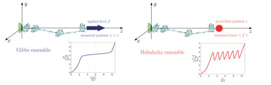
The statistical mechanics and the thermodynamics of small systems are characterized by the non-equivalence of the statistical ensembles. When concerning a polymer chain or an arbitrary chain of independent units, this concept leads to different force-extension responses for the isotensional (Gibbs) and the isometric (Helmholtz) thermodynamic ensembles for a limited number of units (far from the thermodynamic limit). While the average force-extension response has been largely investigated in both Gibbs and Helmholtz ensembles, the full statistical characterization of this thermo-mechanical behavior has not been approached by evaluating the corresponding probability densities. Therefore, we elaborate in this paper a technique for obtaining the probability density of the extension when force is applied (Gibbs ensemble) and the probability density of the force when the extension is prescribed (Helmholtz ensemble). This methodology, here developed at thermodynamic equilibrium, is applied to a specific chain composed of units characterized by a bistable potential energy, which is able to mimic the folding and unfolding of several macromolecules of biological origin.

1. Introduction

The recent developments of thermodynamics and statistical mechanics concern the thermodynamics of small systems, kept far from the thermodynamic limit, and the stochastic thermodynamics, which is based on Langevin or stochastic differential equations. In the first theoretical approach, the small size of the system is carefully taken into account in order to analyze its effects on the overall behavior of the system [1,2] and, in particular, on the force-extension response in the case of macromolecular chains. One interesting feature of small systems thermodynamics is the non-equivalence of the ensembles for finite sizes of the system, and the convergence to the equivalence of the ensembles in the thermodynamic limit [3,4,5,6]. In the second theoretical approach, the out-of-equilibrium statistical mechanics is introduced by means of the Langevin and Fokker-Planck equations, which represent the stochastic evolution of the phase-space variables and of their probability density, respectively [7,8,9,10]. In this context, the first and the second principles of the thermodynamics can be re-demonstrated [11,12,13,14] and other important fluctuation-dissipation theorems have been elaborated [15,16,17,18,19,20,21]. These results follow from the pioneering Sekimoto idea of the microscopic heat rate along a Brownian system trajectory [22,23]. Concerning the Brownian trajectory of a particle an interesting investigation concerns the generalization of the principle of the least action in a probabilistic situation, which is equivalent to the principle of maximization of uncertainty associated with the stochastic motion [24]. Also, the well-known quantum uncertainty relation can be proven to hold for non-quantum but stochastic trajectories of a Brownian particle [25]. Furthermore, the entropy generation during the stochastic evolution of a system has been studied by means of the Gouy–Stodola theorem [26] and applied to the biological context to model molecular machines in the orginal way [27] and to study the control and regulation of temperature in cells [28]. Other approaches for investigating the behavior of molecular motors are based on the over-damped Langevin equation and have been successfully compared to the experimental data of the F${}_1$-ATPase motor [29,30].

Currently, these theoretical approaches can be experimentally verified with the employment of single-molecule devices (force spectroscopy), allowing the direct quantification of the elasticity and the dynamical properties of individual macromolecules [31,32]. In fact, specific devices like atomic-force microscopes, laser optical tweezers, magnetic tweezers and micro-electro-mechanical systems [33,34,35,36,37,38] have been employed to investigate proteins [39,40,41], RNA [42,43], and DNA [44,45,46,47,48,49,50].

Typically, the units or elements of polymers and of other macromolecules may exhibit a bistable behavior or not, depending on their internal chemical structure. The general behavior, and in particular, the force-extension response of chains without bistability is nowadays reasonably well understood [4,51,52,53,54]. On the other hand, the complexity of chains with bistable units has been recently revealed through force-spectroscopy experiments and is the subject of promising research efforts. Indeed, the conformational transition between two states of each chain unit has been observed in polypeptides, nucleic acids and other molecules. The possibility of measuring the dynamic response of bistable systems is very important for investigating the out-of-equilibrium statistical mechanics since the coupling and/or the competition between the purely mechanical characteristic times and the chemical characteristic times induced by the barrier separating the two states [55] can be directly probed and compared with theoretical results (see, e.g., [18,56,57]). Interestingly enough, for relatively short bistable molecular chains, the applied boundary conditions play an important role in defining their overall response [58,59,60,61].

The first boundary condition corresponds to experiments conducted at constant applied force. It means that, in this case, one uses soft devices (low values of the intrinsic elastic constant of the devices) and the experiments are called isotensional. This configuration corresponds to the Gibbs statistical ensemble of the statistical mechanics, and leads to a plateau-like force-extension curve. The threshold force related to this plateau must be interpreted by the synchronized transition of all the chain units [46,62,63,64,65,66,67]. The second boundary condition corresponds to experiments conducted at prescribed displacement. This situation can be obtained by hard devices (high values of the intrinsic elastic constant of the devices) and experiments are called isometric. The process represents a realization of the Helmholtz statistical ensemble of the statistical mechanics, and the corresponding force-extension curve shows a sawtooth-like shape. This behavior proves that the units unfold sequentially in response to the increasing extension [39,41,66,67,68,69,70,71,72,73]. In any case, the differences between isotensional and isometric force-extension curves, or equivalently between Gibbs ans Helmholtz ensembles, disappear if the number of units is very large since, in the thermodynamic limit, the Gibbs and Helmholtz ensembles are statistically equivalent, as largely discussed in the recent literature [3,6].

Typically in the theoretical analyses conducted to study the behavior of two-state systems under isotensional or isometric conditions (see previous works), the considered quantities correspond to the average values of the fluctuating variables. It means that one considers the average extension in the Gibbs ensemble and the average force in the Helmholtz ensemble. However, it is important to study the actual distributions of these fluctuating or stochastic variables in order to better understand the random behavior of these systems and to draw more refined comparisons with experiments. Indeed, it is important to underline that the experimental activities above outlined may probe not only the average values of the relevant quantities but also their actual distribution. Basically, this is achieved by a very large statistics of the trajectories of the system under investigation, which allows for a good exploration of the phase space and, consequently, for the determination of the pertinent probability densities. Therefore, in this paper we propose a methodology to determine the exact distributions or probability densities of the pertinent quantities defined in both the Gibbs and the Helmholtz ensembles. This methodology is developed here for systems at thermodynamic equilibrium, as discussed below. In particular, for the Gibbs ensemble, we determine the distribution of the couple $({\dot{x}}_N,x_N)$ where $x_N$ is the extension of a chain of N bistable elements (under applied deterministic force), and, for the Helmholtz ensemble, the distribution of $(\dot{f},f)$ where f is the measured force (under prescribed deterministic extension). When the number of the units approaches infinity (thermodynamic limit), the two ensembles become equivalent as previously stated [3,6]. This means that the force-extension responses converge to the same curves. Conversely, the above defined probability densities are not the same for $N\to \infty$ since they are defined through different variables and can not be directly compared. The applied method is based on the spin variables approach, recently introduced to deal with bistable or multistable systems at thermodynamic equilibrium. The idea based on the spin variables approach consists in considering a discrete variable (or spin) associated to each bistable unit, able to define the state of the unit itself. It means that an arbitrary bistable potential energy function describing a chain unit can be reasonably approximated by two spring-like quadratic potentials representing the two wells and, therefore, the switching between them is governed by the behavior of an ad-hoc discrete or spin variable [74]. Of course, when we adopt the approximation of the energy wells with two quadratic functions, we lose the information about the energy barrier between the wells and therefore we can not use this version of our model to deal with out-of-equilibrium regimes [55]. This approach has been recently used to investigate the properties of several two-state systems and macromolecular chains [74,75,76,77,78]. Both the Gibbs and the Helmholtz ensembles can be studied by the spin variables methodology, permitting to draw direct comparisons between isotensional and isometric conditions, provided that we work at thermodynamic equilibrium. While the application of this technique to the Gibbs ensemble is more direct since the integration of the partition functions can be typically performed in closed form without particular difficulties, the approach used for the Helmholtz ensemble is more involved. Indeed, in this case the partition function can not be directly integrated but it can be obtained as the Fourier transform of the Gibbs partition function, analytically continued on the complex plane. The mathematical details about this idea can be found in Refs. [74,75,76]. In the present analysis, this approach leads to closed form expressions for the probability densities defined above, and the final results can be interpreted by introducing a form of duality between the two ensembles, useful to better understand the specific features of the isotensional and isometric conditions. The system considered in this work is quite simple and it should be viewed as a toy-model best used to introduce the concepts and discuss the results. Of course, this model and its analysis could be generalized by taking into account more refined features (energy difference between the states, heterogeneity, two- or three-dimensionality, cooperativity among the units and out-of-equilibrium evolution) in order to represent more realistic systems. Here, we reduced the complexity as far as possible with the aim of presenting the adopted methodology as effectively as possible.

It is interesting to remark that models based on bistable elements with statistical transitions between the states have been also introduced to model plasticity, hysteretic behaviors and martensitic transformations in solids [79,80,81,82,83,84,85,86]. Similar mathematical approaches are also applied to study phase transforming cellular materials [87], band gap transmission in bistable systems [88], waves in bistable lattices [89,90,91], and energy harvesting [92].

The structure of the paper is the following. In Section 2, we introduce the investigated model and we determine the partition functions under both the Gibbs and the Helmholtz ensembles. Here, we also discuss the force-extension relation for the two ensembles. In Section 3, we introduce the complete probability density for the system in the whole phase space. This is a preliminary information exploited afterwards to deal with the specific distributions of the two ensembles. Indeed, in Section 4, we obtain the probability density of the couple $({\dot{x}}_N,x_N)$ versus f within the Gibbs ensemble, and in Section 5, we get the probability density of the couple $(\dot{f},f)$ versus $x_N$ within the Helmholtz ensemble. A discussion concerning the duality and some conclusions on possible perspectives (Section 6) close the paper.

2. Configurational Partition Functions and Force-Extension Relations in Gibbs and Helmholtz Ensembles

The purpose of the present Section is to introduce a quite simple model which has the advantage to be analytically solvable for both the Gibbs isotensional ensemble and the Helmholtz isometric ensemble. The related mathematical analysis yields closed form expressions, which are beneficial to the thorough understanding of the physics of bistability (or, more generally, multistability) in complex systems, such as macromolecules of biological origin.

We consider a one-dimensional system composed of N elements with mechanical bistability, connected in series to compose a chain. Each element of the chain is therefore represented by a symmetric potential energy function $U\left(x\right)$ showing two minima at $x=\pm \ell$ (see Figure 1). As already described in the Introduction, to perform an analysis of the system reduced to essentials, we introduce a discrete variable y, which behaves as a spin, in place of considering the original bistable potential function represented in Figure 1 (blue dashed line). This spin variable pertains to the phase space of the system and, therefore, is a standard variable of the equilibrium statistical mechanics. The variable y assumes its values in the set $\mathcal{S}=\left\{\pm 1\right\}$ and is used to identify the basin or well explored by the system. In conclusion, the original bistable energy function is substituted with the simpler mathematical expression

$$\begin{array}{c}\hfill U(x,y)=\frac{1}{2}k{(x-y\ell )}^2.\end{array}$$

(1)

The potential energy in Equation (1), by varying the value of the spin variable in $\mathcal{S}$, generates the two parabolic wells represented in Figure 1 (red solid lines). While without an applied stretching the units are in each basin with the same probability (the average value of the end-to-end distance is zero), an applied stretching induces a preferential direction in the extension of the chain. This stretching can be applied by imposing a force f (positive or negative) or prescribing the position $x_N$ of the last element of the chain. Of course, in both cases, the first element is always tethered at the origin of the x-axis. These two possible mechanisms of stretching generate different stochastic mechanical behaviors of the system, which can be studied by calculating the corresponding configurational partition functions.

2.1. The Gibbs Ensemble

In this case, we apply the force f to the last unit identified by its position $x_N$. The total potential energy of the system under the Gibbs condition (isotensional ensemble) is therefore given by

$$\begin{array}{c}\hfill U_{tot}^G(\overrightarrow{x},\overrightarrow{y};f)=\sum _{i=1}^{N}U(x_i-x_{i-1},y_i)-f{x}_N,\end{array}$$

(2)

where f is the force applied to the last element, $\overrightarrow{x}=(x_1,x_2,\dots ,x_N)$ (continuous variables) and $\overrightarrow{y}=(y_1,y_2,\dots ,y_N)$ (discrete variables). For this system, we can define the configurational partition function $Z_G$, as follows

$$\begin{array}{c}\hfill Z_G\left(f\right)=\sum _{y_1\in \mathcal{S}}\cdots \sum _{y_N\in \mathcal{S}}{\int }_{\Re }\cdots {\int }_{\Re }{e}^{-\frac{U_{tot}^G}{k_{B}T}}d{x}_1\dots d{x}_N,\end{array}$$

(3)

where the variable $\overrightarrow{x}$ is integrated whereas $\overrightarrow{y}$ is summed. We can now substitute Equation (2) in Equation (3). To evaluate the integral we apply the change of variables $x_1-x_0={\xi }_1$, $x_2-x_1={\xi }_2$, …, $x_N-x_{N-1}={\xi }_N$, from which we get $x_N={\sum }_{j=1}^N{\xi }_j$ (with $x_0=0$). The change of variables within the multiple integral is implemented here by simply recalling that $d\overrightarrow{x}=Jd\overrightarrow{\xi }$. In this expression, the quantity J is the so-called Jacobian of the transformation defined as $J=|det[\partial \overrightarrow{x}/\partial \overrightarrow{\xi }]|$, where ${[\partial \overrightarrow{x}/\partial \overrightarrow{\xi }]}_{ij}$ is the matrix of the first order partial derivatives $\partial x_i/\partial {\xi }_j$. It can be easily proved that $J=1$ for the proposed change of variables and, therefore, we finally get $d\overrightarrow{\xi }=d\overrightarrow{x}$, which strongly simplifies the calculation. Hence, we get

$$\begin{array}{ccc}\hfill Z_G\left(f\right)& =& \sum _{\overrightarrow{y}\in {\mathcal{S}}^N}{\int }_{{\Re }^N}exp\left\{\sum _{j=1}^N\left[-\frac{U({\xi }_j;y_j)}{k_{B}T}+\frac{f{\xi }_j}{k_{B}T}\right]\right\}d\overrightarrow{\xi }={\left\{\sum _{y\in \mathcal{S}}\mathcal{I}(y,f)\right\}}^N,\hfill \end{array}$$

(4)

where the integral $\mathcal{I}(y,f)$ is defined as

$$\begin{array}{c}\hfill \mathcal{I}(y,f)={\int }_{-\infty }^{+\infty }exp\left[-\frac{k}{2k_{B}T}{(\xi -y\ell )}^2+\frac{f\xi }{k_{B}T}\right]d\xi ,\end{array}$$

(5)

and it can be calculated in closed form by means of the well-known expression

$$\begin{array}{c}\hfill {\int }_{-\infty }^{+\infty }{e}^{-\alpha x^2}{e}^{\beta x}dx=\sqrt{\frac{\pi }{\alpha }}{e}^{\frac{{\beta }^2}{4\alpha }}(\alpha >0).\end{array}$$

(6)

We eventually obtain the result

$$\begin{array}{c}\hfill \mathcal{I}(y,f)=\sqrt{\frac{2\pi k_{B}T}{k}}exp\left[\frac{y\ell f}{k_{B}T}+\frac{f^2}{2k_{B}Tk}\right].\end{array}$$

(7)

Coming back to the configurational partition function, we have

$$\begin{array}{c}\hfill Z_G\left(f\right)={\left\{\sum _{y\in \mathcal{S}}\sqrt{\frac{2\pi k_{B}T}{k}}exp\left[\frac{y\ell f}{k_{B}T}+\frac{f^2}{2k_{B}Tk}\right]\right\}}^N,\end{array}$$

or, finally,

$$\begin{array}{c}\hfill Z_G\left(f\right)={\left(\frac{8\pi k_{B}T}{k}\right)}^{\frac{N}{2}}{\left\{exp\left(\frac{f^2}{2k_{B}Tk}\right)cosh\frac{\ell f}{k_{B}T}\right\}}^N.\end{array}$$

(8)

It is important to remark that within the Gibbs ensemble the elements of the chain do not interact and this point leads to a configurational partition function which is in the form of a power with exponent N.

The extension of the chain can be directly calculated through the expression $x_N=-\partial U_{tot}/\partial f$ and its average value is therefore $〈x_N〉=〈-\partial U_{tot}/\partial f〉$. It can be simply evaluated by means of the configurational partition function, as $〈x_N〉=k_{B}T\partial /\partial f(log{Z}_G)$. The calculation eventually gives

$$\begin{array}{c}\hfill \frac{〈x_N〉}{N\ell }=\frac{f}{k\ell }+tanh\left(\frac{\ell f}{k_{B}T}\right).\end{array}$$

(9)

We can also calculate the average value of the spin variable $〈y〉=〈y_i〉\forall i$, which is independent of the element considered in the chain and is given by

$$\begin{array}{c}\hfill 〈y〉=〈y_i〉=tanh\left(\frac{\ell f}{k_{B}T}\right)\forall i.\end{array}$$

(10)

By combining Equation (9) with Equation (10), we immediately obtain $\frac{〈x_N〉}{N\ell }=\frac{f}{k\ell }+〈y〉$ or, equivalently,

$$\begin{array}{c}\hfill f=k\left(\frac{〈x_N〉}{N}-\ell 〈y〉\right).\end{array}$$

(11)

This constitutive equation represents a spring-like behavior with an equilibrium length directly modulated by the average value of the spin variables.

An application of Equations (9) and (10) can be found in Figure 2. The force-extension curves have been plotted with dimensionless quantities and only one parameter defines the shape of the response, namely the elastic constant taken here into consideration through the dimensionless ratio $\frac{k{\ell }^2}{k_{B}T}$. It represents the ratio between the elastic (enthalpic) energy and the thermal energy. In these force-extension curves, we note a force plateau (for $f=0$) corresponding to the synchronized switching (sometimes called cooperative) of the N units. This behavior is confirmed by the average spin variable (which is independent of $\frac{k{\ell }^2}{k_{B}T}$), showing a transition from −1 to +1, at the same threshold force $f=0$ as the previously mentioned plateau. This force plateau is the classical result of force-spectroscopy experiments conducted with soft devices [62,63,64,65,66,67].

2.2. The Helmholtz Ensemble

We can now introduce the second boundary condition corresponding to the Helmholtz ensemble. For imposing the isometric conditions, we consider the chain of bistable units with the two extremities tethered at the points $x_0=0$ and $x_N=x$, respectively. The total potential energy of the system can be therefore written as

$$\begin{array}{c}\hfill U_{tot}^H(\overrightarrow{x},\overrightarrow{y};x_N)=\sum _{i=1}^{N}U(x_i-x_{i-1},y_i),\end{array}$$

(12)

where $x_N=x$ is the fixed extremity of the chain, $\overrightarrow{x}=(x_1,x_2,\dots ,x_{N-1})$ (continuous variables) and $\overrightarrow{y}=(y_1,y_2,\dots ,y_N)$ (discrete variables). In Equation (12) the potential energy $U(x,y)$ of a single element is given in Equation (1). The configurational partition function of this system can be written as

$$\begin{array}{c}\hfill Z_H\left(x_N\right)=\sum _{y_1\in \mathcal{S}}\cdots \sum _{y_N\in \mathcal{S}}{\int }_{\Re }\cdots {\int }_{\Re }{e}^{-\frac{U_{tot}^H}{k_{B}T}}d{x}_1\dots d{x}_{N-1}.\end{array}$$

(13)

It it now important to remark that the isometric condition $x_N=x$ impedes the direct evaluation of the integral in Equation (13), which becomes considerably difficult. The solution to this problem can be found by drawing a comparison between Equations (3) and (13), eventually leading to the following important property: The two configurational partition functions $Z_G$ and $Z_H$ are related through a bilateral Laplace transform, as follows

$$\begin{array}{c}\hfill Z_G\left(f\right)={\int }_{-\infty }^{+\infty }{Z}_H\left(x\right)exp\left(\frac{fx}{k_{B}T}\right)dx.\end{array}$$

(14)

Moreover, if we let $f=-i\omega k_{B}T$, we simply obtain

$$\begin{array}{c}\hfill Z_G(-i\omega k_{B}T)={\int }_{-\infty }^{+\infty }{Z}_H\left(x\right)exp\left(-i\omega x\right)dx,\end{array}$$

(15)

which can be interpreted by affirming that the Fourier transform of $Z_H$ gives the analytical continuation of $Z_G$ on the imaginary axis of the complex plane. Exploiting this point, we can directly invert the Fourier transform, eventually obtaining

$$\begin{array}{c}\hfill Z_H\left(x\right)=\frac{1}{2\pi }{\int }_{-\infty }^{+\infty }{Z}_G(-i\omega k_{B}T)exp\left(i\omega x\right)d\omega .\end{array}$$

(16)

Interestingly enough, we proved that the response of the system under the Helmholtz isometric ensemble can be analyzed through Equation (16), which considers as a starting point, the configurational partition function of the Gibbs isotensional ensemble. Anyway, from Equation (8), we have

$$\begin{array}{ccc}\hfill Z_H\left(x\right)& =& \frac{1}{2\pi }{\left(\frac{8\pi k_{B}T}{k}\right)}^{\frac{N}{2}}{\int }_{-\infty }^{+\infty }exp\left(-\frac{N{k}_{B}T{\omega }^2}{2k}\right){cos}^N(\ell \omega )exp\left(i\omega x\right)d\omega .\hfill \end{array}$$

(17)

By using the Newton’s Binomial Theorem

$$\begin{array}{c}\hfill {cos}^{N}x=\frac{1}{2^N}{e}^{-iNx}\sum _{t=0}^N\left(\genfrac{}{}{0pt}{}{N}{t}\right)e^{2itx},\end{array}$$

(18)

we obtain from Equation (17) the partial result

$$\begin{array}{c}\hfill Z_H\left(x\right)=\frac{1}{2\pi }{\left(\frac{8\pi k_{B}T}{k}\right)}^{\frac{N}{2}}\frac{1}{2^N}\sum _{t=0}^N\left(\genfrac{}{}{0pt}{}{N}{t}\right){\int }_{-\infty }^{+\infty }exp\left(-\frac{N{k}_{B}T{\omega }^2}{2k}\right)exp\left[i(x+2t\ell -N\ell )\omega \right]d\omega .\end{array}$$

(19)

To go further, the integral in Equation (19) can be done with the help of the standard expression

$$\begin{array}{c}\hfill {\int }_{-\infty }^{+\infty }{e}^{-\alpha x^2}{e}^{i\beta x}dx=\sqrt{\frac{\pi }{\alpha }}{e}^{-\frac{{\beta }^2}{4\alpha }}(\alpha >0),\end{array}$$

(20)

eventually obtaining

$$\begin{array}{c}\hfill Z_H\left(x\right)=\frac{1}{2\pi }{\left(\frac{2\pi k_{B}T}{k}\right)}^{\frac{N}{2}}\sum _{t=0}^N\left(\genfrac{}{}{0pt}{}{N}{t}\right)\sqrt{\frac{2k\pi }{N{k}_{B}T}}exp\left[-\frac{k}{2N{k}_{B}T}{(x+2t\ell -N\ell )}^2\right].\end{array}$$

(21)

It is interesting to observe that the isometric configurational partition function here obtained can not be stated in power form (with exponent N). This point suggests that under the Helmholtz ensemble there is an effective interaction among the elements of the chain. The origin of this interaction is not explicitly defined in the potential energy of the system (i.e., in the bistable character of the units), but comes from the specific boundary conditions characterizing the Helmholtz ensemble. Indeed, the isometric conditions fix the end-to-end distance by generating an effective interaction among the extensions of the units.

Now, we can evaluate the average value of the overall force $〈f〉=-k_{B}T\partial /\partial x(log{Z}_H)$ applied to the system and the average value of the spin variables $〈y〉=〈\frac{1}{N}{\sum }_{i=1}^N{y}_i〉$ describing the transitions, as follows

$$\begin{array}{c}\hfill 〈f〉=\frac{{\sum }_{t=0}^N(\genfrac{}{}{0pt}{}{N}{t})\frac{k}{N}(x+2t\ell -N\ell )exp\left[-\frac{k}{2N{k}_{B}T}{(x+2t\ell -N\ell )}^2\right]}{{\sum }_{t=0}^N(\genfrac{}{}{0pt}{}{N}{t})exp\left[-\frac{k}{2N{k}_{B}T}{(x+2t\ell -N\ell )}^2\right]},\end{array}$$

(22)

and

$$\begin{array}{c}\hfill 〈y〉=\frac{\frac{1}{N}{\sum }_{t=0}^N(\genfrac{}{}{0pt}{}{N}{t})(N-2t)exp\left[-\frac{k}{2N{k}_{B}T}{(x+2t\ell -N\ell )}^2\right]}{{\sum }_{t=0}^N(\genfrac{}{}{0pt}{}{N}{t})exp\left[-\frac{k}{2N{k}_{B}T}{(x+2t\ell -N\ell )}^2\right]}.\end{array}$$

(23)

An example of application of Equations (22) and (23) can be found in Figure 3, where we show the force extension response and the average spin variable for the Helmholtz ensemble. As before, the force-extension curves have been plotted with dimensionless quantities and only one parameter defines the shape of the response, namely the elastic constant taken here into consideration through the dimensionless ratio $\frac{k{\ell }^2}{k_{B}T}$. We observe that the force extension curve is composed of a number of peaks corresponding to the non-synchronized (sequential) switching of the units. Sometimes, this behavior is called non-cooperative in order to underline the independent transitions of the units. This is confirmed by the step-wise curve representing the average spin variable versus the chain extension. Each step corresponds to the switching of a unit induced by the increasing extension of the chain. This behavior agrees with previous theoretical and experimental results obtained with hard devices [66,67,68,69,70,71,72,73].

3. Complete Probability Densities in the Gibbs and Helmholtz Ensembles

The results found in the previous Section concerning the Gibbs and Helmholtz partition functions and mechanical-configurational responses have been discussed for different systems in the scientific literature concerning the thermodynamics of bistability and the folding-unfolding processes. As we will show below, they represent the basis for investigating the behavior of these systems in more detail. In particular, we are interested not only in the average value of the fluctuating quantities, but also in the comprehensive statistical behavior described by the complete probability densities. The knowledge of these more refined quantities allows for the determination of expected values of higher order such as variances, covariances and so on, very important to fully characterize the statistical properties of these systems. We define here the probability density of the system in the whole phase space within both the Gibbs and the Helmholtz statistical ensembles. These results will be used in the following sections to find the probability density of the specific quantities characterizing the Gibbs and Helmholtz statistical ensembles.

Concerning the Gibbs ensemble, we can define the total energy of the system as

$$\begin{array}{c}\hfill E_G(\overrightarrow{v},\overrightarrow{x},\overrightarrow{y};f)=\sum _{i=1}^N\frac{1}{2}m{v}_i^2+U_{tot}^G(\overrightarrow{x},\overrightarrow{y};f)=\sum _{i=1}^N\frac{1}{2}m{v}_i^2+\sum _{i=1}^{N}U(x_i-x_{i-1},y_i)-f{x}_N,\end{array}$$

(24)

where $v_i$ is the velocity of the i-th particle of the chain and $\overrightarrow{v},\overrightarrow{x},\overrightarrow{y}\in {\Re }^N$ while $f\in \Re$. The complete probability density in the phase space is therefore given by the canonical distribution

$$\begin{array}{c}\hfill {\rho }_G(\overrightarrow{v},\overrightarrow{x},\overrightarrow{y};f)=\frac{exp\left[-\frac{1}{k_{B}T}{E}_G(\overrightarrow{v},\overrightarrow{x},\overrightarrow{y};f)\right]}{{\left(\sqrt{\frac{2\pi k_{B}T}{m}}\right)}^N{Z}_G\left(f\right)},\end{array}$$

(25)

where the term ${\left(\sqrt{\frac{2\pi k_{B}T}{m}}\right)}^N$ has been added to normalize the kinetic part of the Boltzmann factor and the configurational partition function $Z_G\left(f\right)$ is given in Equation (8). Of course, we have that

$$\begin{array}{c}\hfill \sum _{\overrightarrow{y}\in {\left\{-1,+1\right\}}^N}{\int }_{\overrightarrow{x}\in {\Re }^N}{\int }_{\overrightarrow{v}\in {\Re }^N}{\rho }_G(\overrightarrow{v},\overrightarrow{x},\overrightarrow{y};f)d\overrightarrow{v}d\overrightarrow{x}=1\forall f\in \Re .\end{array}$$

(26)

Similarly, for the Helmholtz ensemble we can define the total energy as

$$\begin{array}{c}\hfill E_H(\overrightarrow{v},\overrightarrow{x},\overrightarrow{y};x_N)=\sum _{i=1}^{N-1}\frac{1}{2}m{v}_i^2+U_{tot}^H(\overrightarrow{x},\overrightarrow{y};x_N)=\sum _{i=1}^{N-1}\frac{1}{2}m{v}_i^2+\sum _{i=1}^{N}U(x_i-x_{i-1},y_i),\end{array}$$

(27)

where, as before, $v_i$ is the velocity of the i-th particle of the chain and $\overrightarrow{v},\overrightarrow{x}\in {\Re }^{N-1}$, $\overrightarrow{y}\in {\Re }^N$ while $x_N\in \Re$. In this case, the complete probability density in the phase space is given by the canonical distribution

$$\begin{array}{c}\hfill {\rho }_H(\overrightarrow{v},\overrightarrow{x},\overrightarrow{y};x_N)=\frac{exp\left[-\frac{1}{k_{B}T}{E}_H(\overrightarrow{v},\overrightarrow{x},\overrightarrow{y};x_N)\right]}{{\left(\sqrt{\frac{2\pi k_{B}T}{m}}\right)}^{N-1}{Z}_H\left(x_N\right)},\end{array}$$

(28)

where the term ${\left(\sqrt{\frac{2\pi k_{B}T}{m}}\right)}^{N-1}$ has been added to normalize the kinetic part of the Boltzmann factor and the configurational partition function $Z_H\left(x_N\right)$ is given in Equation (21). Of course, we have that

$$\begin{array}{c}\hfill \sum _{\overrightarrow{y}\in {\left\{-1,+1\right\}}^N}{\int }_{\overrightarrow{x}\in {\Re }^{N-1}}{\int }_{\overrightarrow{v}\in {\Re }^{N-1}}{\rho }_H(\overrightarrow{v},\overrightarrow{x},\overrightarrow{y};x_N)d\overrightarrow{v}d\overrightarrow{x}=1\forall x_N\in \Re .\end{array}$$

(29)

The two probability densities here described will be used to obtain a full statistics representing the behavior of the two isotensional and isometric ensembles.

4. Probability Density of the Couple $({\dot{\mathit{x}}}_{\mathit{N}},{\mathit{x}}_{\mathit{N}})$ versus $\mathit{f}$ within the Gibbs Ensemble

Since the force f is imposed within the Gibbs ensemble, we can measure the extension of the chain which is a random variable that must be defined by its probability density in order to have a complete description of its behavior. Here, for the sake of completeness, we elaborate the probability density ${\varrho }_G({\dot{x}}_N,x_N;f)$ for the couple $({\dot{x}}_N,x_N)$, where we defined ${\dot{x}}_N=v_N$. In this case, to obtain this probability density we have to sum or to integrate all the variables different from $v_N$ and $x_N$ in the complete density probability defined in Equation (25). It means that we can write

$$\begin{array}{lll}{\varrho }_G({\dot{x}}_N,x_N;f)& =& {\displaystyle \sum _{\overrightarrow{y}\in {\left\{-1,+1\right\}}^N}}{\int }_{x_1}\cdots {\int }_{x_{N-1}}{\int }_{v_1}\cdots {\int }_{v_{N-1}}{\rho }_H(\overrightarrow{v},\overrightarrow{x},\overrightarrow{y};x_N)d{v}_{N-1}\dots d{v}_{1}d{x}_{N-1}\dots d{x}_1\\ & =& {\displaystyle \sum _{\overrightarrow{y}\in {\left\{-1,+1\right\}}^N}}{\int }_{x_1}\cdots {\int }_{x_{N-1}}{\int }_{v_1}\cdots {\int }_{v_{N-1}}\frac{exp\left[-\frac{1}{k_{B}T}{E}_G(\overrightarrow{v},\overrightarrow{x},\overrightarrow{y};f)\right]}{{\left(\sqrt{\frac{2\pi k_{B}T}{m}}\right)}^N{Z}_G\left(f\right)}d{v}_{N-1}\dots d{v}_{1}d{x}_{N-1}\dots d{x}_1.\end{array}$$

(30)

Now, it is not difficult to recognize that the integral over the positions $x_1$, …, $x_{N-1}$ immediately leads to the configurational partition function of the Helmholtz ensemble and the integral over the velocities $v_1$, …, $v_{N-1}$ can be directly calculated with the classical Gaussian integral. Eventually, we obtain

$$\begin{array}{c}\hfill {\varrho }_G({\dot{x}}_N,x_N;f)=\sqrt{\frac{m}{2\pi k_{B}T}}exp\left(\frac{1}{2}m{\dot{x}}_N^2\right)\frac{exp\left(\frac{f{x}_N}{k_{B}T}\right)Z_H\left(x_N\right)}{Z_G\left(f\right)}.\end{array}$$

(31)

This is the most important result of this section and represents the probability density of the couple $({\dot{x}}_N,x_N)$ for any value of the applied force f within the Gibbs ensemble.

We remark that this probability density can be factorized in two terms representing the density of ${\dot{x}}_N$ and the density of $x_N$. The first factor simply corresponds to the Maxwell distribution for the one-dimensional velocity

$$\begin{array}{c}\hfill {\varrho }_G\left({\dot{x}}_N\right)=\sqrt{\frac{m}{2\pi k_{B}T}}exp\left(\frac{1}{2}m{\dot{x}}_N^2\right).\end{array}$$

(32)

On the other hand, it is interesting to observe that the second configurational term depends on the ratio between the two partition functions

$$\begin{array}{c}\hfill {\varrho }_G(x_N;f)=exp\left(\frac{f{x}_N}{k_{B}T}\right)\frac{Z_H\left(x_N\right)}{Z_G\left(f\right)}.\end{array}$$

(33)

This configurational density is correctly normalized because of the Laplace integral relationship between Gibbs and Helmholtz partition functions, reported in Equation (14). The explicit form of ${\varrho }_G({\dot{x}}_N,x_N;f)$ can be found by using the results given in Equations (8) and (21). The substitution yields the final expression

$$\begin{array}{c}\hfill {\varrho }_G({\dot{x}}_N,x_N;f)=\sqrt{\frac{m}{2\pi k_{B}T}}exp\left(\frac{1}{2}m{\dot{x}}_N^2\right)\frac{\frac{1}{2^N}{\sum }_{t=0}^N\left(\genfrac{}{}{0pt}{}{N}{t}\right)exp\left[-\frac{k}{2N{k}_{B}T}{(x_N+2t\ell -N\ell )}^2+\frac{f{x}_N}{k_{B}T}\right]}{2\pi \sqrt{\frac{N{k}_{B}T}{2k\pi }}{\left\{exp\left(\frac{f^2}{2k_{B}Tk}\right)cosh\frac{\ell f}{k_{B}T}\right\}}^N}.\end{array}$$

(34)

By means of this expression, we can give another proof of the result giving the average value of $x_N$. Indeed, we can write

$$\begin{array}{lll}〈x_N〉& =& {\int }_{-\infty }^{+\infty }{\int }_{-\infty }^{+\infty }{x}_N{\varrho }_G({\dot{x}}_N,x_N;f)d{\dot{x}}_{N}d{x}_N\\ & =& {\int }_{-\infty }^{+\infty }{\int }_{-\infty }^{+\infty }{x}_N\sqrt{\frac{m}{2\pi k_{B}T}}exp\left(\frac{1}{2}m{\dot{x}}_N^2\right)\frac{exp\left(\frac{f{x}_N}{k_{B}T}\right)Z_H\left(x_N\right)}{Z_G\left(f\right)}d{\dot{x}}_{N}d{x}_N\\ & =& {\int }_{-\infty }^{+\infty }\sqrt{\frac{m}{2\pi k_{B}T}}exp\left(\frac{1}{2}m{\dot{x}}_N^2\right)d{\dot{x}}_N{\int }_{-\infty }^{+\infty }{x}_N\frac{exp\left(\frac{f{x}_N}{k_{B}T}\right)Z_H\left(x_N\right)}{Z_G\left(f\right)}d{x}_N.\end{array}$$

(35)

Now, the first integral is equal to 1 and the second one can be elaborated as follows

$$\begin{array}{c}\hfill 〈x_N〉=k_{B}T\frac{1}{Z_G\left(f\right)}\frac{\partial }{\partial f}{\int }_{-\infty }^{+\infty }exp\left(\frac{f{x}_N}{k_{B}T}\right)Z_H\left(x_N\right)d{x}_N.\end{array}$$

(36)

By using again the Laplace integral relation between Gibbs and Helmholtz partition functions, reported in Equation (14), we easily get

$$\begin{array}{c}\hfill 〈x_N〉=k_{B}T\frac{1}{Z_G\left(f\right)}\frac{\partial }{\partial f}{Z}_G\left(f\right)=k_{B}T\frac{\partial }{\partial f}log{Z}_G\left(f\right),\end{array}$$

(37)

which is the well-known thermodynamic result.

An example of application of the results obtained in the present Section is given in Figure 4, Figure 5, Figure 6 and Figure 7. Since the kinetic component ${\varrho }_G\left({\dot{x}}_N\right)$ is simply given by the Maxwell distribution, we focus our attention to the configurational part given by ${\varrho }_G(x_N;f)$. Accordingly, in Figure 4 and Figure 5, we show a three-dimensional and a two-dimensional representation of the Gibbs density as function of $x_N$ for a given applied force f. These results are represented for four different levels of thermal agitation in order to understand the effects of the disorder on the switching behavior between the states. The parameters used in this study are $N=5$, $\ell =1$ (a.u.), $k=15$ (a.u.) and $k_{B}T$ = 0.7, 1.4, 2.1, 2.8 (a.u.). It is interesting to observe that, in spite of the simple shape of the force-extension response characterized by a force plateau at $f=0$ with a synchronized switching of the units, the probability density of the quantity $x_N$ is multimodal for the force range characterizing the transition region. Indeed, in order to obtain the probability density of $x_N$ for a given applied f we have to section the plots in Figure 4 and Figure 5 with a plane parallel to the $x_N$-axis and, at the same time, perpendicular to the f-axis. So doing, in the central transition region, we can observe the emergence of a series of peaks in the probability density confirming its multimodal character. This can be observed in Figure 6, where we plotted several curves ${\varrho }_G(x_N;f)$ (see Equation (33)), for different values of the applied force f. We can observe the symmetric and multimodal profile of the probability density for $f=0$ (at the center of the transition region) and the asymmetric and monomodal shape of the density for a large applied force (out of the transition region). We remark the multimodal character of the probability density of $x_N$ in spite of the simple force plateau observed in the force-extension response. To conclude this analysis, we underline that the knowledge of the full statistics for the system allows us to determine all possible expected values. As an example, we show in Figure 7 the behavior of the variance of the position in terms of the applied force f and the thermal energy $k_{B}T$. We note that the variance is higher in the transition region, where the two states of each unit can coexist. Moreover, we observe a larger variance for higher temperatures, as expected. Finally, we also note that the multimodal character of the probability density is smeared out by the integration process applied to calculate the variances. This behavior will be shown to be dual with respect to the Helmholtz ensemble response, which is the subject of the next section.

5. Probability Density of the Couple $(\dot{\mathit{f}},\mathit{f})$ versus ${\mathit{x}}_{\mathit{N}}$ within the Helmholtz Ensemble

The problem of finding the probability density for f and $\dot{f}$ when $x_N$ is imposed is more complicated since, in this case, the variables f and $\dot{f}$ do not belong to the phase space and, therefore, we can not integrate the superfluous variables in order to get the searched density. To cope with this problem, we first introduce the standard technique to deal with a function of random variable. We suppose to have two random variables $\mathsf{x}$ and $\mathsf{y}$, linked by a function $\mathsf{y}=g\left(\mathsf{x}\right)$. If $F_{\mathsf{x}}\left(x\right)$ and $f_{\mathsf{x}}\left(x\right)$ are distribution function and probability density of the random variable $\mathsf{x}$, we search for the same quantities $F_{\mathsf{y}}\left(y\right)$ and $f_{\mathsf{y}}\left(y\right)$ for $\mathsf{y}=g\left(\mathsf{x}\right)$. We use the symbol $\xi$ for the elements of the probability space and we can write

$$\begin{array}{c}\hfill F_{\mathsf{x}}\left(x\right)=Pr\left\{\xi :\mathsf{x}\left(\xi \right)\le x\right\},\end{array}$$

(38)

and

$$\begin{array}{c}\hfill f_{\mathsf{x}}\left(x\right)=\frac{d}{dx}{F}_{\mathsf{x}}\left(x\right).\end{array}$$

(39)

Moreover, we can state that

$$\begin{array}{lll}{F}_{\mathsf{y}}\left(y\right)& =& Pr\left\{\xi :\mathsf{y}\left(\xi \right)\le y\right\}=Pr\left\{\xi :g\left(\mathsf{x}\right(\xi \left)\right)\le y\right\}\\ & =& {\int }_{g\left(x\right)\le y}{f}_{\mathsf{x}}\left(x\right)dx={\int }_{-\infty }^{+\infty }\mathbf{1}(y-g\left(x\right))f_{\mathsf{x}}\left(x\right)dx,\end{array}$$

(40)

where $\mathbf{1}\left(z\right)$ is the Heaviside step function. Therefore, we can obtain the probability density of $\mathsf{y}=g\left(\mathsf{x}\right)$ by differentiation

$$\begin{array}{lll}{f}_{\mathsf{y}}\left(y\right)& =& \frac{d}{dy}{F}_{\mathsf{y}}\left(y\right)\\ & =& \frac{d}{dy}{\int }_{-\infty }^{+\infty }\mathbf{1}(y-g\left(x\right))f_{\mathsf{x}}\left(x\right)dx\\ & =& {\int }_{-\infty }^{+\infty }\delta (y-g\left(x\right))f_{\mathsf{x}}\left(x\right)dx,\end{array}$$

(41)

where we have introduced the Dirac delta function $\delta \left(z\right)$. This method based on the delta functions can be used to approach the problem of finding the Helmholtz probability density. To apply this technique, we need to write the variables f and $\dot{f}$ in terms of the variables of the phase space of the system. Given the total potential energy $U_{tot}^H(\overrightarrow{x},\overrightarrow{y};x_N)={\sum }_{i=1}^{N}U(x_i-x_{i-1},y_i)$, we can simply write

$$\begin{array}{c}\hfill f=\frac{\partial U_{tot}^H}{\partial x_N}=k(x_N-x_{N-1}-y_N\ell )\end{array}$$

(42)

and

$$\begin{array}{lll}\dot{f}& =& \frac{d}{dt}\frac{\partial U_{tot}^H}{\partial x_N}={\displaystyle \sum _{i=1}^{N-1}}\frac{{\partial }^2{U}_{tot}^H}{\partial x_i\partial x_N}\frac{d{x}_i}{dt}\\ & =& {\displaystyle \sum _{i=1}^{N-1}}\frac{{\partial }^2{U}_{tot}^H}{\partial x_i\partial x_N}{v}_i=\frac{{\partial }^2{U}_{tot}^H}{\partial x_{N-1}\partial x_N}{v}_{N-1}=-k{v}_{N-1}\end{array}$$

(43)

Now, given the complete probability density ${\rho }_H(\overrightarrow{v},\overrightarrow{x},\overrightarrow{y};x_N)$, we can obtain the density for the desired variables f and $\dot{f}$ as follows

$$\begin{array}{c}\hfill {\varrho }_H(\dot{f},f;x_N)=\sum _{\overrightarrow{y}}{\int }_{\overrightarrow{x}\in {\Re }^{N-1}}{\int }_{\overrightarrow{v}\in {\Re }^{N-1}}\delta \left(f-\frac{\partial U_{tot}^H}{\partial x_N}\right)\delta \left(\dot{f}-\frac{{\partial }^2{U}_{tot}^H}{\partial x_{N-1}\partial x_N}{v}_{N-1}\right){\rho }_H(\overrightarrow{v},\overrightarrow{x},\overrightarrow{y};x_N)d\overrightarrow{x}d\overrightarrow{v}.\end{array}$$

(44)

This expression can be simplified delivering

$$\begin{array}{lll}{\varrho }_H(\dot{f},f;x_N)& =& {\displaystyle \sum _{\overrightarrow{y}}}{\int }_{\overrightarrow{x}\in {\Re }^{N-1}}{\int }_{\overrightarrow{v}\in {\Re }^{N-1}}\delta \left(f-k{x}_N+k{x}_{N-1}+k{y}_N\ell \right)\delta (\dot{f}+k{v}_{N-1})\\ & & \times \frac{exp\left[-\frac{1}{k_{B}T}{E}_H(\overrightarrow{v},\overrightarrow{x},\overrightarrow{y};x_N)\right]}{{\left(\sqrt{\frac{2\pi k_{B}T}{m}}\right)}^{N-1}{Z}_H^N\left(x_N\right)}d\overrightarrow{x}d\overrightarrow{v},\end{array}$$

(45)

where we used the notation $Z_H\left(x_N\right)=Z_H^N\left(x_N\right)$ in order to specify that the Helmholtz partition function corresponds to a system with N units. Indeed, in the following calculations, we will also need the same function calculated for a system with $N-1$ units. The elaboration of ${\varrho }_H(\dot{f},f;x_N)$ can be continued as follows

$$\begin{array}{lll}{\varrho }_H(\dot{f},f;x_N)& =& \frac{1}{{\left(\sqrt{\frac{2\pi k_{B}T}{m}}\right)}^{N-1}{Z}_H^N\left(x_N\right)}\\ & & \times {\displaystyle \sum _{\overrightarrow{y}}}{\int }_{\overrightarrow{x}\in {\Re }^{N-1}}{\int }_{\overrightarrow{v}\in {\Re }^{N-1}}\delta \left(f-k{x}_N+k{x}_{N-1}+k{y}_N\ell \right)\delta (\dot{f}+k{v}_{N-1})\\ & & \times exp\left(-\frac{m}{2k_{B}T}{\displaystyle \sum _{i=1}^{N-1}}{v}_i^2\right)exp\left(-\frac{k}{2k_{B}T}{\displaystyle \sum _{i=1}^N}{(x_i-x_{i-1}-y_i\ell )}^2\right)d\overrightarrow{x}d\overrightarrow{v},\end{array}$$

(46)

$$\begin{array}{lll}& =& \frac{1}{{\left(\sqrt{\frac{2\pi k_{B}T}{m}}\right)}^{N-1}{Z}_H^N\left(x_N\right)}{\int }_{{\Re }^{N-2}}exp\left(-\frac{m}{2k_{B}T}{\displaystyle \sum _{i=1}^{N-2}}{v}_i^2\right)d{v}_1\dots d{v}_{N-2}\\ & & \times {\int }_{\Re }\frac{1}{k}\delta \left(\frac{1}{k}\dot{f}+v_{N-1}\right)exp\left(-\frac{m}{2k_{B}T}{v}_{N-1}^2\right)d{v}_{N-1}\\ & & \times {\displaystyle \sum _{\overrightarrow{y}}}{\int }_{\overrightarrow{x}\in {\Re }^{N-1}}\frac{1}{k}\delta \left(\frac{f}{k}-x_N+x_{N-1}+y_N\ell \right)exp\left(-\frac{k}{2k_{B}T}{\displaystyle \sum _{i=1}^{N-2}}{(x_i-x_{i-1}-y_i\ell )}^2\right)\\ & & \times exp\left(-\frac{k}{2k_{B}T}{(x_{N-1}-x_{N-2}-y_{N-1}\ell )}^2\right)exp\left(-\frac{k}{2k_{B}T}{(x_N-x_{N-1}-y_N\ell )}^2\right)d\overrightarrow{x},\end{array}$$

(47)

where we used the property $\delta \left(ax\right)=\frac{1}{\left|a\right|}\delta \left(x\right)$. We remember now that ${\int }_{-\infty }^{+\infty }exp(-\alpha x^2)=\sqrt{\frac{\pi }{\alpha }}$ for $\alpha >0$, we perform the integrals of the delta functions over $v_{N-1}$ and $x_{N-1}$, and we get

$$\begin{array}{lll}{\varrho }_H(\dot{f},f;x_N)& =& \frac{1}{\sqrt{\frac{2\pi k_{B}T}{m}}{Z}_H^N\left(x_N\right)}\frac{1}{k}exp\left(-\frac{m}{2k^2{k}_{B}T}{\dot{f}}^2\right)exp\left(-\frac{1}{2k{k}_{B}T}{f}^2\right)\\ & & \times {\displaystyle \sum _{\overrightarrow{y}}}{\int }_{\overrightarrow{x}\in {\Re }^{N-2}}\frac{1}{k}exp\left(-\frac{k}{2k_{B}T}{\displaystyle \sum _{i=1}^{N-2}}{(x_i-x_{i-1}-y_i\ell )}^2\right)\\ & & \times exp\left(-\frac{k}{2k_{B}T}{(x_N-\frac{1}{k}f-y_N\ell -x_{N-2}-y_{N-1}\ell )}^2\right)d{x}_1\dots d{x}_{N-2}.\end{array}$$

(48)

We can now recall the explicit definition of $Z_H^N\left(x_N\right)$ (see Equation (13)), and we also introduce the exact expression for $Z_H^{N-1}\left(x_{N-1}\right)$

$$\begin{array}{ccc}\hfill Z_H^N\left(x_N\right)& =& \sum _{y_1\in \mathcal{S}}\cdots \sum _{y_N\in \mathcal{S}}{\int }_{\Re }\cdots {\int }_{\Re }exp\left(-\frac{k}{2k_{B}T}\sum _{i=1}^N{(x_i-x_{i-1}-y_i\ell )}^2\right)d{x}_1\dots d{x}_{N-1},\hfill \end{array}$$

(49)

$$\begin{array}{lll}{Z}_H^{N-1}\left(x_{N-1}\right)& =& {\displaystyle \sum _{y_1\in \mathcal{S}}}\cdots {\displaystyle \sum _{y_{N-1}\in \mathcal{S}}}{\int }_{\Re }\cdots {\int }_{\Re }exp\left(-\frac{k}{2k_{B}T}{\displaystyle \sum _{i=1}^{N-1}}{(x_i-x_{i-1}-y_i\ell )}^2\right)d{x}_1\dots d{x}_{N-2}.\end{array}$$

(50)

So, in Equation (48), we can identify the partition function $Z_H^{N-1}\left(x_{N-1}\right)$ calculated for $x_{N-1}=x_N-\frac{1}{k}f-y_N\ell$, by obtaining

$$\begin{array}{lll}{\varrho }_H(\dot{f},f;x_N)& =& \frac{1}{k^2\sqrt{\frac{2\pi k_{B}T}{m}}}exp\left(-\frac{m}{2k^2{k}_{B}T}{\dot{f}}^2\right)exp\left(-\frac{1}{2k{k}_{B}T}{f}^2\right)\\ & & \times \frac{{\sum }_{y_N}{Z}_H^{N-1}\left(x_N-\frac{1}{k}f-y_N\ell \right)}{Z_H^N\left(x_N\right)},\end{array}$$

(51)

or, equivalently,

$$\begin{array}{lll}{\varrho }_H(\dot{f},f;x_N)& =& \frac{1}{k^2\sqrt{\frac{2\pi k_{B}T}{m}}}exp\left(-\frac{m}{2k^2{k}_{B}T}{\dot{f}}^2\right)exp\left(-\frac{1}{2k{k}_{B}T}{f}^2\right)\\ & & \times \frac{Z_H^{N-1}\left(x_N-\frac{1}{k}f-\ell \right)+Z_H^{N-1}\left(x_N-\frac{1}{k}f+\ell \right)}{Z_H^N\left(x_N\right)}.\end{array}$$

(52)

This is the final result for the probability density within the Helmholtz ensemble. It is interesting to observe that it can be written in terms of the two partition functions $Z_H^N\left(x_N\right)$ and $Z_H^{N-1}\left(x_{N-1}\right)$, corresponding to systems of size N and $N-1$, respectively.

We can split this probability density in two independent components describing separately $\dot{f}$ and f, as follows

$$\begin{array}{c}\hfill {\varrho }_H(\dot{f})=\frac{1}{k\sqrt{\frac{2\pi k_{B}T}{m}}}exp\left(-\frac{m}{2k^2{k}_{B}T}{\dot{f}}^2\right),\end{array}$$

(53)

$$\begin{array}{c}\hfill {\varrho }_H(f;x_N)=\frac{1}{k}exp\left(-\frac{1}{2k{k}_{B}T}{f}^2\right)\frac{Z_H^{N-1}\left(x_N-\frac{1}{k}f-\ell \right)+Z_H^{N-1}\left(x_N-\frac{1}{k}f+\ell \right)}{Z_H^N\left(x_N\right)},\end{array}$$

(54)

and we can prove the normalization of the two results. For the first density function ${\varrho }_H(\dot{f})$, the normalization directly comes from the classical integral ${\int }_{-\infty }^{+\infty }exp(-\alpha x^2)=\sqrt{\frac{\pi }{\alpha }}$ for $\alpha >0$. For proving the normalization of the second density function ${\varrho }_H(f;x_N)$, we have to study the integral

$$\begin{array}{c}\hfill {\int }_{-\infty }^{+\infty }exp\left(-\frac{1}{2k{k}_{B}T}{f}^2\right)\left[Z_H^{N-1}\left(x_N-\frac{1}{k}f-\ell \right)+Z_H^{N-1}\left(x_N-\frac{1}{k}f+\ell \right)\right]df.\end{array}$$

(55)

To do this, we observe that from Equations (49) and (50) we easily get the relation

$$\begin{array}{c}\hfill Z_H^N\left(x\right)=\sum _y{\int }_{-\infty }^{+\infty }{Z}_H^{N-1}\left(\eta \right)exp\left(-\frac{k}{2k_{B}T}\sum _{i=1}^N{(x-\eta -y\ell )}^2\right)d\eta ,\end{array}$$

(56)

which can be also written as

$$\begin{array}{ccc}\hfill Z_H^N\left(x\right)& =& {\int }_{-\infty }^{+\infty }{Z}_H^{N-1}\left({\eta }_a\right)exp\left(-\frac{k}{2k_{B}T}\sum _{i=1}^N{(x-{\eta }_a-\ell )}^2\right)d{\eta }_a\hfill \end{array}$$

(57)

$$\begin{array}{c}+{\int }_{-\infty }^{+\infty }{Z}_H^{N-1}\left({\eta }_b\right)exp\left(-\frac{k}{2k_{B}T}\sum _{i=1}^N{(x-{\eta }_b+\ell )}^2\right)d{\eta }_b.\hfill \end{array}$$

(58)

We can then make the changes of variables ${\eta }_a+\ell =\xi$ and ${\eta }_b-\ell =\xi$, leading to

$$\begin{array}{c}\hfill Z_H^N\left(x\right)={\int }_{-\infty }^{+\infty }exp\left[-\frac{k}{2k_{B}T}{(x-\xi )}^2\right]\left[Z_H^{N-1}\left(\xi -\ell \right)+Z_H^{N-1}\left(\xi +\ell \right)\right]d\xi .\end{array}$$

(59)

Now, by letting $x-\xi =f/k$ we eventually obtain that

$$\begin{array}{c}\hfill Z_H^N\left(x\right)=\frac{1}{k}{\int }_{-\infty }^{+\infty }exp\left(-\frac{1}{2k{k}_{B}T}{f}^2\right)\left[Z_H^{N-1}\left(x_N-\frac{1}{k}f-\ell \right)+Z_H^{N-1}\left(x_N-\frac{1}{k}f+\ell \right)\right]df.\end{array}$$

(60)

Finally, this result proves that ${\varrho }_H(f;x_N)$ is correctly normalized, being true that ${\int }_{-\infty }^{+\infty }{\varrho }_H(f;x_N)df=1$. We also prove that we can re-obtain the well known expression for the average value of the force in the Helmholtz ensemble. To do this we consider the expression

$$\begin{array}{ccc}\hfill 〈f〉& =& {\int }_{-\infty }^{+\infty }f{\varrho }_H(f;x_N)df\hfill \end{array}$$

(61)

$$\begin{array}{cc}=& \frac{1}{k}{\int }_{-\infty }^{+\infty }fexp\left(-\frac{1}{2k{k}_{B}T}{f}^2\right)\frac{Z_H^{N-1}\left(x_N-\frac{1}{k}f-\ell \right)+Z_H^{N-1}\left(x_N-\frac{1}{k}f+\ell \right)}{Z_H^N\left(x_N\right)}df,\hfill \end{array}$$

(62)

and we apply the change of variable $x_N-f/k=\xi$ leading to

$$\begin{array}{lll}〈f〉& =& k{\int }_{-\infty }^{+\infty }(x_N-\xi )exp\left(-\frac{k}{2k_{B}T}{(x_N-\xi )}^2\right)\frac{Z_H^{N-1}\left(\xi -\ell \right)+Z_H^{N-1}\left(\xi +\ell \right)}{Z_H^N\left(x_N\right)}d\xi \\ & =& -k_{B}T\frac{1}{Z_H^N\left(x_N\right)}\frac{\partial }{\partial x_N}{\int }_{-\infty }^{+\infty }exp\left(-\frac{k}{2k_{B}T}{(x_N-\xi )}^2\right)\left[Z_H^{N-1}\left(\xi -\ell \right)+Z_H^{N-1}\left(\xi +\ell \right)\right]d\xi \\ & =& -k_{B}T\frac{1}{Z_H^N\left(x_N\right)}\frac{\partial }{\partial x_N}{Z}_H^N\left(x_N\right)\\ & =& -k_{B}T\frac{\partial }{\partial x_N}log{Z}_H^N\left(x_N\right)\end{array}$$

(63)

where we used Equation (59). As a conclusion, we proved that the classical thermodynamic relation for the average value of the force is consistent with our development.

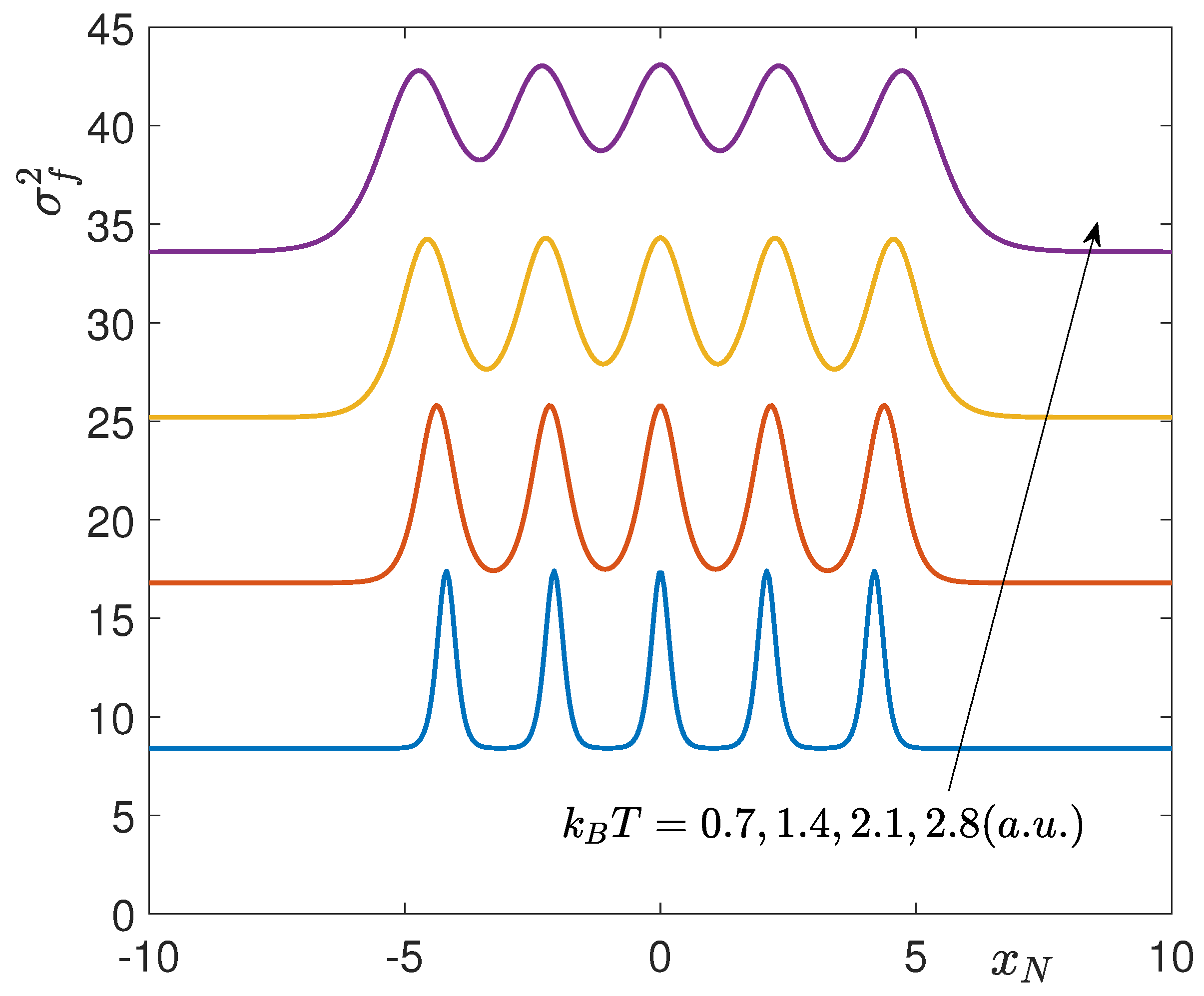
A numerical application of the results proved in this section can be found in Figure 8, Figure 9, Figure 10 and Figure 11. Similarly to the Gibbs analysis, also in this case, we observe that the kinetic part of the probability density ${\varrho }_H(\dot{f})$ is a simple Gaussian function and therefore we study in more detail the configurational density ${\varrho }_H(f;x_N)$. Coherently with this planning, in Figure 8 and Figure 9, we show the three-dimensional and the two-dimensional representation of the Helmholtz density as function of f and for a prescribed extension $x_N$. As before, the results have been obtained for four different temperatures to observe the effects of the thermal agitation on the transition processes. The parameters used in this study are the same already adopted for the Gibbs analysis, namely $N=5$, $\ell =1$ (a.u.), $k=15$ (a.u.) and $k_{B}T$ = 0.7, 1.4, 2.1, 2.8 (a.u.). We give here a description of the behavior of the system within the Helmholtz ensemble which is exactly dual with respect to the response of the Gibbs ensemble. Indeed, we observe that in spite of the saw-tooth shape of the force-extension response, the probability density of f is quite always monomodal. More precisely, it can be bimodal only with some sets of parameters and only for forces being in the transition region between two peaks of the force-extension curve. Anyway, we can affirm that this density is monomodal in the most cases of practical interest. To better explain this point, we observe that in order to obtain the probability density of f for a prescribed $x_N$, we have to section the plots in Figure 8 and Figure 9 with a plane parallel to the f-axis and, at the same time, perpendicular to the $x_N$-axis. By performing this operation, in spite of the complex shape of ${\varrho }_H(f;x_N)$, we get monomodal functions (with the exceptions discussed above). This can be observed in Figure 10, where we plotted several curves ${\varrho }_H(f;x_N)$ for different values of the prescribed extension $x_N$. As before, we remark that the knowledge of the full probability density for the Helmholtz case can be used to determine the expected values of higher order. As an example, in Figure 11 we plotted the variance of the force f, necessary to impose the extension $x_N$. Interestingly enough, the variance is an increasing function of the temperature, as expected, and shows some peaks in correspondence to the switching of state of each unit. This is coherent with the general idea that the variance of the physical quantities is larger in proximity to a phase transition. Again, we underline the dual behavior of the Gibbs and Helmholtz ensembles. Indeed, while the variance for the Gibbs case is given by a single peak corresponding to the synchronized transition of the units, for the Helmholtz ensemble we have a peak for each transition, underlying the sequential behavior of this process.

6. Discussion and Conclusions

In this work we considered the comparison of Gibbs (isotensional) and Helmholtz (isometric) ensembles of the (equilibrium) statistical mechanics in the context of the stretching of chains of bistable units. The thermodynamics of the force-extension relations leads to different responses of the two ensembles for small systems, i.e., far from the thermodynamic limit. In particular, the Gibbs response is characterized by a force plateau corresponding to the synchronized transitions of the units, whereas the Helmholtz response can be viewed as a saw-tooth curve representing the sequential transitions of the units. We remark that, when the number of units approaches infinity, the two ensembles become equivalent from the statistical point of view and, therefore, the two Gibbs and Helmholtz force-extension responses become coincident. This general picture, well known in the context of the thermodynamics of small systems, has been widely confirmed experimentally by means of the force spectroscopy methodologies (see Introduction).

From the theoretical point of view, this scenario has been complemented here by introducing a method to elaborate the full statistics of these processes at thermodynamic equilibrium, i.e., by the calculation of the probability density of the fluctuating quantities and not only of their average values. The added information is useful to draw full comparisons with experiments and to extract more statistical features valuable from the theoretical point of view. As an example, the knowledge of the complete probability density can be used to evaluate expected values of higher order such as variances, covariances and so forth. Concerning the comparison with experiments, the devices today available to observe the mechanical response of macromolecules (force spectroscopy tweezers) are very refined and allow not only for the measurement of the average values of the main quantities but also to probe the distributions of the same quantities. This can be done by collecting the information of many trajectories of the system and to extract from those data the statistical picture of the system evolution. It means that it is important to update the theoretical devices in order to be able to calculate the probability density of the fluctuating quantities in terms of the deterministic applied ones.

Within the Gibbs ensemble, we apply a deterministic force and we measure a stochastic extension. So, we developed here a method to give the probability density of this extension and its rate with respect to the time. On the other hand, within the Helmholtz ensemble, we prescribe a deterministic extension and we measure a stochastic force. Therefore, we obtained in this work the probability density of the force and its time derivative. It is interesting to observe that in both cases these probability densities can be always written in terms of a combination of the two Gibbs and Helmholtz partition functions. This is a typical outcome in statistical mechanics, where all relevant quantities are typically written by means of the partition functions. We remark that, in the case of the number of units approaching infinity, we have the ensemble equivalence as above said. It means that the force-extension curves are the same for both ensembles but the probability densities are not the same because are simply defined on different variables.

The results obtained for the specific case of a chain of bistable elements show the emergence of an intriguing duality between the two ensembles. For the isotensional condition, the force-extension curve is monotone with a characteristic force plateau and the density $\varrho (x_N;f)$ is multimodal in the transition region (near $x_N=0$ and $f=0$). Conversely, for the isometric condition, the force-extension curve is composed of a series of peaks while the density $\varrho (f;x_N)$ is simply monomodal. This duality is also reflected in the behavior of the variances of these processes. In the Gibbs ensemble we obtained a monomodal variance ${\sigma }_x^2$ with the symmetric peak at $f=0$, whereas in the Helmholtz ensemble we obtained a multimodal variance ${\sigma }_f^2$ with a peak for each transition value of $x_N$. Of course, the peaks of variance must be explained through large fluctuations characterizing the switching of the units states (classically, it is typical for the phase transitions).

To go further with this analysis, in the next future we will take into consideration the case of bistable elements with two potential wells at different equilibrium length (as considered in this paper) and different equilibrium energy (here we supposed the same energetic level for the two basins). The introduction of the energy difference $\mathsf{\Delta }E$ between the states will be useful to describe more realistic systems, such as protein domains and other macromolecules of biological origin. Another perspective concerns the consideration of the out-of-equilibrium thermodynamics useful to evaluate the dynamics (the time evolution) of the introduced probability densities, with application to the interpretation of force spectroscopy experiments. To do this, we plan to use our spin variables coupled with a first order dynamics governed by the Kramers rates, which depend on the energy barrier between the wells.

To conclude, it is important to underline that the thermodynamics of small systems and bistable-multistable systems is relevant not only for the studies concerning macromolecules and biophysics but only for several applications to nanoscience and nanotechnology, namely for the better understanding of plasticity, hysteretic behaviors and martensitic transformations in solids, micro- and nano-magnetism, ferromagnetic alloys, nano-indented substrates, bistable nanosystems for energy harvesting and transport phenomena in bistable nano-systems such as, e.g., tunnel effect transistors.

References

- Bustamante, C.; Liphardt, J.; Ritort, F. The Nonequilibrium Thermodynamics of Small Systems. Phys. Today 2005, 58, 43. [Google Scholar] [CrossRef]
- Dieterich, E.; Camunas-Soler, J.; Ribezzi-Crivellari, M.; Seifert, U.; Ritort, F. Control of force through feedback in small driven systems. Phys. Rev. E 2016, 94, 012107. [Google Scholar] [CrossRef] [PubMed]
- Winkler, R.G. Equivalence of statistical ensembles in stretching single flexible polymers. Soft Matter 2010, 6, 6183. [Google Scholar] [CrossRef]
- Manca, F.; Giordano, S.; Palla, P.L.; Zucca, R.; Cleri, F.; Colombo, L. Elasticity of flexible and semiflexible polymers with extensible bonds in the Gibbs and Helmholtz ensembles. J. Chem. Phys. 2012, 136, 154906. [Google Scholar] [CrossRef] [Green Version]
- Manca, F.; Giordano, S.; Palla, P.L.; Cleri, F.; Colombo, L. Response to “Comment on ‘Elasticity of flexible and semiflexible polymers with extensible bonds in the Gibbs and Helmholtz ensembles”’ [J. Chem. Phys. 138, 157101 (2013)]. J. Chem. Phys. 2013, 138, 157102. [Google Scholar] [CrossRef] [PubMed] [Green Version]
- Manca, F.; Giordano, S.; Palla, P.L.; Cleri, F. On the equivalence of thermodynamics ensembles for flexible polymer chains. Phys. A Stat. Mech. Its Appl. 2014, 395, 154–170. [Google Scholar] [CrossRef]
- Van Kampen, N.G. Stochastic Processes in Physics and Chemistry; Elsevier: Amsterdam, The Netherlands, 1981. [Google Scholar]
- Risken, H. The Fokker-Planck Equation; Springer: Berlin, Germany, 1989. [Google Scholar]
- Coffey, W.T.; Kalmykov, Y.P.; Waldron, J.P. The Langevin Equation; World Scientific: Singapore, 2004. [Google Scholar]
- Manca, F.; Déjardin, P.-M.; Giordano, S. Statistical mechanics of holonomic systems as a Brownian motion on smooth manifolds. Annalen der Physik 2016, 528, 381–393. [Google Scholar] [CrossRef]
- Esposito, M.; Van den Broeck, C. Three faces of the second law. I. Master equation formulation. Phys. Rev. E 2010, 82, 011143. [Google Scholar] [CrossRef]
- Van den Broeck, C.; Esposito, M. Three faces of the second law. II. Fokker-Planck formulation. Phys. Rev. E 2010, 82, 011144. [Google Scholar] [CrossRef]
- Tomé, T.; de Oliveira, M.J. Entropy production in irreversible systems described by a Fokker-Planck equation. Phys. Rev. E 2010, 82, 021120. [Google Scholar] [CrossRef]
- Tomé, T.; de Oliveira, M.J. Stochastic approach to equilibrium and nonequilibrium thermodynamics. Phys. Rev. E 2015, 91, 042140. [Google Scholar] [CrossRef]
- Jarzynski, C. Nonequilibrium Equality for Free Energy Differences. Phys. Rev. Lett. 1997, 78, 2690. [Google Scholar] [CrossRef]
- Jarzynski, C. Equilibrium free-energy differences from nonequilibrium measurements: A master-equation approach. Phys. Rev. E 1997, 56, 5018. [Google Scholar] [CrossRef]
- Crooks, G. Entropy production fluctuation theorem and the nonequilibrium work relation for free energy differences. Phys. Rev. E 1999, 60, 2721. [Google Scholar] [CrossRef]
- Collin, D.; Ritort, F.; Jarzynski, C.; Smith, S.B.; Tinoco, I.; Bustamante, C. Verification of the Crooks fluctuation theorem and recovery of RNA folding free energies. Nature 2005, 437, 231–234. [Google Scholar] [CrossRef]
- Jarzynski, C. Comparison of far-from-equilibrium work relations. Comptes Rendus Phys. 2007, 8, 495–506. [Google Scholar] [CrossRef] [Green Version]
- Seifert, U. Stochastic thermodynamics, fluctuation theorems and molecular machines. Rep. Prog. Phys. 2012, 75, 126001. [Google Scholar] [CrossRef] [Green Version]
- Esposito, M.; Harbola, U.; Mukamel, S. Nonequilibrium fluctuations, fluctuation theorems, and counting statistics in quantum systems. Rev. Mod. Phys. 2009, 81, 1665. [Google Scholar] [CrossRef]
- Sekimoto, K. Kinetic Characterization of Heat Bath and the Energetics of Thermal Ratchet Models. J. Phys. Soc. Jpn. 1997, 66, 1234. [Google Scholar] [CrossRef]
- Sekimoto, K. Stochastic Energetics; Springer: Berlin, Germany, 2010. [Google Scholar]
- Wang, Q.A. Maximum path information and the principle of least action for chaotic system. Chaos Solitons Fractals 2004, 23, 1253. [Google Scholar] [CrossRef]
- Wang, Q.A. Non-quantum uncertainty relations of stochastic dynamics. Chaos Solitons Fractals 2005, 26, 1045. [Google Scholar] [CrossRef]
- Lucia, U. Entropy generation and the Fokker–Planck equation. Physica A 2014, 393, 256. [Google Scholar] [CrossRef]
- Lucia, U.; Gervino, G. Fokker-Planck Equation and Thermodynamic System Analysis. Entropy 2015, 17, 763. [Google Scholar] [CrossRef]
- Lucia, U.; Grazzini, G.; Montrucchio, B.; Grisolia, G.; Borchiellini, R.; Gervino, G.; Castagnoli, C.; Ponzetto, A.; Silvagno, F. Constructal thermodynamics combined with infrared experiments to evaluate temperature differences in cells. Sci. Rep. 2015, 5, 11587. [Google Scholar] [CrossRef] [Green Version]
- Perez-Carrasco, R.; Sancho, J.M. Fokker-Planck approach to molecular motors. EPL 2010, 91, 60001. [Google Scholar] [CrossRef]
- Perez-Carrasco, R.; Sancho, J.M. Molecular motors in conservative and dissipative regimes. Phys. Rev. E 2011, 84, 041915. [Google Scholar] [CrossRef]
- Linke, W.A.; Granzier, H.; Kellermayer, M.S.Z. (Eds.) Mechanics of Elastic Biomolecules; Springer Science: Dordrecht, The Netherlands, 2003. [Google Scholar]
- Noy, A. (Ed.) Handbook of Molecular Force Spectroscopy; Springer Science: New York, NY, USA, 2008. [Google Scholar]
- Strick, T.R.; Dessinges, M.-N.; Charvin, G.; Dekker, N.H.; Allemand, J.-F.; Bensimon, D.; Croquette, V. Stretching of macromolecules and proteins. Rep. Prog. Phys. 2003, 66, 1–45. [Google Scholar] [CrossRef]
- Ritort, F. Single-molecule experiments in biological physics: Methods and applications. J. Phys. Condens. Matter 2006, 18, R531–R583. [Google Scholar] [CrossRef]
- Neuman, K.C.; Nagy, A. Single-molecule force spectroscopy: Optical tweezers, magnetic tweezers and atomic force microscopy. Nat. Methods 2008, 5, 491–505. [Google Scholar] [CrossRef]
- Kumar, S.; Li, M.S. Biomolecules under mechanical force. Phys. Rep. 2010, 486, 1–74. [Google Scholar] [CrossRef]
- Miller, H.; Zhou, Z.; Shepherd, J.; Wollman, A.J.M.; Leake, M.C. Single-molecule techniques in biophysics: A review of the progress in methods and applications. Rep. Prog. Phys. 2018, 81, 024601. [Google Scholar] [CrossRef]
- Yamahata, C.; Collard, D.; Legrand, B.; Takekawa, T.; Kumemura, M.; Hashiguchi, G.; Fujita, H. Silicon Nanotweezers with Subnanometer Resolution for the Micromanipulation of Biomolecules. J. Microelectromech. Syst. 2008, 17, 623–631. [Google Scholar] [CrossRef]
- Fisher, T.E.; Oberhauser, A.F.; Carrion-Vazquez, M.; Marszalek, P.E.; Fernandez, J.M. The study of protein mechanics with the atomic force microscope. Trends Biochem. Sci. 1999, 24, 379–384. [Google Scholar] [CrossRef]
- Li, H.; Oberhauser, A.F.; Fowler, S.B.; Clarke, J.; Fernandez, J.M. Atomic force microscopy reveals the mechanical design of a modular protein. Proc. Nat. Acad. Sci. USA 2000, 97, 6527. [Google Scholar] [CrossRef]
- Imparato, A.; Sbrana, F.; Vassalli, M. Reconstructing the free-energy landscape of a polyprotein by single-molecule experiments. Europhys. Lett. 2008, 82, 58006. [Google Scholar] [CrossRef] [Green Version]
- Bonin, M.; Zhu, R.; Klaue, Y.; Oberstrass, J.; Oesterschulze, E.; Nellen, W. Analysis of RNA flexibility by scanning force spectroscopy. Nucleic Acids Res. 2002, 30, e81. [Google Scholar] [CrossRef]
- Lipfert, J.; Skinner, G.M.; Keegstra, J.M.; Hensgens, T.; Jager, T.; Dulin, D.; Köber, M.; Yu, Z.; Donkers, S.P.; Chou, F.-C.; et al. Double-stranded RNA under force and torque: Similarities to and striking differences from double-stranded DNA. Proc. Natl. Acad. Sci. USA 2014, 111, 15408. [Google Scholar] [CrossRef]
- Smith, S.B.; Finzi, L.; Bustamante, C. Direct mechanical measurements of the elasticity of single DNA molecules by using magnetic beads. Science 1992, 258, 1122. [Google Scholar] [CrossRef]
- Marko, J.F.; Siggia, E.D. Stretching DNA. Macromolecules 1995, 28, 8759–8770. [Google Scholar] [CrossRef]
- Smith, S.M.; Cui, Y.; Bustamante, C. Overstretching B-DNA: The Elastic Response of Individual Double-Stranded and Single-Stranded DNA Molecules. Science 1996, 271, 795. [Google Scholar] [CrossRef]
- Chaurasiya, K.R.; Paramanathan, T.; McCauley, M.J.; Williams, M.C. Biophysical characterization of DNA binding from single molecule force measurements. Phys. Life Rev. 2010, 7, 299–341. [Google Scholar] [CrossRef] [Green Version]
- Manca, F.; Giordano, S.; Palla, P.L.; Cleri, F. Scaling Shift in Multicracked Fiber Bundles. Phys. Rev. Lett. 2014, 113, 255501. [Google Scholar] [CrossRef]
- Manca, F.; Giordano, S.; Palla, P.L.; Cleri, F. Stochastic mechanical degradation of multi-cracked fiber bundles with elastic and viscous interactions. Eur. Phys. J. E 2015, 38, 44. [Google Scholar] [CrossRef]
- Perret, G.; Lacornerie, T.; Manca, F.; Giordano, S.; Kumemura, M.; Lafitte, N.; Jalabert, L.; Tarhan, M.C.; Lartigau, E.F.; Cleri, F.; et al. Real-time mechanical characterization of DNA degradation under therapeutic X-rays and its theoretical modeling. Microsyst. Nanoeng. 2016, 2, 16062. [Google Scholar] [CrossRef] [Green Version]
- Winkler, R.G. Deformation of semiflexible chains. J. Chem. Phys. 2003, 118, 2919. [Google Scholar] [CrossRef] [Green Version]
- Manca, F.; Giordano, S.; Palla, P.L.; Cleri, F.; Colombo, L. Theory and Monte Carlo simulations for the stretching of flexible and semiflexible single polymer chains under external fields. J. Chem. Phys. 2012, 137, 244907. [Google Scholar] [CrossRef] [Green Version]
- Su, T.; Purohit, P.K. Thermomechanics of a heterogeneous fluctuating chain. J. Mech. Phys. Solids 2010, 58, 164. [Google Scholar] [CrossRef]
- Kierfeld, J.; Niamploy, O.; Sa-Yakanit, V.; Lipowsky, R. Stretching of semiflexible polymers with elastic bonds. Eur. Phys. J. E 2004, 14, 17. [Google Scholar] [CrossRef]
- Kramers, H.A. Brownian motion in a field of force and the diffusion model of chemical reactions. Physica 1940, 7, 284–304. [Google Scholar] [CrossRef]
- Dudko, O.K. Decoding the mechanical fingerprints of biomolecules. Q. Rev. Biophys. 2016, 49, 1–14. [Google Scholar] [CrossRef]
- Manca, F.; Pincet, F.; Truskinovsky, L.; Rothman, J.E.; Foret, L.; Caruel, M. SNARE machinery is optimized for ultrafast fusion. Proc. Natl. Acad. Sci. USA 2019. [Google Scholar] [CrossRef] [PubMed]
- Rief, M.; Fernandez, J.M.; Gaub, H.E. Elastically Coupled Two-Level Systems as a Model for Biopolymer Extensibility. Phys. Rev. Lett. 1998, 81, 4764. [Google Scholar] [CrossRef]
- Kreuzer, H.J.; Payne, S.H. Stretching a macromolecule in an atomic force microscope: Statistical mechanical analysis. Phys. Rev. E 2001, 63, 021906. [Google Scholar] [CrossRef] [PubMed]
- Manca, F.; Giordano, S.; Palla, P.L.; Cleri, F.; Colombo, L. Two-state theory of single-molecule stretching experiments. Phys. Rev. E 2013, 87, 032705. [Google Scholar] [CrossRef]
- Giordano, S. Helmholtz and Gibbs ensembles, thermodynamic limit and bistability in polymer lattice models. Continuum Mech. Thermodyn. 2018, 30, 459. [Google Scholar] [CrossRef]
- Bosaeus, N.; El-Sagheer, A.H.; Brown, T.; Smith, S.B.; Akerman, B.; Bustamante, C.; Nordén, B. Tension induces a base-paired overstretched DNA conformation. Proc. Natl. Acad. Sci. USA 2012, 109, 15179. [Google Scholar] [CrossRef] [PubMed]
- Wang, J.; Kouznetsova, T.B.; Boulatov, R.; Craig, S.L. Mechanical gating of a mechanochemical reaction cascade. Nat. Commun. 2016, 7, 13433. [Google Scholar] [CrossRef] [PubMed] [Green Version]
- Cocco, S.; Yan, J.; Léger, J.F.; Chatenay, D.; Marko, J.F. Overstretching and force-driven strand separation of double-helix DNA. Phys. Rev. E 2004, 70, 011910. [Google Scholar] [CrossRef]
- Cocco, S.; Marko, J.F.; Monasson, R.; Sarkar, A.; Yan, J. Slow nucleic acid unzipping kinetics from sequence-defined barriers. Eur. Phys. J. E 2003, 10, 249. [Google Scholar] [CrossRef]
- Rief, M.; Oesterhelt, F.; Heymann, B.; Gaub, H.E. Single Molecule Force Spectroscopy on Polysaccharides by Atomic Force Microscopy. Science 1997, 275, 1295. [Google Scholar] [CrossRef]
- Hanke, F.; Kreuzer, H.J. Conformational transitions in single polymer molecules modeled with a complete energy landscape: Continuous two-state model. Eur. Phys. J. E 2007, 22, 163. [Google Scholar] [CrossRef]
- Rief, M.; Gautel, M.; Oesterhelt, F.; Fernandez, J.M.; Gaub, H.E. Reversible unfolding of individual titin immunoglobulin domains by AFM. Science 1997, 276, 1109. [Google Scholar] [CrossRef]
- Staple, D.B.; Payne, S.H.; Reddin, A.L.C.; Kreuzer, H.J. Stretching and unfolding of multidomain biopolymers: A statistical mechanics theory of titin. Phys. Biol. 2009, 6, 025005. [Google Scholar] [CrossRef]
- Prados, A.; Carpio, A.; Bonilla, L.L. Sawtooth patterns in force-extension curves of biomolecules: An equilibrium-statistical-mechanics theory. Phys. Rev. E 2013, 88, 012704. [Google Scholar] [CrossRef]
- Bonilla, L.L.; Carpio, A.; Prados, A. Theory of force-extension curves for modular proteins and DNA hairpins. Phys. Rev. E 2015, 91, 052712. [Google Scholar] [CrossRef]
- De Tommasi, D.; Millardi, N.; Puglisi, G.; Saccomandi, G. An energetic model for macromolecules unfolding in stretching experiments. J. R. Soc. Interface 2013, 10, 20130651. [Google Scholar] [CrossRef]
- Makarov, D.E. A Theoretical Model for the Mechanical Unfolding of Repeat Proteins. Biophys. J. 2009, 96, 2160. [Google Scholar] [CrossRef]
- Giordano, S. Spin variable approach for the statistical mechanics of folding and unfolding chains. Soft Matter 2017, 13, 6877–6893. [Google Scholar] [CrossRef]
- Benedito, M.; Giordano, S. Thermodynamics of small systems with conformational transitions: The case of two-state freely jointed chains with extensible units. J. Chem. Phys. 2018, 149, 054901. [Google Scholar] [CrossRef]
- Benedito, M.; Giordano, S. Isotensional and isometric force-extension response of chains with bistable units and Ising interactions. Phys. Rev. E 2018, 98, 052146. [Google Scholar] [CrossRef]
- Caruel, M.; Allain, J.M.; Truskinovsky, L. Muscle as a Metamaterial Operating Near a Critical Point. Phys. Rev. Lett. 2013, 110, 248103. [Google Scholar] [CrossRef]
- Caruel, M.; Truskinovsky, L. Statistical mechanics of the Huxley-Simmons model. Phys. Rev. E 2016, 93, 062407. [Google Scholar] [CrossRef]
- Ericksen, J.L. Equilibrium of bars. J. Elast. 1975, 5, 191. [Google Scholar] [CrossRef]
- Müller, I.; Villaggio, P. A model for an elastic-plastic body. Arch. Ration. Mech. Anal. 1977, 65, 25. [Google Scholar] [CrossRef]
- Fedelich, B.; Zanzotto, G. Hysteresis in discrete systems of possibly interacting elements with a double-well energy. J. Nonlinear Sci. 1992, 2, 319–342. [Google Scholar] [CrossRef]
- Puglisi, G.; Truskinovsky, L. Thermodynamics of rate-independent plasticity. J. Mech. Phys. Sol. 2005, 53, 655. [Google Scholar] [CrossRef]
- Caruel, M.; Allain, J.-M.; Truskinovsky, L. Mechanics of collective unfolding. J. Mech. Phys. Sol. 2015, 76, 237. [Google Scholar] [CrossRef]
- Efendiev, Y.R.; Truskinovsky, L. Thermalization of a driven bi-stable FPU chain. Continuum Mech. Thermodyn. 2010, 22, 679. [Google Scholar] [CrossRef]
- Mielke, A.; Truskinovsky, L. From Discrete Visco-Elasticity to Continuum Rate-Independent Plasticity: Rigorous Results. Arch. Ration. Mech. Anal. 2012, 203, 577–619. [Google Scholar] [CrossRef]
- Benichou, I.; Givli, S. Structures undergoing discrete phase transformation. J. Mech. Phys. Sol. 2013, 61, 94. [Google Scholar] [CrossRef]
- Restrepo, D.; Mankame, N.D.; Zavattieri, P.D. Phase transforming cellular materials. Extr. Mech. Lett. 2015, 4, 52–60. [Google Scholar] [CrossRef] [Green Version]
- Frazier, M.J.; Kochmann, D.M. Band gap transmission in periodic bistable mechanical systems. J. Sound. Vib. 2017, 388, 315–326. [Google Scholar] [CrossRef]
- Katz, S.; Givli, S. Solitary waves in a bistable lattice. Extr. Mech. Lett. 2018, 22, 106–111. [Google Scholar] [CrossRef]
- Hwang, M.; Arrieta, A.F. Nonlinear dynamics of bistable lattices with defects. In Proceedings of the SPIE, Health Monitoring of Structural and Biological Systems, Portland, OR, USA, 25–29 March 2017; Volume 101701A. [Google Scholar] [CrossRef]
- Hwang, M.; Arrieta, A.F. Response invariance in a lattice of bistable elements with elastic interactions. In Proceedings of the SPIE 10595, Active and Passive Smart Structures and Integrated Systems XII, Denver, CO, USA, 4–8 March 2018; Volume 105950X. [Google Scholar] [CrossRef]
- Harne, R.L.; Schoemaker, M.E.; Wang, K.W. Multistable chain for ocean wave vibration energy harvesting. In Proceedings of the SPIE 9057, Active and Passive Smart Structures and Integrated Systems, San Diego, CA, USA, 9–13 March 2014; Volume 90570B. [Google Scholar] [CrossRef]
Figure 1.
Bistable symmetric potential energy of a single domain (blue dashed line) and its approximation by means of four parabolic profiles (red solid lines).
Figure 2.
Average force-extension curves and average spin variables (plotted by means of dimensionless quantities) for the Gibbs ensemble with and = 10, 15, 30, 100.
Figure 3.
Average force-extension curves and average spin variables (plotted by means of dimensionless quantities) for the Helmholtz ensemble with and = 10, 15, 30, 100.
Figure 4.
Three-dimensional representation of the Gibbs density (see Equation (33)) obtained with , (a.u.), (a.u.) and = 0.7, 1.4, 2.1, 2.8 (a.u.).
Figure 5.
Two-dimensional representation of the Gibbs density (see Equation (33)) obtained with , (a.u.), (a.u.) and = 0.7, 1.4, 2.1, 2.8 (a.u.).
Figure 6.
Examples of multimodal curves obtained through the Gibbs density (see Equation (33)). On the left panel, the two-dimensional representation of the Gibbs density is shown with the cuts corresponding to the curves plotted on the right panel. We used , (a.u.), (a.u.), = 1 (a.u.) and different values of the applied force f, as indicated in the legend.
Figure 7.
Variance of obtained by the Gibbs density . As before, we used , (a.u.), (a.u.) and = 0.7, 1.4, 2.1, 2.8 (a.u.).
Figure 8.
Three-dimensional representation of the Helmholtz density (see Equation (54)) obtained with , (a.u.), (a.u.) and = 0.7, 1.4, 2.1, 2.8 (a.u.).
Figure 9.
Two-dimensional representation of the Helmholtz density (see Equation (54)) obtained with , (a.u.), (a.u.) and = 0.7, 1.4, 2.1, 2.8 (a.u.).
Figure 10.
Examples of monomodal curves obtained through the Helmholtz density (see Equation (54)). On the left panel, the two-dimensional representation of the Helmholtz density is shown with the cuts corresponding to the curves plotted on the right panel. We used , (a.u.), (a.u.), = 1 (a.u.) and different values of the prescribed position , as indicated in the legend.
Figure 11.
Variance of f obtained by the Helmholtz density . As before, we used , (a.u.), (a.u.) and = 0.7, 1.4, 2.1, 2.8 (a.u.).
© 2019 by the authors. Licensee MDPI, Basel, Switzerland. This article is an open access article distributed under the terms and conditions of the Creative Commons Attribution (CC BY) license (http://creativecommons.org/licenses/by/4.0/).
Share and Cite
MDPI and ACS Style
Benedito, M.; Manca, F.; Giordano, S. Full Statistics of Conjugated Thermodynamic Ensembles in Chains of Bistable Units. Inventions 2019, 4, 19. https://doi.org/10.3390/inventions4010019
AMA Style
Benedito M, Manca F, Giordano S. Full Statistics of Conjugated Thermodynamic Ensembles in Chains of Bistable Units. Inventions. 2019; 4(1):19. https://doi.org/10.3390/inventions4010019
Chicago/Turabian StyleBenedito, Manon, Fabio Manca, and Stefano Giordano. 2019. "Full Statistics of Conjugated Thermodynamic Ensembles in Chains of Bistable Units" Inventions 4, no. 1: 19. https://doi.org/10.3390/inventions4010019