Application of Various Price-Discount Policy for Deteriorated Products and Delay-in-Payments in an Advanced Inventory Model


1
Department of Mathematics, Government General Degree College, Gopiballavpur-II, Beliaberah, Jhargram, West Bengal 721517, India
2
Department of Industrial Engineering, Yonsei University, 50 Yonsei-ro, Sinchon-dong, Seadaemun-gu, Seoul 03722, Korea
3
Department of Mathematics, Kazi Nazrul University, Asansol, West Bengal 713340, India
*
Author to whom correspondence should be addressed.
Inventions 2020, 5(3), 50; https://doi.org/10.3390/inventions5030050
Submission received: 8 August 2020
/
Revised: 15 September 2020
/
Accepted: 16 September 2020
/
Published: 20 September 2020
(This article belongs to the Section Inventions and Innovation in Design, Modeling and Computing Methods)
Abstract
:In this proposed research, clear prospects of a real life marketing scenario, by analyzing a price discount policy and variable demand, are derived. The proposed study presents a production model along with time-dependent and selling price related demand for decaying items. Items deteriorate over time, therefore, considering deterioration in this model makes it more acceptable to the present marketing situation. The concept of delay-in-payments is utilized in this inventory system. In this research, a retailer buys some products, enjoys constant credit-period offers which are provided by the supplier. This model depicts a price discount strategy which is based on purchasing cost to attract more consumers in any business industry. By using this strategy, any manufacturer or business may gain more profit in comparison to methods suggested by earlier literature. The average profit function of the inventory system is maximized analytically and also finds the selling-price per unit and duration of the inventory cycle optimally. A numerical example, along with a case study and their graphical representations, are incorporated to verify the optimality of this research very clearly. The findings of this research have maximized the average profit function more than the existing literature.
1. Introduction
Deterioration of items is one of the major problems to be considered in the manufacturing industry. In a practical life situation, it is too hard to maintain the deterioration of products such as fruits and vegetables. These types of products, which deteriorate over time, are not in good enough condition to fulfill the customers demand. Therefore, the effect of deterioration cannot be disregarded in production lot-size. Dave and Pandya [1] presented two separate inventory models, that is, one was an infinite finite horizon model, the other was a finite horizon model with deteriorated items. Bhunia et al. [2] discovered an inventory system for decayed items from two different warehouses with preserving technologies. Partially backlogged shortages were considered as waiting time related. Different realistic cases, sub cases, and scenarios corresponding problems were considered as non-linear constrained optimization problems. By mentioning the rate of deterioration as controllable variables, an inventory system in a novel freshness-preservation effort (FPE) indicator was demonstrated by Yang et al. [3]. They observed the optimal values of the FPE indicator and with that the optimal order quantity was also examined. After that, Khakzad and Gholamian [4] obtained an inventory system for decaying products regarding the impact of inspection times. They mentioned the inspection times throughout the replenishment duration. They also assumed that the supplier was going to inflict some payments in an advance policy on the retailer. Their study depicted that the average decaying rate was related to the inspections number during every period.
Another important factor in an inventory system is the time. Whenever any business launches their branded new product, it is observed that the demand graph of that item is not always continuous over time. The demand graph of that product is constant within a couple of times but not always. After that, as time passes, demand for that product may increase or may gradually decrease. Due to the ups and downs nature of that demand graph, it is better to consider demand as time dependent. Hsu and Li [5] surveyed a mathematical programming model which was non-linear for optimizing the delivery process with time related demand. Their results proved that discriminating service policy was a more beneficial technique with respect to uniform strategy. Khanra et al. [6] examined an inventory system with quadratic demand with respect to time. The concept of delay-in-payments was used in their model. Shortages were considered after some variable time. In this direction of research, Wang et al. [7] showed a mixed-integer programming system while the demand was a function of time. Their model assumed the train capacity. They minimized the passenger total waiting duration along with the amount of passengers unable to transfer. Their study considered Genetic Algorithm (GA) and Grey Wolf Optimizer (GWO) for determining the model. Afterwards, Chen et al. [8] represented a decaying inventory system for variable demand in a multi-period finite horizon. They described several demand patterns such as constant, time-dependent, selling price-dependent, and stock-dependent.
Pricing is a major factor in the success of a business. Like time, demand of products may be affected by the selling price. Selling price plays a vital role in every business association. As much as the selling price of an item decreases, the demand graph of that product increases. For the other case, where the selling price of any products gradually increases, the demand graph becomes low. Therefore, selling price has significant value in an inventory system. Krugon and Nagaraju [9] established a two-echelon inventory model in which non-linear price dependent demand was assumed along with the credit period. A sustainable integrated inventory system was formulated by Dey et al. [10] to reduce discrete setup cost for price dependent demand. In their model, poisson distributed lead time demand was considered. Modak and Kelle [11] established a dual-channel inventory model for price and variable demand. Later, a decentralized channel optimization model was developed by Gholami et al. [12]. They modeled their study by taking into account that demand was measured as a function of pricing history. There were two price-adjusting factors in a bi-level (Stackelberg) model in which uncertain demand patterns were described for perishable items. In their stochastic demand model, to describe an uncertain demand pattern, they highlighted price-dependent memory functions. By focusing the demand as selling price related, Torkaman et al. [13] discovered a production-routing model with the classification of various demand functions. Demand was assumed as a continuous diminishing function of selling price. Their study consists of two Outer Approximation (OA) grounded algorithms.
Every e-commerce business industry or any other industrial enterprize is always concerned about their profit level. They often provide some discount policy to attract more consumers as much as they can. For this phenomenon, customers are much more willing to buy products from marketing companies. As a result, those companies are able to achieve higher profit value. Alfares and Ghaithan [14] developed an inventory system by assuming demand rate which was variable and holding cost that was time-dependent. Buratto [15] studied a supply chain in which two mechanisms were discussed with a cooperative advertising policy and another was a price discount technique. Jadidi et al. [16] designed a one period inventory model where a supplier offered some discount policies to the buyer. They also added demand of products which were stochastic and selling price-dependent. Li et al. [17] surveyed two-period models for obtaining a platform’s price-discount policy. Their model mainly consists of three several online coupon redemption policies. These policies were—the first one, described as a platform, provides one short-term coupon in period 1 and customers can only redeem that coupon in period 1. For the second coupon policy, customers can only redeem the coupon in period 2. For the third coupon policy, the platform recommended two coupons, that is, a short-term as well as a long-term coupon in period 1, and customers can redeem only one coupon in every period. Further, Qiu and Lee [18] designed a rail transport pricing model with some quantity discount policy for a dry port system. In their model, they enhanced the dry port’s profit by utilizing the concept of a single breakpoint pricing strategy. They also considered the Stackelberg game approach to solve their model under the single breakpoint pricing scheme.
The trade-credit period is generally defined as the constant time-period provided by the supplier to retailers for adjusting their payment. In that time-period, retailers are not charged to pay any type of interest. After that particular time-period, some interest is charged to the retailer along with their due payment. In addition, the retailer allows their consumer a trade-credit duration which is partial. Interest is charged to consumers if they are not able to settle the purchasing amount. For this reason, the retailer can postpone their due payment until the last moment of a given duration. Hence, the retailer can gain more profits. Li et al. [19] generated an inventory model where the retailer’s due payments was allowed by the supplier. They incorporated a corresponding inventory game for delay-in-payments, and showed that its core was nonempty. Their model generated a core allocation rule that can be reached through a population monotonic allocation scheme. Zou and Tian [20] formulated a supply chain model for developing a trade-credit matter. They also depicted some payment and ordering techniques. Aljazzar et al. [21] derived a supply chain model by designing the idea of delays-in-payments. Their model presented environmental as well as economic execution of a supply chain model. They also described the transportation cost along with the carbon emissions cost. Optimizing results in their model showed that adopting delay-in-payments policy improved both environmental as well as the economic execution of the supply chain model. Later, Jory et al. [22] examined the connection between trade-credit and its significance value for U.S. public firms with government economic policy uncertainty (EPU). They portrayed the effect of how the trade-credit strategy changed on firm value. They also observed that fastening trade-credit throughout periods of high economic policy uncertainty enhanced shareholder value only to a certain level.
It is observed that each of the above parameters has its own impact in any manufacturing companies for enhancing their profit value. Therefore, it is necessary to incorporate each of those parameters in any advanced inventory model. This model is established with the goal of improving the benefit level of production companies. For this phenomenon, a production model is developed in which the average profit function of supplier-retailer inventory system is to be maximized. This study extended earlier research by inserting some price discount technique, variable demand, consideration of deterioration of products, trade-credit policy, and finite replenishment rate. This model determines a practical approach to raise a higher profit level in comparison to earlier research studies. The obtained result in this proposed study would help to improve the profit level in every business organization.
Contribution of this Research
This research is mainly formulated on the basis of some factors. These factors are as follows—the first factor is to increase the growth of the profitability level of any business organization. To fulfill this factor of this research, some essential policies are inserted that are defined as delay-in-payments technique and a price-discount policy. The thought behind this idea of the delay-in-payments technique is that by using this policy any industry sector will be benefitted by earning some interest. That price-discount policy is primarily included in this research to attract the attention of consumers.
The second factor is to develop this model more acceptable in the present scenario by incorporating the realistic assumptions, that is, deterioration while considering any products with their shelf life. Because it is obvious that none of the products remain in a good condition over the whole time within their shelf life. These products deteriorate during the changes of time interval. For this reason, this research did not neglect the important assumption of deterioration. The consideration of deterioration constructed in this study is even more fruitful in comparison to the other research that does not include deterioration.
The third factor is to extend this research by adding some other realistic parameters which are variable demand, trade-credit strategy, and finite replenishment rate.
By analyzing all these key parameters, this study built a better profit level compared with previous research. With the help of these factors, one by one, this research contributes to any marketing agencies to achieve their goal of enriching the optimum values of the profit function.
2. Literature Review
Products deteriorate over time. Therefore, the quality of deteriorated products decrease automatically. Hence, these products are not in a good condition to sell in the market. For this matter, companies are not able to fulfil customer demand. Thus, the affect of deterioration cannot be discarded in production factories. Heng et al. [23] derived the effect of decay in an inventory model. Skouri and Papachristos [24] depicted an inventory model by highlighting deterioration, variable shortage, and opportunity cost. Further, Sarkar et al. [25] described a study regarding two ways trade-credit policy. They mentioned that deterioration was measured as time dependent in their model. Later, Sarkar et al. [26] minimized the total setup cost and raised the item’s quality for deteriorating products. Iqbal and Sarkar [27] incorporated preservation technology for deteriorated items in an integrated inventory model.
In traditional studies, the demand rate was measured as a constant over whole time. That assumption for constant demand is not true as the demand of any product may fluctuate over time. Some notable research models about linear-trend demand were created by many researchers. Goswami and Chaudhuri [28] explained the inventory replenishment technology for a deteriorating item. By introducing the concept of exponentially deteriorating items, Hariga [29] proposed two distinct efficient solution procedures to develop optimal replenishment schedules for decayed items whose lifetime was fixed and variable demand. Li [30] studied the delivery method of a distributor by spotlighting carbon-emissions and retailers’ variable demand. Zhao et al. [31] described a multi layered stages inventory system with the fact that was the time-dependent demand.
Most of the products are available in the market, where the rate of demand of products and selling-price are closely related. Whenever the price of any product reduces, customers are more affective to that product, that is, demand of that product increases directly. Avinadav et al. [32] discussed a study related to perishable products in an inventory system for several demand patterns. Sarkar and Saren [33] obtained the ordering and transferring policy with several demand functions for deteriorating items. These items were transferred by using a multi-delivery policy with equal delivery lot-size. Demand was taken to be as time, time-price, price and exponentially time dependent. Sarkar et al. [34] depicted the concept that demand was credit period related and selling price related. They extended their research by adding time dependent deteriorating items. By considering demand as quality dependent and selling price, Dey et al. [35] incorporated the autonomation policy to classify defective products. Khanna et al. [36] generated the inventory model with defective products and selling price-dependent demand.
In general, several companies provide some price-discount to consumers if they purchase a bulk size of inventories. For this reason, companies can gain more demand of items and increase their profit level. At the same time, for selling a large amount of inventories, companies can minimize the holding cost of stocks. Xu et al. [37] represented the effect of price discount policy and trade-ins. A “low” substitutability level in their model stated that trade-ins were lower. Sheehan et al. [38] highlighted the impact of the price discount’s magnitude on customer purchase intentions at the time of online shopping. Hota et al. [39] described a supply chain with the impact of unreliable players, backorder price discounts, and service-dependent demand. They also considered an investment function for reducing the lead time crashing cost (LTCC).
Earlier, it was assumed that retailers pay instantly for the products they purchase from a supplier. Nowadays, the supplier provides a constant time to retailer for adjusting the remaining purchasing cost. This constant period of time is known as the trade-credit period. Nowadays, retailers also offer a trade-credit procedure to consumers for gaining maximum profit. The view-point of credit-connected demand and trade-credit method was introduced by Jaggi et al. [40] to reflect the present-life situations. Sarkar et al. [41] considered the business policy in which suppliers provide a credit-period to customers. By inserting a cash flow technique, Mishra et al. [42] included a deteriorating inventory system with variable demand. The trade-credit technique on re-manufactured products was depicted along with time value for money. Later, Taleizadeh et al. [43] formulated a manufacturing model with defective quantities and a delayed payment system. They developed this manufacturing system to produce multi-products. See Table 1 for various research knowledge from distinct authors.
In this study, the authors extended the research of Sana and Chaudhuri [48] for deteriorated items with different functions of demand and the rate of replenishment being finite. Demand for commodities is a function of price and time. The supplier allows a constant duration of time for the retailer to pay the buying amount. In addition, the supplier provides a price-discount strategy for the buying amount to the retailer. The profit function of the retailer is maximized for a finite production rate by determining the selling-price per unit and the duration of the inventory cycle. Section 3 elucidates the mathematical model of this study. Section 4 portrays the solution methodology of this study. In Section 5, a numerical example along with a case study are designed to verify the optimality of this research clearly. In Section 6, sensitivity analysis of parameters with proper discussions are given. Section 7 depicts the managerial insights of this research. In Section 8, some concluding remarks as well as future directions are presented.
3. Mathematical Model
In this model, the same assumptions as in Sana and Chaudhuri [48] are considered except for the demand, deterioration, and finite production rate.
- In this study, the demand rate is variable. This model depicts that the demand rate of any product is affected by several parameters, for instance, time and selling price. The demand rate of products may change regarding time (Hsu and Li [5], Sarkar et al. [45]). In addition, the product’s demand rate generally enhances if the selling price of that product diminishes (Krugon and Nagaraju [9], Khanna et al. [36], Sarkar et al. [52]). For this reason, the demand of products is measured as time and price dependent. This model considers that demand increases quadratically with time and decreases linearly with selling-price.
- Delay-in-payments is highlighted in this model. Instead of allowing a single credit period, supplier permits different credit periods to the retailer for adjusting due payment (Mishra et al. [42]).
- Several price discount policies on purchasing cost are assumed in this model. As the supplier provides three credit periods to the retailer, the supplier offers a distinct price discount to the retailer in each credit period. In the first credit period, the supplier offers the biggest price discount on the purchasing cost. After that, in the second credit period the supplier offers a lesser price discount to the retailer. In the third and final credit period, no price discount is allotted for the retailer. The supplier generally utilizes this price discount technique to attract more retailers to earn maximum profit (Xu et al. [37], Sheehan et al. [38], Sana and Chaudhuri [48]).
- The production rate is finite with an infinite time horizon. Shortage and backlogging are not permitted. This model considers no lead time.
The inventory cycle starts from zero. The production rate continues until time and at to adjust the market’s demand. For adjusting the due amount, the supplier offers several credit-periods to the retailer. The buying cost at several credit-durations is
where ’s are the ith allowable delay-period at while retailer’s discount rate is .
Considering this technique, there are two cases:
Case 1
(The above condition is briefly shown in Figure 1).
Case 2
(See Figure 2).
Now, the governing differential equations for this research under the presence of deterioration are
and
From these two governing differential equations, it can be found that
where, .
and
where .
See Appendix A for values of and .
The continuity condition provides ,
Case 1
Then the carrying cost admitting charges of interest are
The profit earns credit-balance during delayed time interval [] is
The charge of interest for financing inventory throughout [] is
Therefore, the total profit is
From Equation (1), the average profit for Case 1 is
Case 2 When () The carrying cost omitting interest rates is
The profit gains throughout the delay-period [] is
Thus, the total profit is
From Equation (3), the average profit for Case 2 is
4. Solution Methodology
In this model, a classical optimization technique is applied to obtain the optimal values for the system’s average profit and when . The optimality of system’s average profit and are determined by the help of Hessian matrix. The concavity of and are obtained for inventory cycle’s duration T and selling price P by assuming second order derivatives and by checking the globally maximum condition.
The Hessian matrix for is H as follows
The necessary condition of the optimal solution is the first order partial derivatives of with respect to the inventory cycle’s duration T and selling price P are equating to zero.
that is, and .
Now,
Now, will be determined from that is, from . where,
Similarly for second decision variable which is selling price P,
By obtaining , will be observed as
The sufficient consideration for the optimum solution of is two leading principal minors are alternative in sign, that is, if the leading principal minors and at the optimal point, then H is negative definite and the function is strictly concave.
For this case, the partial derivatives of average profit function are
and
The Hessian matrix for is H as follows
The necessary condition of the optimal solution is the first order partial derivatives of with respect to inventory cycle’s duration T and selling price P are equating to zero. that is, and . Now,
Now, will be obtained from that is, from . where,
Now, for the second decision variable, that is, selling price P,
By determining , will be found as
Therefore, the sufficient condition for the optimum solution of are two leading principal minors are opposite in sign that means the leading principal minors and at the optimal point, then H is negative definite and the function is strictly concave.
For this case, partial derivatives of average profit function are
and
As the above mentioned average profit functions given by Equations (2) and (4) of the system are not linear equations and all the partial derivatives of second order of and while for both and are extremely complicated. Hence the closed form solution cannot be determined. However, by means of empirical methodologies, one can observe that the above equations are concave for lower values of and . Due to highly non-linearity of the principal minors, the optimality of the analytical method cannot be shown. The optimality of the system’s average profit and when is demonstrated numerically in the numerical example section.
5. Numerical Example
By applying the best fitted numerical data from Sana and Chaudhuri [48] model, the average profit of the system, selling-price per unit, and duration of inventory cycle are calculated.
Example 1.
Let per order, , unit/month, months, months, months, , , , , , , , unit, $/month, $/month, and units/month.
Then the optimal solutions are , months, and /unit}, , months, and /unit}, , months, and /unit}, , months, and /unit}, , months, and /unit}, , months, and /unit}.
Among the all optimal solutions, the better optimal solutions are , months, and /unit}. In Sana and Chaudhuri [48] model, the optimal solutions were , months, and /unit}. If these two optimal solutions are compared to each other, then it is obvious that this proposed model maximized more profit from the inventory system in comparison to Sana and Chaudhuri [48] model (See Figure 3).
Figure 4 indicates the average profit is globally maximum for months, and /unit. Figure 5 shows the average profit is globally maximum for months, and /unit. Figure 6 provided the average profit is globally maximum for months, and /unit. Figure 7 indicates the average profit is globally maximum for months, and /unit. Figure 8 shows that the average profit is globally maximum for months, and /unit. Figure 9 describes that the average profit is globally maximum for months, and /unit.
For , Hessian matrix H’s leading principal minors are and for optimal results of inventory cycle’s duration T and selling-price P. Hence, Hessian matrix H for is negative definite also is strictly concave.
For , Hessian matrix H’s leading principal minors are and for optimal results of inventory cycle’s duration T and selling-price P. Hence, Hessian matrix H for is negative definite also is strictly concave.
For , Hessian matrix H’s leading principal minors are and for optimal results of inventory cycle’s duration T and selling-price P. Hence, Hessian matrix H for is negative definite also is strictly concave.
For , Hessian matrix H’s leading principal minors are and for optimal results of inventory cycle’s duration T and selling-price P. Hence, Hessian matrix H for is negative definite also is strictly concave.
For , Hessian matrix H’s leading principal minors are and for optimal results of inventory cycle’s duration T and selling-price P. Hence, Hessian matrix H for is negative definite also is strictly concave.
For , Hessian matrix H’s leading principal minors are and for optimal results of inventory cycle’s duration T and selling-price P. Hence, Hessian matrix H for is negative definite also is strictly concave.
6. Sensitivity Analysis
This section highlights the impact on the system’s average profit, that is, and , while there is some deviation in various parameters , , , and (See Table 2).
- For , which is the retailer’s carrying cost, it can be seen that whenever the parameter enhances, under various circumstances the system’s average profit functions are and , where decreases.
- If the unit ordering cost increased, then the system’s average profit, that is, and , diminish rapidly. With this observation, it can be found that the variation in both positive percentage changes along with negative percentage changes are quite equal for system’s average profit, that is, and , .
- As the retailer’s interest rate gaining for credit-balances which is increases, the system’s average profit which are and where raises automatically. That means the retailers may increase their benefit level as much as they can to gain more interest. is the key parameter to increase the system’s profitability.
- The parameter which is defined as the retailer’s interest rate for financing inventory which means that the retailer has to pay that much interest to the supplier. For this parameter , it is clearly observed from the sensitivity table that system’s average profit, that is, and , when always decreases whenever the parameter changes from a negative percentage to a positive percentage.
All the impact of variations for changes of distinct parameters on system’s average profit and where are demonstrated in Figure 10, Figure 11, Figure 12, Figure 13, Figure 14 and Figure 15, respectively.
Case Study
This model discussed the concept of delaying the payments of the retailer and several pricing discount policy on purchasing cost to the retailer allowed by supplier. Any marketing companies are a practical example of this model. They offer both a delay-in-payments policy and several discount strategies to customers for increasing their sales of products. For example, the supplier offers 30 days to the retailer for settling payment. If the retailer is unable to pay the amount within 5 days, then the supplier will provide 20% discount on purchasing cost to the retailer. In the case the retailer takes 15 days to pay that amount, then the supplier will provide 10% discount on purchasing cost. Additionally after 15 days, supplier will not provide any price discount on purchasing cost to the retailer.
Based on this above case study, a numerical example is discussed which is as follows:
Let per order, , unit/month, months, , , , , , unit, $/month, $/month, and units/month.
Then the optimal solutions are , months, and /unit}, , months, and /unit}, , months, and /unit}, , months, and /unit}, , months, and /unit}, and , months, and /unit}.
Average profit function is globally maximum when months, and /unit in Figure 16. Average profit function is globally maximum when months, and /unit in Figure 17. Average profit function is globally maximum when months, and /unit in Figure 18. Average profit function is globally maximum when months, and /unit in Figure 19. Average profit function is globally maximum when months, and /unit in Figure 20. Average profit function is globally maximum when months, and /unit in Figure 21.
7. Managerial Insights
This model presented a better optimal profit which would serve the manufacturing company to obtain the benefit at the level of optimality. There are various components in this model those are responsible to increase the profit level of any industry sector. Those components are price discount strategy and delay-in-payments. By providing price discount scheme, managers are easily can attract the attention of their consumers.
1. Furthermore, delay-in-payments also act as an affecting parameter to enrich the profit matter for managers. They often allow this delay-in-payments system to their customers. For this scheme, managers are much more capable of enhancing their profit level which is the basic business concern in any companies.
2. Sensitivity analysis of this research is also portrays the same matter of how the rate of interest gain for any inventory system is the primary factor to achieve higher profit margin. This study serves the managers to highlight their average profit by evaluating inventory cycle’s duration and selling-price practically.
8. Conclusions
An inventory model was extended from the extension of Sana and Chaudhuri’s [48] model. Using the concept of model of Sana and Chaudhuri [48], the supplier offers several discount systems to the retailer for stimulating their business. This study generated a production model with deterioration for time-dependent as well as selling-price-related demand. Deterioration is also considered in this study. In this model, the optimal results of selling-price and the inventory cycle’s length for better optimality of an average profit function of the inventory system are calculated briefly. At the end of the numerical example, a comparison is done with the optimal findings of the Sana and Chaudhuri [48] model. This model enhances higher profit for the inventory system more than previous literature. Further, this work can be expanded to a multi-item inventory model (Tamjidzad and Mirmohammadi [53], Tayyab et al. [54]) with probabilistic demand (Khosravikia and Clayton [55], Guo et al. [56]), machine breakdown (Peymankar et al. [57], Chiu et al. [58]), imperfect production (Sarkar and Saren [59], Sarkar et al. [60]) and solving by any meta-heuristic procedure (Vahdani et al. [61]).
Author Contributions
Conceptualization, B.S.; Methodology, S.S. and R.K.B.; Software, S.S.; Validation, B.S.; Formal analysis, R.K.B.; Investigation, B.S.; Resources, S.S. and R.K.B.; Data curation, B.S. and S.S.; Writing—original draft preparation, R.K.B. and S.S.; writing—review and editing, S.S.; Visualization, B.S. and R.K.B.; Supervision, B.S. All authors have read and agreed to the published version of the manuscript.
Funding
This study received no external funding.
Conflicts of Interest
No conflict of interest declared by the authors.
Appendix A
Appendix B
Decision Variables
| P | selling-price ($/unit) |
| T | inventory cycle’s length (months) |
Parameters
| inventory’s level throughout the time interval (units) | |
| inventory’s level throughout (units) | |
| production rate (unit/unit time) | |
| K | delay-period (unit time) |
| allowable delay-duration (unit time) | |
| demand is related to both price, time, , , and all are scaling parameters. | |
| decaying rate, | |
| rate of discount on MRP at the ith allowable delay-period (%) | |
| cost of purchasing ($/unit) | |
| maximum retail price (MRP) ($/unit) | |
| carrying cost ($/unit) | |
| ordering cost ($/order) | |
| interest rate gaining for credit-balance (/$/unit time) | |
| interest rate for financing inventory (/$/unit time) | |
| production time | |
| optimal inventory cycle’s length (months) | |
| optimal selling-price ($/unit) | |
| average profit function when ($) | |
| system’s average profit during ($) |
References
- Dave, U.; Pandya, B. Inventory returns and special sales in a lot-size system with constant rate of deterioration. Eur. J. Oper. Res. 1985, 19, 305–312. [Google Scholar] [CrossRef]
- Bhunia, A.K.; Jaggi, C.K.; Sharma, A.; Sharma, R. A two-warehouse inventory model for deteriorating items under permissible delay in payment with partial backlogging. Appl. Math. Comput. 2014, 232, 1125–1137. [Google Scholar] [CrossRef]
- Yang, Y.; Chi, H.; Zhou, W.; Fan, T.; Piramuthu, S. Deterioration control decision support for perishable inventory management. Decis. Support Syst. 2020, 134, 113308. [Google Scholar] [CrossRef]
- Khakzad, A.; Gholamian, M.R. The effect of inspection on deterioration rate: An inventory model for deteriorating items with advanced payment. J. Clean. Prod. 2020, 254, 120117. [Google Scholar] [CrossRef]
- Hsu, C.I.; Li, H.C. Optimal delivery service strategy for internet shopping with time-dependent consumer demand. Trans. Res. Part E Logis. Trans. Rev. 2006, 42, 473–497. [Google Scholar] [CrossRef]
- Khanra, S.; Mandal, B.; Sarkar, B. An inventory model with time dependent demand and shortages under trade credit policy. Econ. Model. 2013, 35, 349–355. [Google Scholar] [CrossRef]
- Wang, Y.; Li, D.; Cao, Z. Integrated timetable synchronization optimization with capacity constraint under time-dependent demand for a rail transit. Comput. Ind. Eng. 2020, 142, 106374. [Google Scholar] [CrossRef]
- Chen, L.; Chen, X.; Keblis, M.F.; Li, G. Optimal pricing and replenishment policy for deteriorating inventory under stock-level-dependent, time-varying and price-dependent demand. Comput. Ind. Eng. 2019, 135, 1294–1299. [Google Scholar] [CrossRef]
- Krugon, S.; Nagaraju, D. Optimality of cycle time and inventory decisions in a two echelon inventory system with non linear price dependent demand under credit period. Mater. Today Proc. 2018, 5, 12499–12508. [Google Scholar] [CrossRef]
- Dey, B.K.; Sarkar, B.; Sarkar, M.; Pareek, S. An integrated inventory model involving discrete setup cost reduction, variable safety factor, selling-price dependent demand, and investment. RAIRO Oper. Res. 2019, 53, 39–57. [Google Scholar] [CrossRef] [Green Version]
- Modak, N.M.; Kelle, P. Managing a dual-channel supply chain under price and delivery-time dependent stochastic demand. Eur. J. Oper. Res. 2019, 272, 147–161. [Google Scholar] [CrossRef]
- Gholami, R.A.; Sandal, L.K.; Ubøe, J. A solution algorithm for multi-period bi-level channel optimization with dynamic price-dependent stochastic demand. Omega 2020. [Google Scholar] [CrossRef]
- Torkaman, S.; Jokar, M.R.A.; Mutlu, N.; Woensel, T.V. Solving a production-routing problem with price-dependent demand using an outer approximation method. Comput. Ind. Eng. 2020, 123, 105019. [Google Scholar] [CrossRef]
- Alfares, H.K.; Ghaithan, A.M. Inventory and pricing model with price-dependent demand, time-varying holding cost, and quantity discounts. J. Comput. Ind. Eng. 2016, 94, 170–177. [Google Scholar] [CrossRef]
- Buratto, A.; Cesaretto, R.; Giovanni, P.D. Consignment contracts with cooperative programs and price discount mechanisms in a dynamic supply chain. Int. J. Prod. Econ. 2019, 218, 72–82. [Google Scholar] [CrossRef]
- Jadidi, O.; Jaber, M.Y.; Zolfaghari, S. Joint pricing and inventory problem with price dependent stochastic demand and price discounts. Comput. Ind. Eng. 2017, 114, 45–53. [Google Scholar] [CrossRef]
- Li, C.; Chu, M.; Zhou, C.; Zhao, L. Two-period discount pricing strategies for an e-commerce platform with strategic consumers. Comput. Indu. Eng. 2020, 147, 106640. [Google Scholar] [CrossRef]
- Qiu, X.; Lee, C.Y. Quantity discount pricing for rail transport in a dry port system. Trans. Res. Part E Logis. Trans. Rev. 2019, 122, 563–580. [Google Scholar] [CrossRef]
- Li, J.; Feng, H.; Zeng, Y. Inventory games with permissible delay in payments. Eur. J. Oper. Res. 2015, 234, 694–700. [Google Scholar] [CrossRef]
- Zou, X.; Tian, B. Retailer’s optimal ordering and payment strategy under two-level and flexible two-part trade credit policy. Comput. Ind. Eng. 2020, 142, 106317. [Google Scholar] [CrossRef]
- Aljazzar, S.M.; Gurtu, A.; Jaber, M.Y. Delay-in-payments—A strategy to reduce carbon emissions from supply chains. J. Clean. Prod. 2018, 170, 636–644. [Google Scholar] [CrossRef]
- Jory, S.R.; Khieu, H.D.; Ngo, T.N.; Phan, H.V. The influence of economic policy uncertainty on corporate trade credit and firm value. J. Corps Financ. 2020, 64, 101671. [Google Scholar] [CrossRef]
- Heng, K.J.; Labban, J.; Linn, R.J. An order-level lot-size inventory model for deteriorating items with finite replenishment rate. Comput. Ind. Eng. 1991, 20, 187–197. [Google Scholar] [CrossRef]
- Skouri, K.; Papachristos, S. A continuous review inventory model, with deteriorating items, time-varying demand, linear replenishment cost, partially time-varying backlogging. Appl. Math. Model. 2002, 26, 603–617. [Google Scholar] [CrossRef]
- Sarkar, B.; Saren, S.; Cárdenas-Barrón, L.E. An inventory model with trade-credit policy and variable deterioration for fixed lifetime products. Ann. Oper. Res. 2015, 229, 677–702. [Google Scholar] [CrossRef]
- Sarkar, B.; Majumder, A.; Sarkar, M.; Dey, B.K.; Roy, G. Two-echelon supply chain model with manufacturing quality improvement and setup cost. J. Ind. Manag. Opt. 2017, 13, 1085–1104. [Google Scholar] [CrossRef] [Green Version]
- Iqbal, M.W.; Sarkar, B. Application of preservation technology for lifetime dependent products in an integrated production system. J. Ind. Manag. Opt. 2020, 16, 141–167. [Google Scholar]
- Goswami, A.; Chaudhuri, K.S. An EOQ model for deteriorating items with shortages and a linear trend in demand. J. Oper. Res. Soc. 1991, 42, 1105–1110. [Google Scholar] [CrossRef]
- Hariga, M. Optimal inventory policies for perishable items with time-dependent demand. Int. J. Prod. Econ. 1997, 50, 35–41. [Google Scholar] [CrossRef]
- Li, H.C. Optimal delivery strategies considering carbon emissions, time-dependent demands and demand-supply interactions. Eur. J. Oper. Res. 2015, 241, 739–748. [Google Scholar] [CrossRef]
- Zhao, S.T.; Wu, K.; Yuan, X.M. Optimal integer-ratio inventory coordination policy for an integrated multi-stage supply chain. Appl. Math. Model. 2016, 40, 3876–3894. [Google Scholar] [CrossRef]
- Avinadav, T.; Herbo, A.; Spiegel, U. Optimal inventory policy for a perishable item with demand function sensitive to price and time. Int. J. Prod. Econ. 2013, 144, 497–506. [Google Scholar] [CrossRef]
- Sarkar, B.; Saren, S. Ordering and transfer policy and variable deterioration for a warehouse model. Hacet. J. Math. Stat. 2017, 46, 985–1014. [Google Scholar] [CrossRef]
- Sarkar, B.; Dey, B.K.; Sarkar, M.; Hur, S.; Mandal, B.; Dhaka, V. Optimal replenishment decision for retailers with variable demand for deteriorating products under a trade-credit policy. RAIRO Oper. Res. 2020. [Google Scholar] [CrossRef]
- Dey, B.K.; Pareek, S.; Tayyab, M.; Sarkar, B. Autonomation policy to control work-in-process inventory in a smart production system. Int. J. Prod. Res. 2020. [Google Scholar] [CrossRef]
- Khanna, A.; Kishore, A.; Sarkar, B.; Jaggi, C.K. Inventory and pricing decisions for imperfect quality items with inspection errors, sales returns, and partial backorders under inflation. Mathematics 2020, 54, 287–306. [Google Scholar] [CrossRef] [Green Version]
- Xu, X.; Chen, R.; Zhang, J. Effectiveness of trade-ins and price discounts: A moderating role of substitutability. J. Econ. Psychol. 2019, 70, 80–89. [Google Scholar] [CrossRef]
- Sheehan, D.; Hardesty, D.M.; Ziegler, A.H.; Chen, H. Consumer reactions to price discounts across online shopping experiences. J. Retail. Consum. Ser. 2019, 51, 129–138. [Google Scholar] [CrossRef]
- Hota, S.K.; Sarkar, B.; Ghosh, S.K. Effects of unequal lot size and variable transportation in unreliable supply chain management. Mathematics 2020, 8, 357. [Google Scholar] [CrossRef] [Green Version]
- Jaggi, C.K.; Goyal, S.K.; Goel, S.K. Retailers optimal replenishment decisions with credit-linked demand under permissible delay in payments. Euro. J. Oper. Res. 2008, 190, 130–135. [Google Scholar] [CrossRef]
- Sarkar, B.; Gupta, H.; Chaudhuri, K.S.; Goyal, S.K. An integrated inventory model with variable lead time, defective units and delay in payments. App. Math. Comput. 2014, 237, 650–658. [Google Scholar] [CrossRef]
- Mishra, U.; Wu, J.Z.; Tseng, M.L. Effects of a hybrid-price-stock dependent demand on the optimal solutions of a deteriorating inventory system and trade-credit policy on re-manufactured product. J. Clean. Prod. 2019, 241, 118282. [Google Scholar] [CrossRef]
- Taleizadeh, A.A.; Sarkar, B.; Hasani, M. Delayed payment policy in multi-product single-machine economic production quality model with repair failure and partial backordering. J. Ind. Manag. Opt. 2020, 16, 1273–1296. [Google Scholar]
- Sarkar, B.; Sana, S.S.; Chaudhuri, K.S. An imperfect production process for time varying demand with inflation and time value of money An EMQ model. Exp. Sys. Appl. 2011, 38, 13543–13548. [Google Scholar] [CrossRef]
- Sarkar, B.; Sarkar, S. Variable deterioration and demand-an inventory model. Econ. Model. 2013, 31, 548–556. [Google Scholar] [CrossRef]
- Teng, J.T.; Chang, C.T. Economic production quantity models for deteriorating items with price- and stock-dependent demand. Comput. Oper. Res. 2005, 32, 297–308. [Google Scholar] [CrossRef]
- Wu, J.; Skouri, K.; Teng, J.T.; Hu, Y. Two inventory systems with trapezoidal-type demand rate and time-dependent deterioration and backlogging. Exp. Syst. Appl. 2016, 46, 367–379. [Google Scholar] [CrossRef]
- Sana, S.; Chaudhuri, K.S. A deterministic EOQ model with delays in payments and price discounts offers. Eur. J. Oper. Res. 2008, 184, 509–533. [Google Scholar] [CrossRef]
- Shaw, B.K.; Sangal, I.; Sarkar, B. Joint effects of carbon emission, deterioration, and multi-stage inspection policy in an integrated inventory model. Opt. Inventory Manag. 2020, 195–208. [Google Scholar]
- Daryanto, Y.; Wee, H.M.; Widyadana, G.A. Low carbon supply chain coordination for imperfect quality deteriorating items. Mathematics 2019, 7, 234. [Google Scholar] [CrossRef] [Green Version]
- Mahapatra, A.S.; Sarkar, B.; Mahapatra, M.S.; Soni, H.N.; Mazumder, S.K. Development of a fuzzy economic order quantity model of deteriorating items with promotional effort and learning in fuzziness with a finite time horizon. Inventions 2019, 4, 36. [Google Scholar] [CrossRef] [Green Version]
- Sarkar, B.; Omair, M.; Kim, N. A cooperative advertising collaboration policy in supply chain management under uncertain conditions. Appl. Syst. Comput. 2020, 8, 105948. [Google Scholar] [CrossRef]
- Tamjidzad, S.; Mirmohammadi, S.H. A two-stage heuristic approach for a multi-item inventory system with limited budgetary resource and all-units discount. Comput. Ind. Eng. 2018, 124, 293–303. [Google Scholar] [CrossRef]
- Tayyab, M.; Jemai, J.; Lim, H.; Sarkar, B. A sustainable development framework for a cleaner multi-item multi-stage textile production system with a process improvement initiative. J. Clean. Prod. 2020, 246, 119055. [Google Scholar] [CrossRef]
- Khosravikia, F.; Clayton, P. Updated evaluation metrics for optimal intensity measure selection in probabilistic seismic demand models. Eng. Struct. 2020, 2021, 109899. [Google Scholar] [CrossRef]
- Guo, J.; Alam, M.S.; Wang, J.; Li, S.; Yuan, W. Optimal intensity measures for probabilistic seismic demand models of a cable-stayed bridge based on generalized linear regression models. Soil Dyn. Earthq. Eng. 2020, 131, 106024. [Google Scholar] [CrossRef]
- Peymankar, M.; Dehghanian, F.; Ghiami, Y.; Abolbashari, M.H. The effects of contractual agreements on the economic production quantity model with machine breakdown. Int. J. Prod. Econ. 2018, 201, 203–215. [Google Scholar] [CrossRef]
- Chiu, Y.S.P.; Li, Y.Y.; Chiu, T.; Chiu, S.W. Determining optimal uptime considering an unreliable machine, a maximum permitted backorder level, a multi-delivery plan, and disposal/rework of imperfect items. J. King Saud Univ. Eng. Sci. 2020, 32, 69–77. [Google Scholar] [CrossRef]
- Sarkar, B.; Saren, S. Product inspection policy for an imperfect production system with inspection errors and warranty cost. Eur. J. Oper. Res. 2016, 248, 263–271. [Google Scholar] [CrossRef]
- Sarkar, M.; Pan, L.; Dey, B.K.; Sarkar, B. Does the autonomation policy really help in a smart production system for controlling defective production? Mathematics 2020, 8, 1142. [Google Scholar] [CrossRef]
- Vahdani, B.; Niaki, S.T.A.; Aslanzade, S. Production-inventory-routing coordination with capacity and time window constraints for perishable products: Heuristic and meta-heuristic algorithms. J. Clean. Prod. 2017, 161, 598–618. [Google Scholar] [CrossRef]
Figure 1.
Pictorial illustration of inventory system while .

Figure 2.
Pictorial illustration of inventory system when .
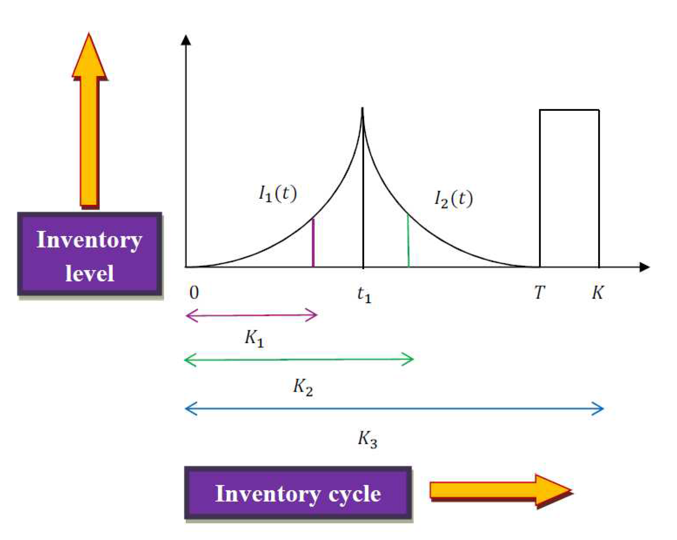
Figure 3.
Comparison of the average profit function for this model and Sana and Chaudhuri [48] model.
Figure 3.
Comparison of the average profit function for this model and Sana and Chaudhuri [48] model.
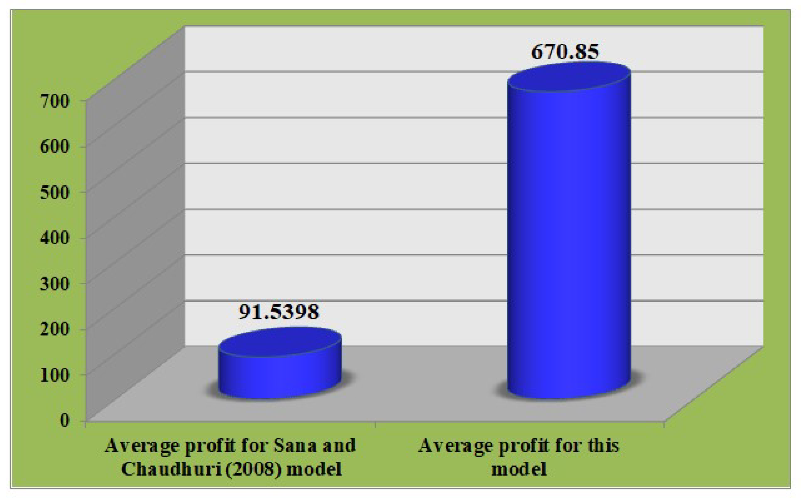
Figure 4.
Average profit versus inventory cycle’s duration (T) and selling price (P).
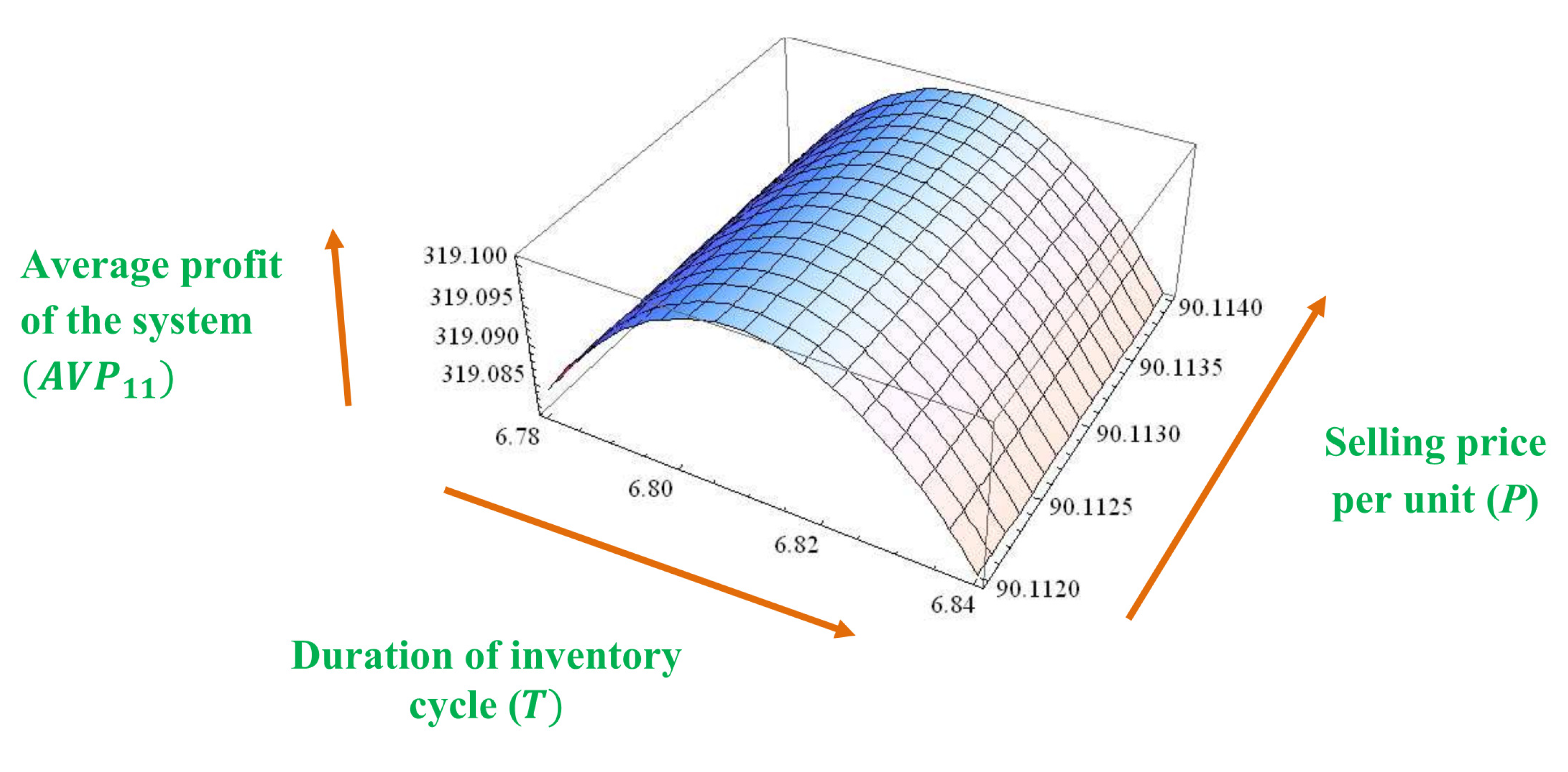
Figure 5.
Average profit versus inventory cycle’s duration (T) and selling-price (P).
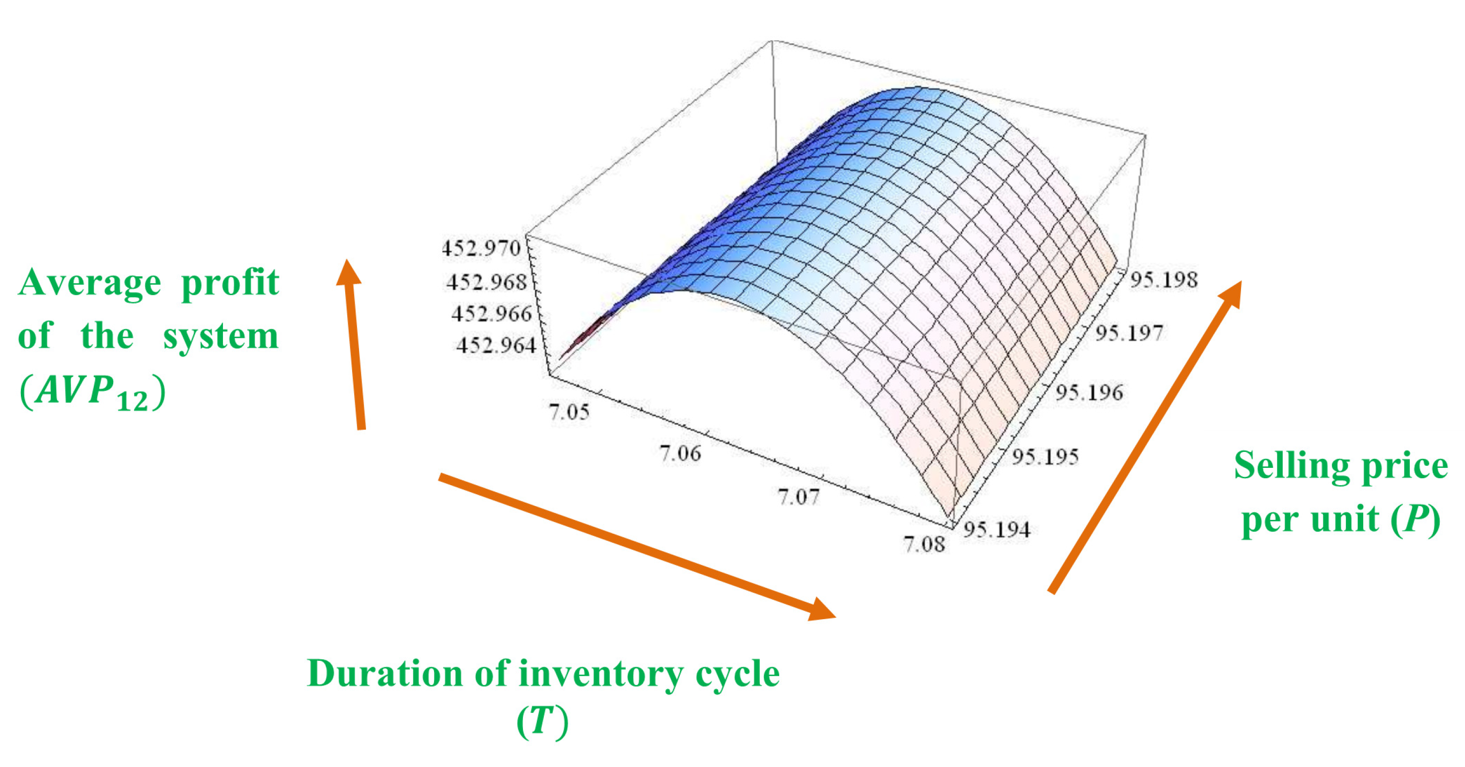
Figure 6.
Average profit versus inventory cycle’s duration (T) and selling-price (P).
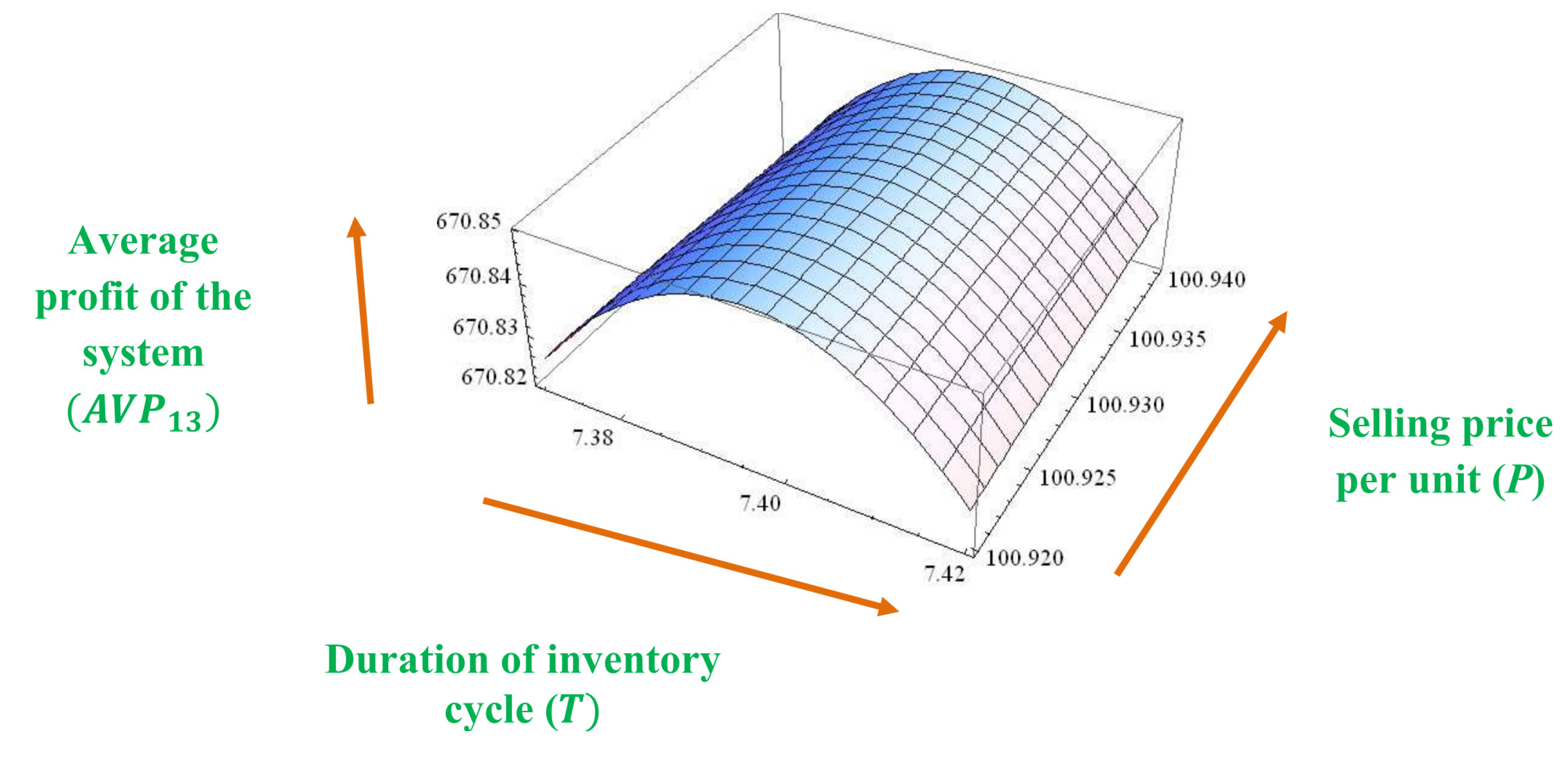
Figure 7.
Average profit against selling-price (P) and inventory cycle’s duration (T).

Figure 8.
Average profit versus inventory cycle’s duration (T) and selling-price (P).

Figure 9.
Average profit versus inventory cycle’s duration (T) and selling-price (P).
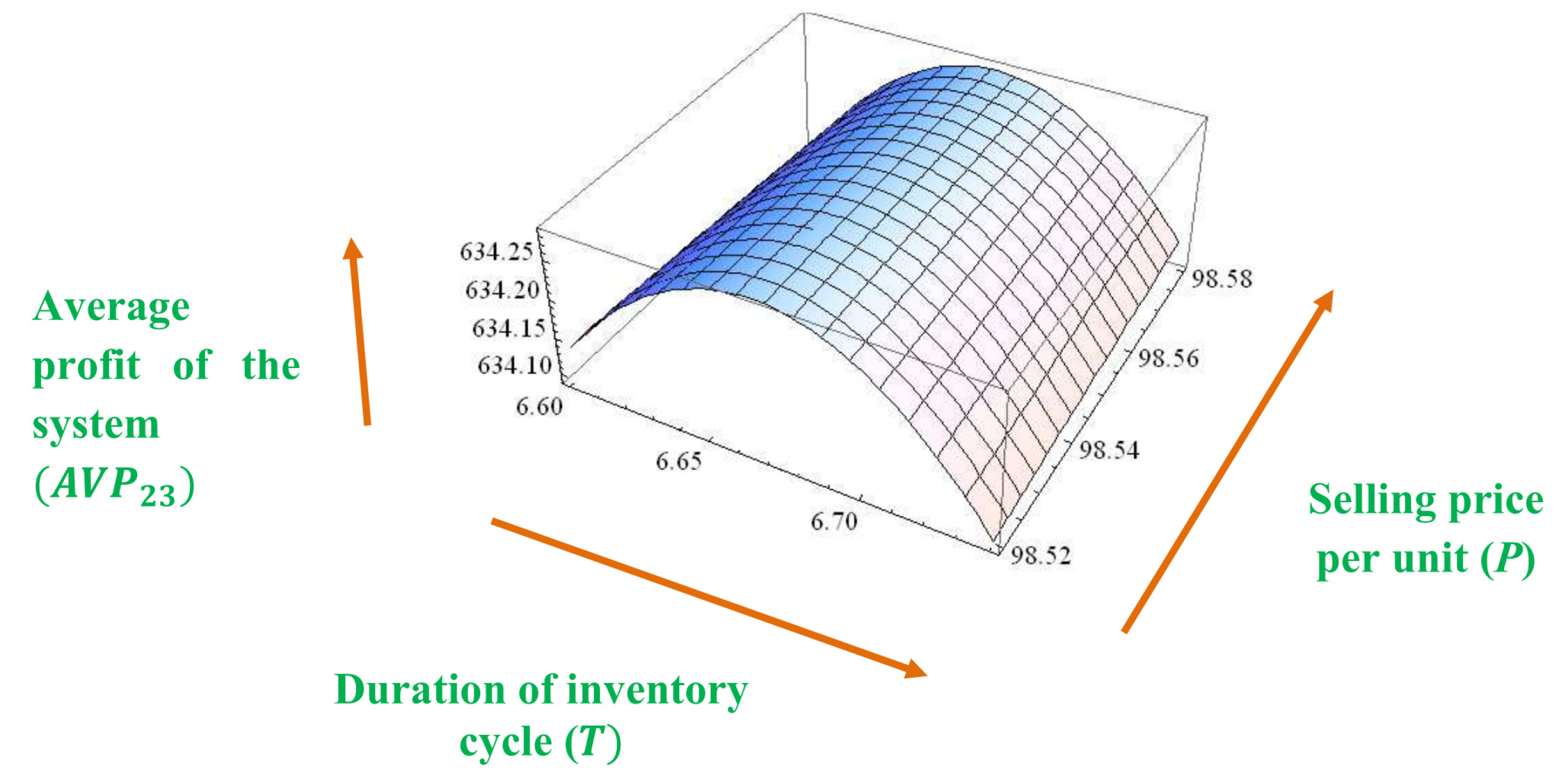
Figure 10.
Impact of variations for changes of distinct parameters on system’s average profit .

Figure 11.
Impact of variations for changes of distinct parameters on system’s average profit
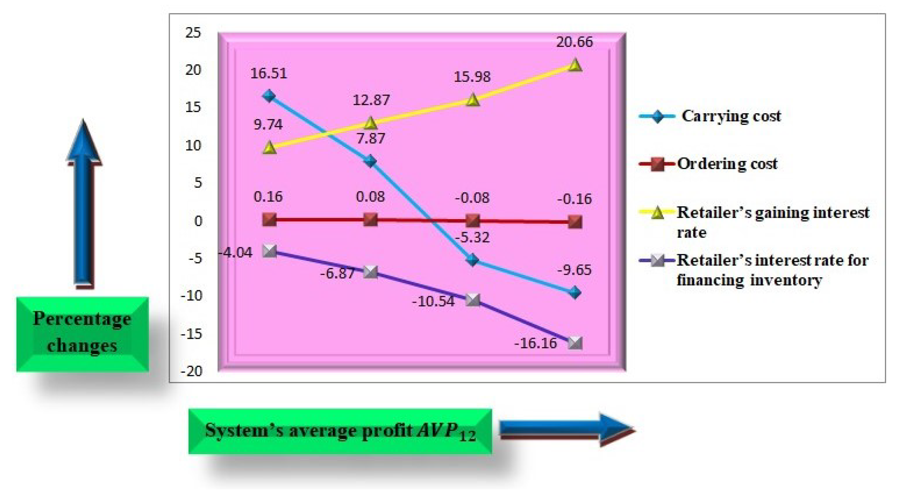
Figure 12.
Impact of variations for changes of distinct parameters on system’s average profit .
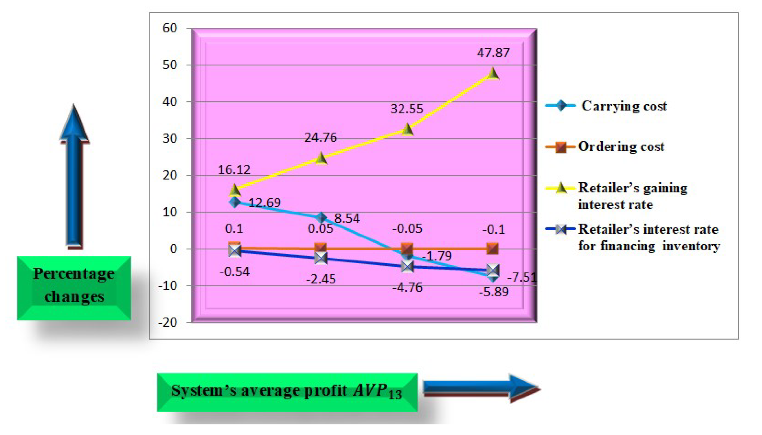
Figure 13.
Impact of variations for changes of distinct parameters on system’s average profit .

Figure 14.
Impact of variations for changes of distinct parameters on system’s average profit .
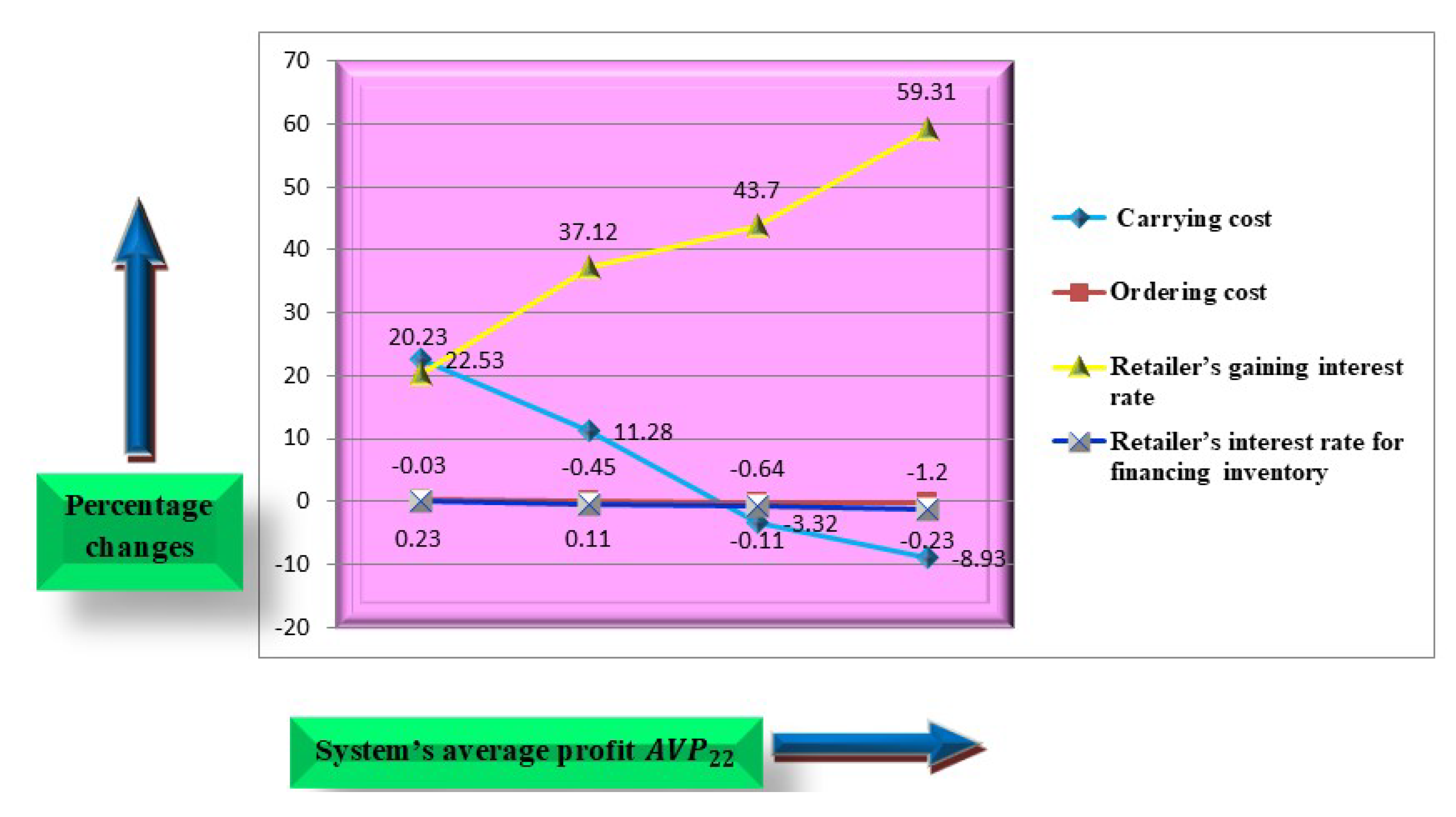
Figure 15.
Impact of variations for changes of distinct parameters on system’s average profit .
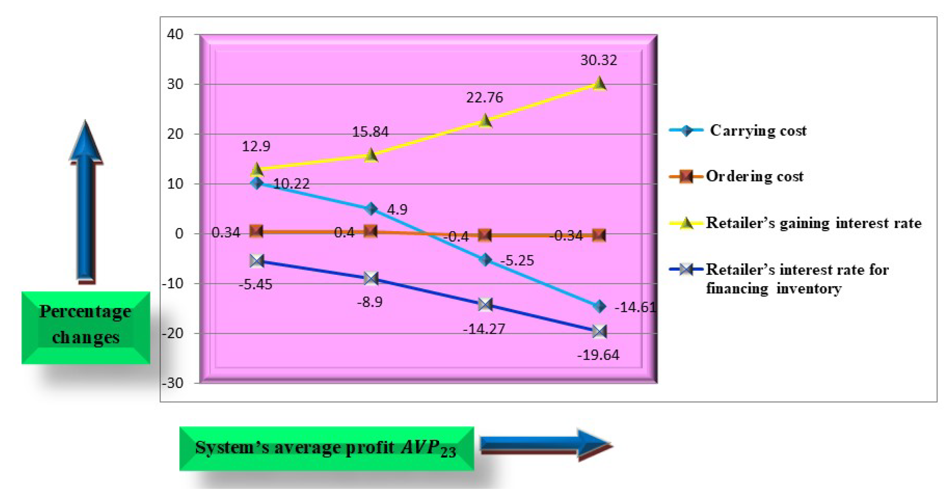
Figure 16.
Average profit versus inventory cycle’s duration (T) and selling-price (P).
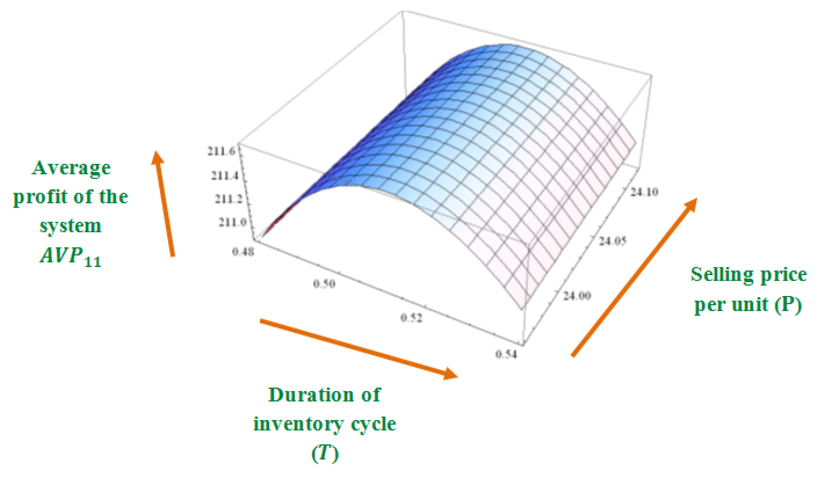
Figure 17.
Average profit versus inventory cycle’s duration (T) and selling-price (P).

Figure 18.
Average profit versus inventory cycle’s duration (T) and selling-price (P).
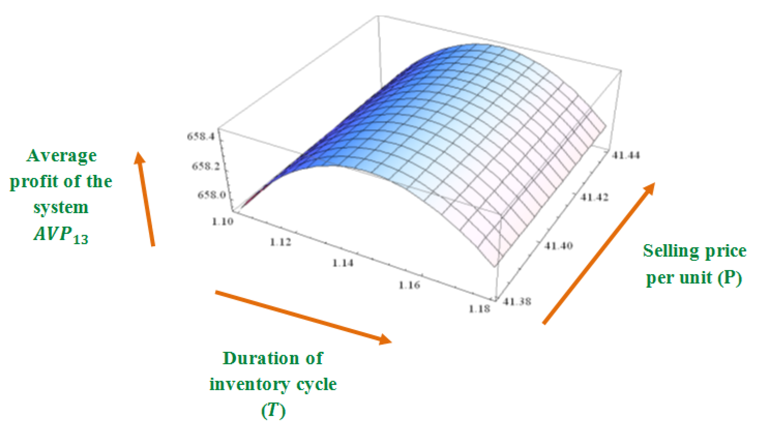
Figure 19.
Average profit versus inventory cycle’s duration (T) and selling-price (P).

Figure 20.
Average profit versus inventory cycle’s duration (T) and selling-price (P).
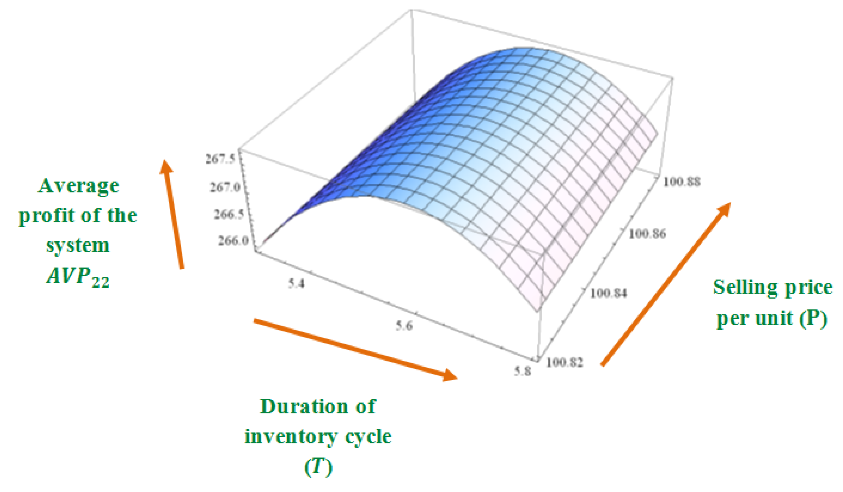
Figure 21.
Average profit versus inventory cycle’s duration (T) and selling-price (P).


Table 1.
Contribution Table of distinct Author(s).
| Author(s) | Demand (Price and Time Related) | Discount Policy | Trade-Credit Policy | Deterioration |
|---|---|---|---|---|
| Dey et al. [10] | Price related | - | - | - |
| Alfares and Ghaithan [14] | Price related | Quantity discount | - | - |
| Li et al. [19] | - | - | One level | - |
| Avinadav et al. [32] | Price and time related | - | - | Constant |
| Xu et al. [37] | - | Discount in price | - | - |
| Jaggi et al. [40] | - | - | Two level | - |
| Sarkar et al. [44] | Time related | - | - | - |
| Sarkar and Sarkar [45] | - | - | - | Variable |
| Teng and Chang [46] | Price related | - | - | Constant |
| Wu et al. [47] | - | - | - | Variable |
| This model | Price and time related | Discount in price | One level | Constant |
“-” means this concept does not exist in that study.
Table 2.
Sensitivity Analysis for distinct parameters.
| Parameters | Changes (in %) | ||||||
|---|---|---|---|---|---|---|---|
| −50% | 20.4 | 16.51 | 12.69 | 25.2 | 22.53 | 10.22 | |
| −25% | 10.28 | 7.87 | 8.54 | 12.53 | 11.28 | 4.9 | |
| +25% | −2.54 | −5.32 | −1.79 | −4.1 | −3.32 | −5.25 | |
| +50% | −7.76 | −9.65 | −7.51 | −11.74 | −8.93 | −14.61 | |
| −50% | 0.23 | 0.16 | 0.1 | 0.56 | 0.23 | 0.34 | |
| −25% | 0.11 | 0.08 | 0.05 | 0.28 | 0.11 | 0.4 | |
| +25% | −0.11 | −0.08 | −0.05 | −0.28 | −0.11 | −0.4 | |
| +50% | −0.23 | −0.16 | −0.1 | −0.56 | −0.23 | −0.34 | |
| −50% | 3.17 | 9.74 | 16.12 | 24.57 | 20.23 | 12.9 | |
| −25% | 4.53 | 12.87 | 24.76 | 30.77 | 37.12 | 15.84 | |
| +25% | 7.21 | 15.98 | 32.55 | 45.21 | 43.7 | 22.76 | |
| +50% | 9.56 | 20.66 | 47.87 | 58.1 | 59.31 | 30.32 | |
| −50% | −14.19 | −4.04 | −0.54 | −0.41 | −0.03 | −5.45 | |
| −25% | −20.3 | −6.87 | −2.45 | −1.43 | −0.45 | −8.9 | |
| +25% | −25.7 | −10.54 | −4.76 | −3.48 | −0.64 | −14.27 | |
| +50% | −31.45 | −16.16 | −5.89 | −5.71 | −1.2 | −19.64 |
© 2020 by the authors. Licensee MDPI, Basel, Switzerland. This article is an open access article distributed under the terms and conditions of the Creative Commons Attribution (CC BY) license (http://creativecommons.org/licenses/by/4.0/).
Share and Cite
MDPI and ACS Style
Saren, S.; Sarkar, B.; Bachar, R.K. Application of Various Price-Discount Policy for Deteriorated Products and Delay-in-Payments in an Advanced Inventory Model. Inventions 2020, 5, 50. https://doi.org/10.3390/inventions5030050
AMA Style
Saren S, Sarkar B, Bachar RK. Application of Various Price-Discount Policy for Deteriorated Products and Delay-in-Payments in an Advanced Inventory Model. Inventions. 2020; 5(3):50. https://doi.org/10.3390/inventions5030050
Chicago/Turabian StyleSaren, Sharmila, Biswajit Sarkar, and Raj Kumar Bachar. 2020. "Application of Various Price-Discount Policy for Deteriorated Products and Delay-in-Payments in an Advanced Inventory Model" Inventions 5, no. 3: 50. https://doi.org/10.3390/inventions5030050