
Efficient Model for Accurate Assessment of Frequency Support by Large Populations of Plug-in Electric Vehicles


Department of Electrical and Computer Engineering, Technical University of Crete, GR-73100 Chania, Greece
*
Author to whom correspondence should be addressed.
Inventions 2021, 6(4), 89; https://doi.org/10.3390/inventions6040089
Submission received: 30 October 2021
/
Revised: 13 November 2021
/
Accepted: 15 November 2021
/
Published: 18 November 2021
(This article belongs to the Collection Feature Innovation Papers)
Abstract
:In recent years, plug-in electric vehicles (PEVs) have gained immense popularity and are on a trajectory of constant growth. As a result, power systems are confronted with new issues and challenges, threatening their safety and reliability. PEVs are currently treated as simple loads due to their low penetration. However, as their numbers are growing, PEVs could potentially be exploited as distributed energy storage devices providing ancillary services to the network. Batteries used in PEVs are developed to deliver instantaneously active power, making them an excellent solution for system frequency support. This paper proposes a detailed dynamic model that is able to simulate frequency support capability from a large number of PEVs, using an innovative aggregate battery model that takes into account the most significant constraints at PEV and aggregate battery levels. The cost optimization algorithm, which is the most time-consuming process of the problem, is executed only at the aggregate battery level, thereby reducing the computational requirements of the model without compromising the obtained accuracy. The proposed method is applied to the power system of Crete exploiting detailed statistical data of EV mobility. It is proven that PEVs can effectively support power system frequency fluctuations without any significant deviation from their optimal operation.
1. Introduction
Fossil fuels are the most common source of energy in everyday life. In the US only, petroleum products accounted for 90% of the total energy used for transportation in 2020 [1]. In order to reduce the environmental footprint of the transportation sector, sustainable alternatives to internal combustion engines (ICEs), such as hydrogen- and electricity-driven engines, should be exploited. While hydrogen vehicles are still facing some issues according to safety, low efficiency, and limited capacity [2], plug-in electric vehicles (PEVs) have attracted a significant research interest. At the same time, the fast-growing penetration of PEVs in the global automobile market is now evident. In 2020, the electric vehicle fleet exceeded 10 million units globally, which is 41% higher than in 2019. Furthermore, international campaign EV30@30 launched by the Clean Energy Ministerial [3] pledges to achieve 30% market share for PEVs by 2030 to reach 250 million sales. Hence, a quite larger integration of PEVs is anticipated in the following years.
Even though PEVs are treated as typical loads for the time being, that can be fully altered if smart control and charging techniques are adopted. PEVs can be characterized by large flexibility that renders them ideal providers of ancillary services to the grid, such as frequency and voltage support [4]. Frequency support becomes extremely critical in future power systems due to the increasing penetration of renewable energy sources that amplify power system frequency instability. In this case, even small-frequency fluctuations can trigger large disturbances at the power system level. Vehicle-to-grid (V2G) technology [5,6] will further enhance the frequency support capacity of the grid. V2G operation is completely realistic, considering that an electric vehicle is parked for 90–95% of the time on an average day [7]. In this way, large populations of PEVs will be able to operate as controllable large powerplants or loads. V2G can be exploited for load frequency control (LFC) more effectively than conventional lumped battery energy storage systems (BESS) due to the significantly higher aggregated capacity and the high dispersion across the system [8]. In [9,10], it was shown that PEVs can stabilize load and frequency imbalances due to the fast response of their batteries, which are designed to withstand large and frequent power fluctuations [11].
In recent years a significant amount of research has been conducted on potential uses of PEVs. For instance, the work done in [12,13] proposed a control method for frequency regulation, considering also the expected state of charge (SOC) during PEV charging demands. In order to achieve load–frequency control, a large number of connected PEVs is needed. Thus, the concept of an aggregator [14,15,16] was introduced. The aggregated model represents the energy and power constraints of the entire PEV fleet [17], which acts as a virtual powerplant, providing frequency support to the grid [18,19]. Furthermore, the work done in [20] proposed a method for primary frequency control (PFC) using a simple constant droop characteristic, implemented in an isolated network model with a conventional generator and inertial emulation. Some other studies [21,22] suggested a better approach for frequency control, using fuzzy logic. The fuzzy controller receives information from PEV batteries and the grid, such as SOC and frequency deviation, controlling the output power in a more efficient and effective fashion.
The goal of this paper is to provide an accurate aggregate dynamic model capable of simulating frequency support capability by a large number of PEVs under various operating conditions, considering several PEV and system constraints. The suggested aggregation approach creates an equivalent battery model that contains detailed information about the battery characteristics and operational limitations for each vehicle. Afterward, methods for primary and secondary frequency support at the aggregator level are proposed. Instead of a simple frequency–load droop characteristic, fuzzy logic is implemented to develop a more efficient control approach that takes into account energy storage reserves. The accuracy of the proposed aggregation method is proven, while the proposed method for the simulation of the frequency support capacity of large PEV populations is applied to the island power system of Crete.
The remainder of this paper is divided into the following sections: Section 2 describes the calculation process that defines the aggregate model of the battery; Section 3 explains how the suggested frequency support model is implemented using fuzzy logic; Section 4 defines the power system models that are used in the proposed methodology to achieve an accurate frequency support simulation; Section 5 presents and discusses the simulation results; Finally, the conclusions drawn from our work are discussed in Section 6.
2. Formulation of the Aggregate Battery Model
Each modeled PEV has its own specifications in terms of battery capacity range and maximum charging–discharging rate. Furthermore, the departure time and the desired are determined using probability density functions obtained from real-world data. It is considered that every charging point is able to provide bidirectional flow of active power (load convention is used next). The stored energy in the battery of a PEV is estimated using the following equation:
where is the battery state of charge at time of the PEV connected to the -th charger, is the power the -th charging point exchanges with the network (when is positive, the PEV is charging), and is the charging/discharging efficiency coefficient of the PEV charging system.
Figure 1 represents the SOC trajectory the PEV follows between its connection time and disconnection time . and are the permissible minimum and maximum values of the PEV’s battery SOC. The initial state of charge at connection time is denoted with , and the desired state of charge at the disconnection time is denoted with . A maximum acceptable deviation of around is considered in this study. The red lines (, ) represent the dynamic lower and upper limits of the PEV’s SOC. In general, each SOC limit is defined by four points. More specifically, the points (, ), (, ), (, ), and (, ) define , while the points (, ), (, ), and (, ) define . Furthermore, , , , and , denote the timepoints where and increase or decrease with a constant rate of and , respectively.
In special cases where and/or , and can never reach the marginal values ( and ). The yellow line represents the optimal SOC trajectory during the PEV dwelling time according to the respective variation in electricity price. In a large electric power system hosting a large number of PEVs, calculating the optimal SOC trajectory for each individual PEV is clearly impractical and inefficient and leads to suboptimal and usually infeasible solutions for the electric power system. The quantities depicted in Figure 1 can be used to calculate a dynamic model of an aggregate equivalent battery representing a fleet of PEVs, as shown in Equations (8)–(13). Note that the total number of connected vehicles () is different for every minute () as electric vehicles are connected or disconnected from the network continuously.
Afterward, the optimum SOC trajectory of the equivalent battery representing the PEV population can be easily calculated. In this way, the optimal operation of large PEV populations can be achieved in a significantly short simulation time. In this approach, it is assumed that the PEVs are operated by large aggregators, which will be the case in the near future.
The objective function that needs to be minimized in order to calculate the optimal total power of the PEVs is
subject to the following:
- (1)
- Minimum and maximum power constraints,
- (2)
- Minimum and maximum SOC constraints,
- (3)
- Desired SOC at the end of the day,
The aggregated SOC satisfies the following equation:
where is the optimal aggregated power of the PEVs, is the forecasted electricity price, is the used time interval, and is the change in due to the continuous connection and disconnection of EVs, which is calculated as follows:
3. Frequency Support Implementation
The droop control method is utilized as an initial approach to support system frequency. Δf represents the frequency deviation from the nominal value (50 Hz). As shown in Figure 2, when is inside the dead-band (, ), no power is applied to support the frequency. The dead-band is added because the PEVs should not respond to minor frequency fluctuations, thus reducing the stress on their batteries. A typical dead-band width is 0.06% or 0.03 Hz [23]. The previous method is commonly used for frequency support in AC power systems. Since the mathematical models of power systems are usually nonlinear and more factors than frequency deviation should be considered, there is a need for more sophisticated algorithms. Hence, in this work, a fuzzy logic-based method was developed to estimate the appropriate power deviation, , that is needed to support the frequency. Fuzzy logic is a very powerful, nonlinear, and easy-to-use tool that leads to a more robust control than the conventional droop control method. The fuzzy controller proposed next was selected as it can provide a smooth and efficient frequency response taking into consideration several parameters and constraints of the examined system, while it is very easy to be implemented. Fuzzy logic-based controllers are very robust to forecast errors in contrast to several types of optimal control systems that are highly dependent on them. Moreover, with suitable parameter adjustment, in real time if needed, they can provide a nearly optimal response while maintaining the advantages mentioned before.
The first step of the process is the fuzzification stage, where inputs and outputs are fuzzified into membership functions as shown in Figure 3. Each fuzzy set corresponds to the linguistic variables such as very small (VS), small (S), average (A), big (B), and very big (VB) for the distance of the current SOC, , from its limits, frequency deviation , and power change deviation factor . Several tests indicated that the use of more linguistic variables does not affect the performance of the fuzzy controller. All three variables are normalized in the range of [0,1]. The value of is used to calculate the appropriate PEV power change depending on the frequency deviation as follows:
Fuzzy rules are executed using these linguistic variables to compute the fuzzy output, as shown in Table 1. During the defuzzification process, the output membership function of the fuzzy variable is mapped into a crisp value using a method based on centroids [24,25].
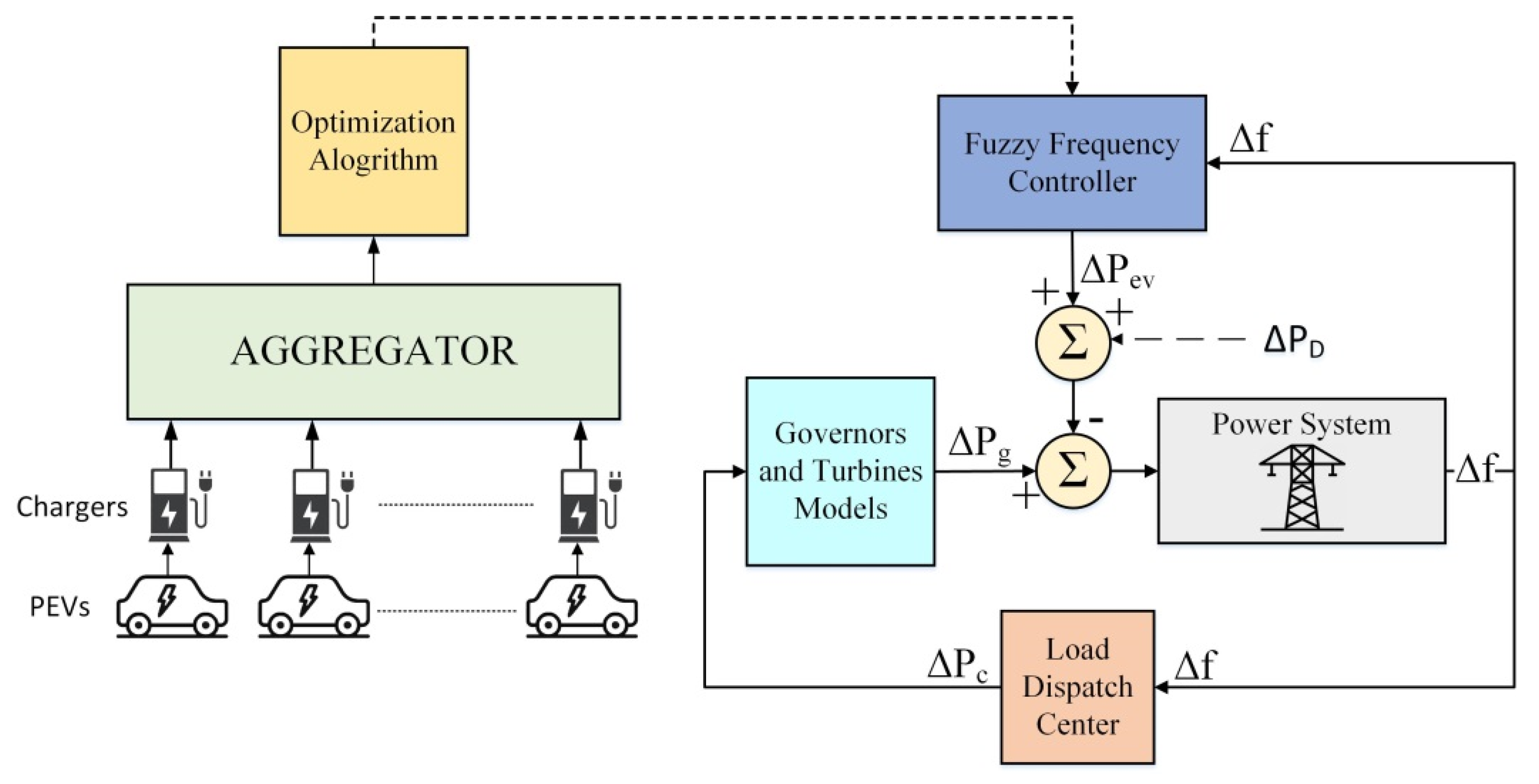
The fuzzy frequency controller used by the PEV aggregator works supportively with the existing frequency controller of the power system as shown in Figure 4. When a power disturbance occurs (), frequency deviates from its nominal value. The two frequency control systems detect the frequency deviation and try to deviate the power in the systems they control to exchange with the power grid in a manner that eliminates the resulting frequency deviation. For instance, when the load on the system is suddenly increased, the frequency drops. At that time, the applied fuzzy controller tries to reduce the PEV load or even inject some power into the grid if it is required. However, frequency deviation is not the only factor that determines how much power the PEV aggregator should exchange with the grid. The second fuzzy input, as shown in Figure 5, is called and represents the distance of the current aggregated SOC. For instance, if the PEV total power is positive, total SOC increases and approaches the limit while it deviates away from limit. In this case, represents the difference between the current SOC and . As SOC approaches its maximum value, gets closer to zero, and the capability of the PEV aggregator to support frequency during a negative frequency deviation is reduced. Therefore, the fuzzy controller should optimally ensure a tradeoff between the frequency deviation and the stored energy in the controlled fleet of PEV. A graphical representation of the output of the fuzzy controller with respect to the used decision variables is shown in Figure 6.
4. Description of Power System Model
Steam turbine driven power stations: Typical governor and steam turbine transfer functions are given below [26].
The transfer function used for the steam reheat stage is
where is the steam turbine governor time constant, is the steam turbine time constant, is the coefficient of reheat, and is the reheat time constant.
Hydroelectric power stations: The IEEEG2 model is usually used for power system LFC studies. It comprises the following transfer functions of the hydro speed governor and turbine [27,28]:
where, represents the water launching time or the water time constant, is the main servo time constant, is the speed governor rest time. and is the transient droop time constant.
Diesel engine driven power stations: The mathematical model of a diesel engine [29,30] consists of the mechanical speed-governing system Equation (26) and the diesel turbine dynamics Equation (27). It comprises the respective transfer functions.
where are the equivalent time constants of the speed governor, is the time constant of diesel power generation, and is the diesel turbine governor gain.
Gas turbine driven power stations: The simplified model of a typical gas turbine consists of four modules: the speed governing system, the valve positioner, the fuel system along with the combustor, and the turbine dynamics module. Normally gas turbines have three control circuits: speed control, temperature control, and acceleration control. Assuming that the temperature inside the combustion chamber will never be too high to damage the blades and there is no need for the acceleration controller to start or to shut down the turbine, the model can be simplified by using only the speed controller [31]. The respective transfer functions of the gas turbine unit are given in Equations (28)–(31).
where is the speed governor lead time constant, is the speed governor lag time constant, ,, are valve positioner time constants, is the combustion reaction time delay, is the fuel time constant, and is the compressor discharge time constant.
The control gains and time constants are suitably set for every type of generator in order simulate the response time and the amount of power generated for each one. Diesel and gas turbines have fast response time but less power generation due to high operating costs. Hydro and steam turbines are cheaper; thus, they take over most of the load over time due to the slower response time.
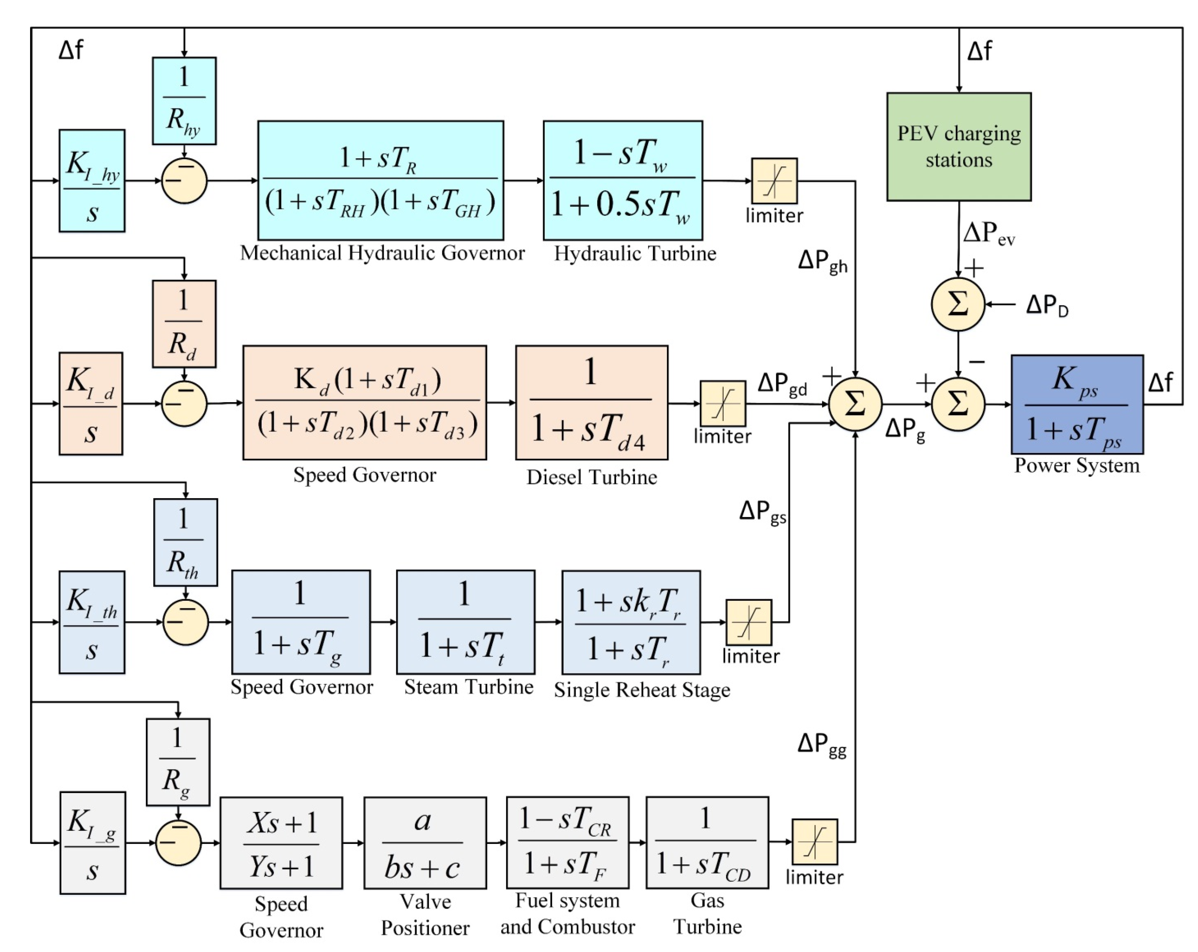
The models of the power generation units described above are interconnected as shown in Figure 7 [32]. In order to form the complete frequency control system of the electric power system, in this model, the response from the PEVs is included while the motion dynamics of the electric power generation system are modeled as a first-order transfer function with gain and time constant .
5. Case Study
The proposed aggregation method is able to deal with a large number of chargers. Whenever a vehicle arrives, it is connected to an unoccupied charger for the desired amount of time. As previously stated, instead of optimizing the charging cost of each PEV battery separately, an equivalent battery representing the population of PEVs is developed. Thus, the simulation time required to obtain the optimal charging power trajectory is reduced drastically as the most time-consuming process of the charging cost optimization is executed only once. We would like to note at this point that no optimization method can lead to the optimal solution with absolute certainty in large-scale problems, which also depend on the forecast of some inputs of the problem, e.g., the electricity price forecast. Moreover, in electric power system-scale applications, the cost is more effectively reduced at the aggregator level, while the electric power system constraints can be dealt more effectively only at this level.
In order to assess the accuracy of the proposed aggregation method, the SOC trajectory for each PEV is first optimized with regard to the resulting charging cost, the arrival and departure times, and battery constraints.
Five categories of PEVs were selected according to their price range. The battery specifications, as shown in Table 2, were estimated by calculating the mean values of 10 existing vehicle types of each category. Furthermore, regarding the arrival and departure times, real-life distributions were implemented, considering several activity types such as home, work, shop, and social [33,34].
Figure 8 depicts the obtained optimal SOC trajectories of the PEVs connected to one of the chargers.
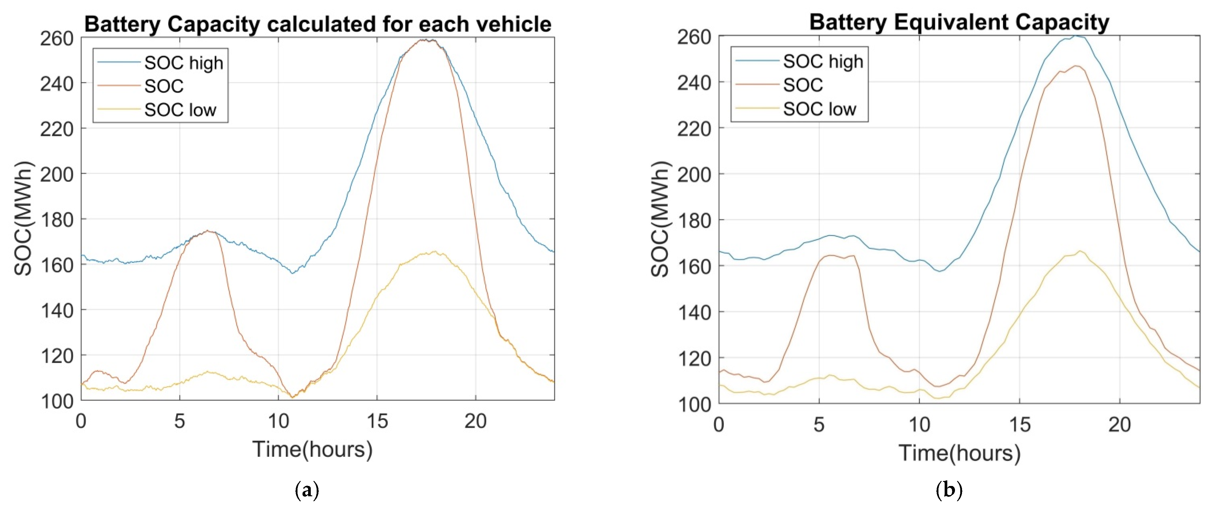
In Figure 9, the aggregated results of the optimal SOC trajectory of 20,000 PEVs using the two optimization approaches are shown, namely, optimization at PEV level and optimization at the equivalent aggregated battery level. The calculation time required by the first approach was 55 min, whereas it was only 4.3 min in the second approach. It becomes apparent from the obtained results that the optimal SOC trajectories obtained with the two approaches are almost identical.
In addition to the assessment of the accuracy of the equivalent battery model regarding its technical characteristics, frequency response was assessed. Figure 10 illustrates how the fuzzy controller responds to frequency changes when implemented independently on each battery, as well as when it is applied to the equivalent battery model. In this simulation, 1000 PEVs were utilized. In the case that a fuzzy frequency controller was applied to each car, the required simulation time was approximately 2185 s or 37 min. On the contrary, when the frequency controller was applied on the equivalent battery, simulation time was dramatically reduced to 2.17 s. As the frequency response obtained in both approaches is almost identical, the equivalent battery model is highly preferable due to the enormous reduction in the simulation time and the high accuracy it provides. The advantage of the simulation time reduction becomes even more substantial when hundreds of thousands, if not millions, of PEVs are connected to the electrical network.
The simulation is based on the power system of Crete which has a total installed power generation capacity of 820.02 MW with 27 power generators. Table 3 depicts the generation capacity of each generator. The figures below were calculated for August, where Crete’s power grid is at maximum strain, to assess how effectively PEVs contribute to frequency support. The total load for this operating point was 570 MW (gas turbines: 250 MW, steam turbines: 188 MW, diesel turbines: 132 MW).
The parameters of the power system model [35], as shown in Figure 7, are given in Table 4; 100 MVA base power and 50 Hz base frequency were used.
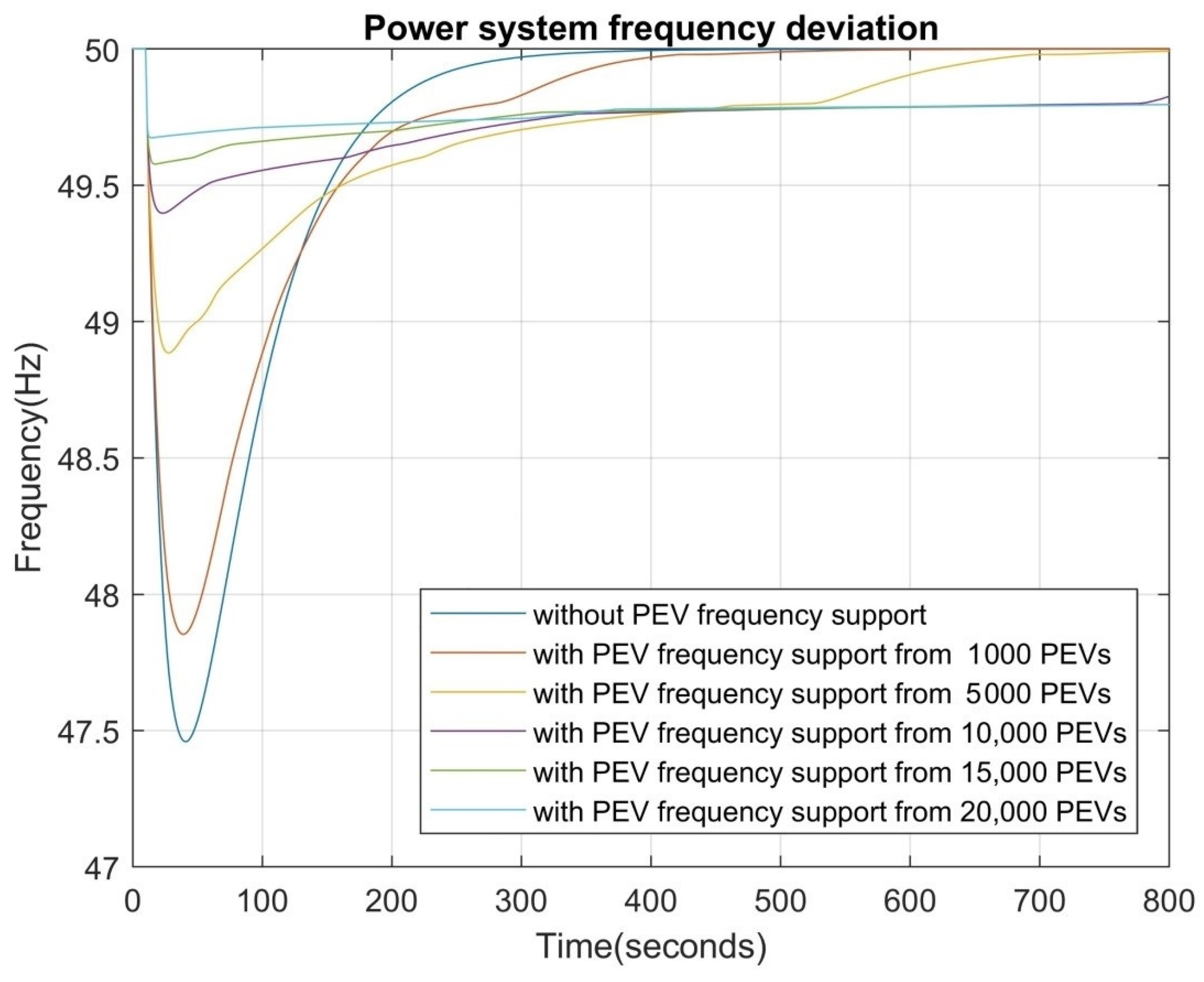
The effectiveness of frequency support provided by the PEV aggregator is highly dependent on the number of the PEVs. Assuming that 10% of all vehicles in Crete will be electric by 2030, a fleet of 50,000 PEVs will be available at that time. As shown in Figure 11, if there was no PEV frequency support, a 75 MW load step increase would cause a frequency drop under 47.5 Hz, resulting in a highly possible desynchronization of the system. On the contrary, using the PEV frequency support capability, frequency can be supported efficiently, especially when a significant number of electric vehicles are connected to the grid. Moreover, Figure 12 shows the obtained change in the power the PEVs exchange with the network with regard to their number.
Depending on the magnitude of the load change, the same number of vehicles can apply a different change to their power demand. In Figure 13, the response of 5,000 PEVs is shown with respect to the system load change.
The total number of PEVs is not the only factor that determines the amount of additional power drawn or delivered to the grid. For example, when system load decreases, PEVs must absorb more power to support the frequency. However, if PEVs are already absorbing the maximum amount of power, it is impossible to support the frequency. The same issue occurs when system load increases and the PEVs are already providing to the grid their maximum power.
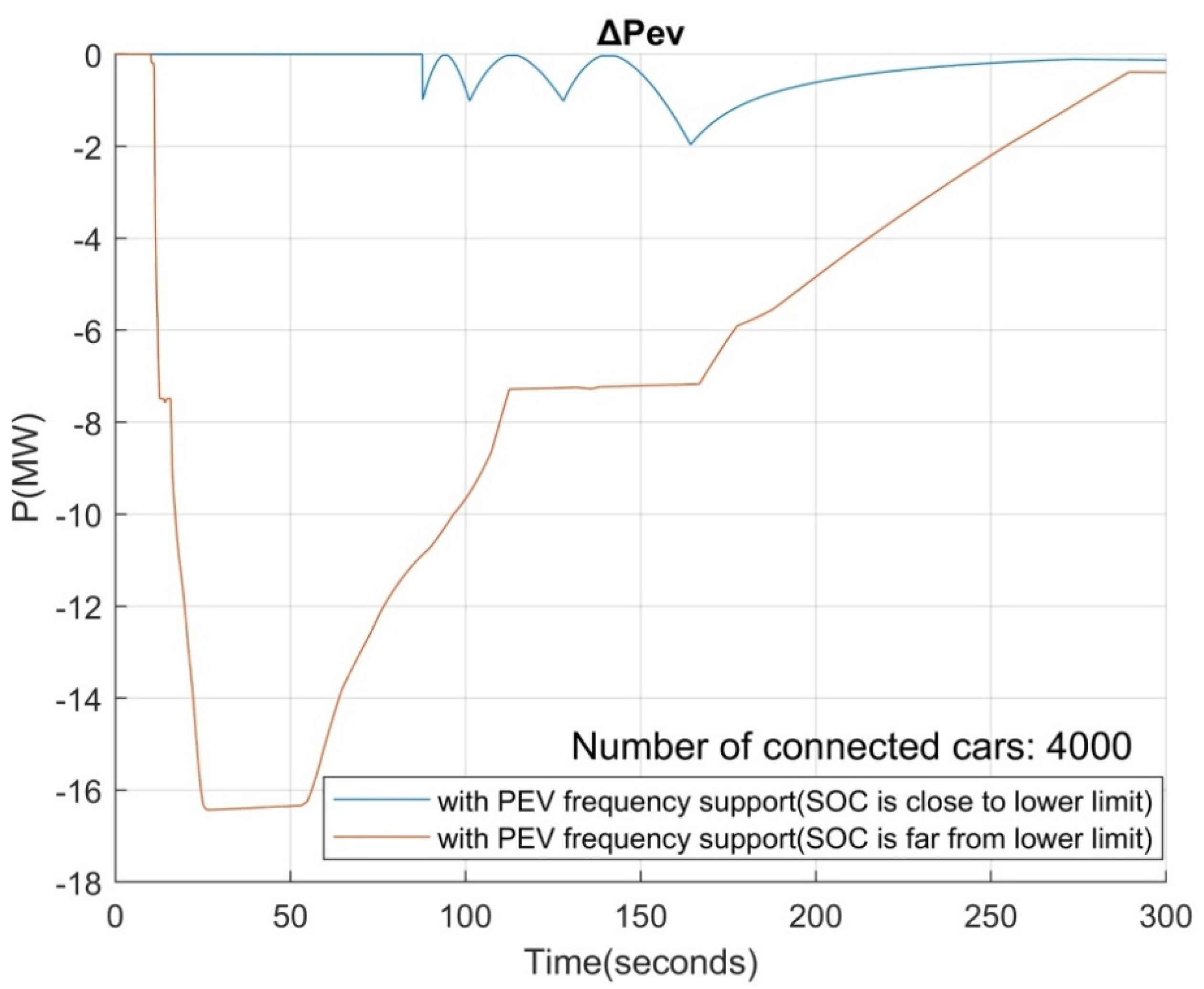
Another significant factor that affects the frequency support capability of the PEVs is the proximity of their aggregated current state of charge to the respective lower or upper limits. In order to justify this remark, two cases were simulated, as shown in Figure 14. Both of them employed the same number of PEV in order to ensure the same aggregated power capacity. The power grid was also subjected to the same increase of load. The only difference between the two cases was the proximity of the aggregated SOC to its lower limit. When system load increases, additional power will flow from the vehicles to the grid, lowering the SOC level of the equivalent battery. If SOC is already close to the lower limit, as shown in Figure 14, less or even no power will be injected to the grid. Similar behavior would be observed if system load was reduced and the SOC of the equivalent battery was closer to its upper limit.
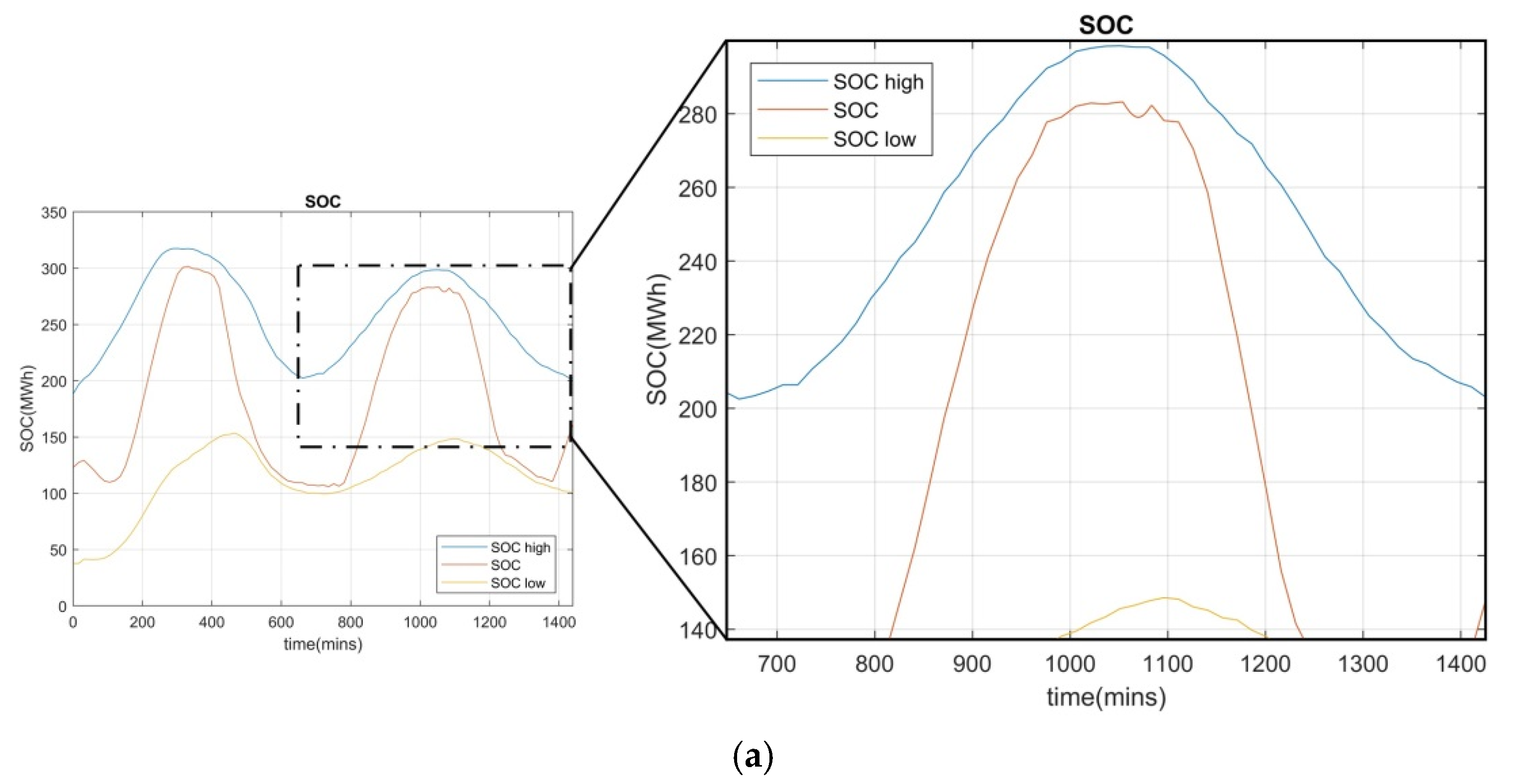
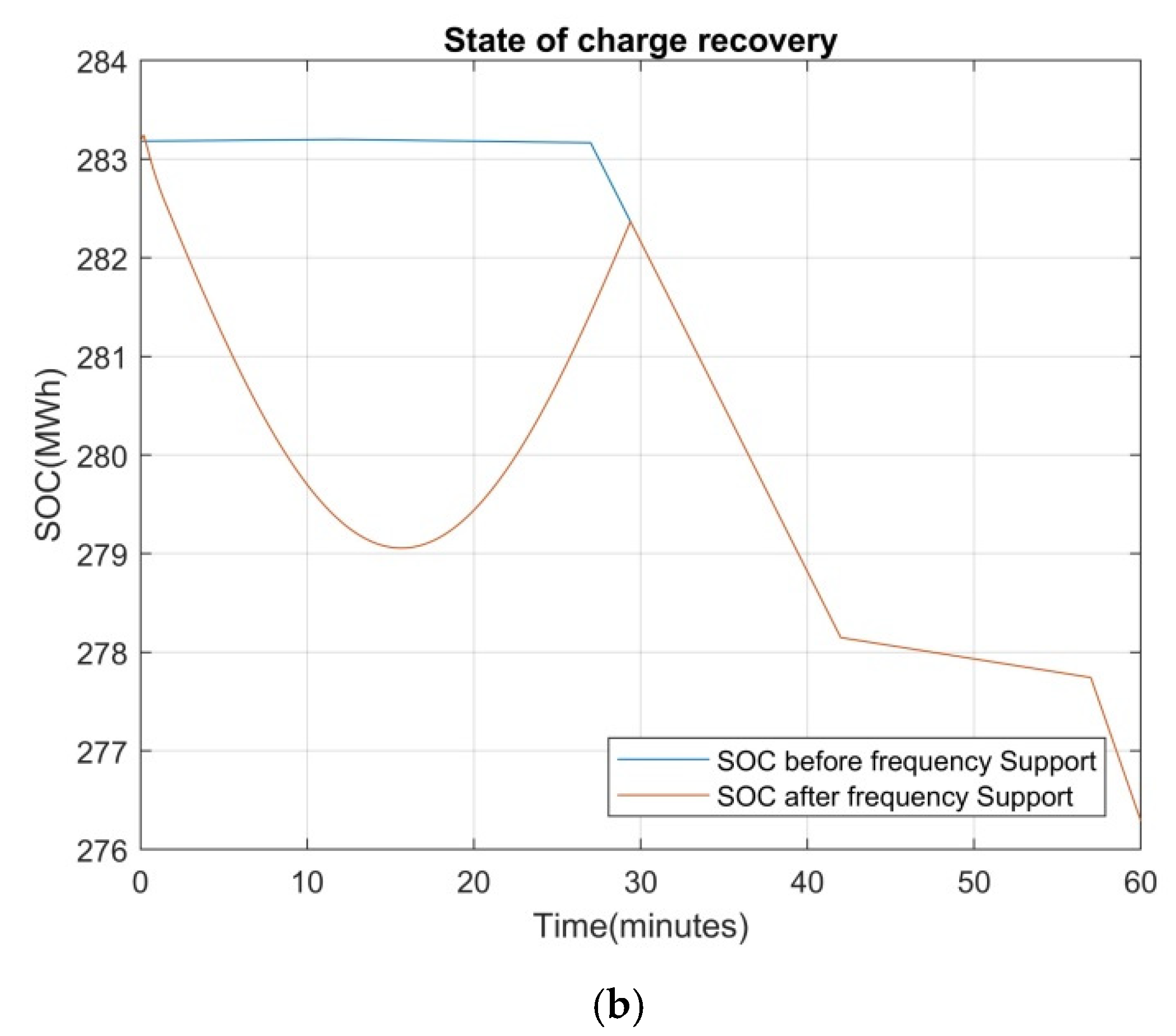
Another issue that occurs during frequency support by the PEVs is that the SOC of the equivalent battery will deviate from the optimal precalculated trajectory. To solve this, two approaches can be proposed. According to the first approach the optimal SOC can be recalculated when frequency support is no longer required. This means that the optimization algorithm for the calculation of the optimal SOC trajectory must be rerun for the remainder of the 24 h time period. This will add extra calculation time. The second option is to try reaching the precalculated SOC by appropriately increasing or decreasing the PEV power until the aggregated SOC coincides with the optimal precalculated one. As shown in Figure 15a, a frequency drop occurs at the 1060th minute of the examined 24 h time period. The PEVs provide additional power to the grid and the overall SOC drops. To reach the optimal trajectory, the power absorbed by the PEVs is gradually increased, and the SOC gradually returns to the optimal trajectory, as illustrated in Figure 15b. The blue line depicts the optimal SOC trajectory in the absence of frequency support, whereas the red line depicts the SOC trajectory after frequency support and during SOC restoration.
6. Discussion
In this paper, a method to obtain an efficient equivalent aggregate battery model for a large number of plug-in electric vehicles able to accurately assess frequency support services to the electrical grid was proposed. The model comprises detailed information on individual PEV batteries, such as stored energy capacity power limitations and real-world mobility data in order to model the dynamic behavior of the aggregate battery. The optimal SOC trajectory for each vehicle, as well as for the equivalent battery, is calculated using a classical optimization approach considering all battery technical constraints and arrival/departure times of the PEVs. Furthermore, a fuzzy logic-based frequency controller was developed in order to compute the appropriate amount of power that PEVs should exchange with the grid during frequency support mode of operation. The proposed method was evaluated on Crete’s electrical power system for several operation scenarios and PEV penetration. The respective simulations were conducted to demonstrate the superiority of the proposed technique in terms of computation time and accuracy. Lastly, the conducted simulations could be useful in deciding the number of PEVs required to successfully eliminate significant frequency disturbances without violating any battery restrictions for different power system operation scenarios. The suggested model can be highly beneficial for the transmission system operators in terms of system planning. Moreover, the model is fully parametric as it includes a large number of system parameters and technical characteristics, allowing its application to any power system. In future work, the technical problem of the real-time optimal power distribution at the PEV level can be examined.
Author Contributions
Conceptualization, F.D.K.; methodology, F.D.K.; software, M.D.; validation, F.D.K. and M.D.; formal analysis, F.D.K. and M.D.; investigation, F.D.K. and M.D.; resources, F.D.K.; data curation, F.D.K.; writing—original draft preparation, M.D.; writing—review and editing, F.D.K. and M.D.; visualization, F.D.K.; supervision, F.D.K.; project administration, F.D.K. All authors have read and agreed to the published version of the manuscript.
Funding
This research received no external funding.
Institutional Review Board Statement
Not applicable.
Informed Consent Statement
Not applicable.
Data Availability Statement
The probability functions for arrival and departure times were derived by processing a large set of real-world data provided by National Household Travel Survey (NHTS) available at: https://nhts.ornl.gov/2009/pub/stt.pdf (accessed on 13 September 2021).
Conflicts of Interest
The authors declare no conflict of interest.
Nomenclature
| The current time of simulation (min) | |
| The arrival time of the vehicle (min) | |
| The departure time of the vehicle (min) | |
| State of charge of PEV’s battery (kWh) | |
| Initial state of charge | |
| The maximum of PEV’s battery (kWh) | |
| The minimum of PEV’s battery (kWh) | |
| The desired at PEV’s departure time (kWh) | |
| The dynamic upper limit of PEV’s (kWh) | |
| The dynamic lower limit of PEV’s (kWh) | |
| The time that starts to converge to target or (min) | |
| The time that starts to converge to target or (min) | |
| The maximum power the PEV can exchange with the grid (kW) | |
| The minimum power the PEV can exchange with the grid (kW) | |
| The power that PEV exchanges with the grid (kW) | |
| Electricity price (EUR/kWh) | |
| Time step (min) | |
| The number of PEVs | |
| Total power change of PEVs during frequency support mode of operation (ΜW) | |
| Power demand change (ΜW) | |
| Generation power change during frequency support mode of operation (ΜW) |
References
- U.S. Energy Information Administration. Use of Energy Explained. Energy Used for Transportation. May 2019. Available online: https://www.eia.gov/energyexplained/use-of-energy/transportation.php (accessed on 10 November 2021).
- Mori, D.; Hirose, K. Recent challenges of hydrogen storage technologies for fuel cell vehicles. Int. J. Hydrogen Energy 2009, 34, 4569–4574. [Google Scholar] [CrossRef]
- Clean Energy Minestrial: EV30@30 Campaign. Available online: https://www.cleanenergyministerial.org/campaign-clean-energy-ministerial/ev3030-campaign (accessed on 10 November 2021).
- Galus, M.D.; Vaya, M.G.; Krause, T.; Andersson, G. The role of electric vehicles in smart grids. Wiley Interdiscip. Rev. Energy Environ. 2013, 2, 384–400. [Google Scholar] [CrossRef]
- Yilmaz, M.; Krein, P.T. Review of the impact of vehicle-to-grid technologies on distribution systems and utility interfaces. IEEE Trans. Power Electron. 2013, 28, 5673–5689. [Google Scholar] [CrossRef]
- Kalaitzakis, I.; Dakanalis, M.; Kanellos, F.D. Optimal Power Management for Residential PEV Chargers with Frequency Support Capability. In Proceedings of the 10th International Conference on Modern Circuits and Systems Technologies (MOCAST), Thessaloniki, Greece, 5–7 July 2021; pp. 1–4. [Google Scholar]
- Markel, A.J.; Bennion, K.; Kramer, W.; Bryan, J.; Giedd, J. Field Testing Plug-In Hybrid Electric Vehicles with Charge Control Technology in the Xcel Energy Territory; No. NREL-TP-550-46345; National Renewable Energy Laboratory: Golden, CO, USA, 2009.
- Energy Information Administration. Inventory of Electric Utility Power Plants in the United States 2000; DOE/EIA-0095 (2000), Table I; U.S. Department of Energy: Washington, DC, USA, 2002.
- Liu, H.; Hu, Z.; Song, Y.; Lin, J. Decentralized vehicle-to-grid control for primary frequency regulation considering charging demands. IEEE Trans. Power Syst. 2013, 28, 3480–3489. [Google Scholar] [CrossRef]
- Mu, Y.; Wu, J.; Ekanayake, J.; Jenkins, N.; Jia, H. Primary frequency response from electric vehicles in the Great Britain power system. IEEE Trans. Smart Grid 2013, 2, 1142–1150. [Google Scholar] [CrossRef]
- Kempton, W.; Tomic, J. Vehicle-to-grid power implementation: From stabilizing the grid to supporting large-scale renewable energy. J. Power Sources 2005, 1, 280–294. [Google Scholar] [CrossRef]
- Liu, H.; Qi, J.; Wang, J.; Li, P.; Wei, H. EV Dispatch Control for Supplementary Frequency Regulation Considering the Expectation of EV Owners. IEEE Trans. Smart Grid 2018, 4, 3763–3772. [Google Scholar] [CrossRef] [Green Version]
- Liu, H.; Hu, Z.; Song, Y.; Wang, J.; Xie, X. Vehicle to Grid Control for Supplementary Frequency Regulation Considering charging demands. IEEE Trans. Power Syst. 2015, 6, 3110–3119. [Google Scholar] [CrossRef]
- Konstantinidis, G.; Kanellos, F.D.; Kalaitzakis, K. A simple multi-parameter method for efficient charging scheduling of electric vehicles. Appl. Syst. Innov. 2021, 4, 58. [Google Scholar] [CrossRef]
- Escudero-Garzas, J.J.; Garcia-Armada, A.; Seco-Granados, G. Fair Design of Plug-in Electric Vehicles Aggregator for V2G Regulation. IEEE Trans. Veh. Technol. 2012, 61, 3406–3419. [Google Scholar] [CrossRef] [Green Version]
- Sung, D.K.; Ko, K.S. The Effect of EV Aggregators With Time-Varying Delays on the Stability of a Load Frequency Control System. IEEE Trans. Power Syst. 2018, 1, 669–680. [Google Scholar]
- Zhang, H.; Hu, Z.; Xu, Z.; Song, Y. Evaluation of Achievable Vehicle-to-Grid Capacity Using Aggregate PEV Model. IEEE Trans. Power Syst. 2017, 1, 784–794. [Google Scholar] [CrossRef]
- Han, S.; Han, S.; Sezaki, K. Development of an optimal vehicle-to grid aggregator for frequency regulation. IEEE Trans. Smart Grid 2010, 1, 65–72. [Google Scholar]
- Wang, M.; Mu, Y.; Shi, Q.; Jia, H.; Li, F. Electric Vehicle Aggregator Modeling and Control for Frequency Regulation Considering Progressive State Recovery. IEEE Trans. Smart Grid 2020, 5, 4176–4189. [Google Scholar] [CrossRef]
- Almeida, P.R.; Soares, F.; Lopes, J.P. Electric vehicles contribution for frequency control with inertial emulation. Electr. Power Syst. Res. 2015, 127, 141–150. [Google Scholar] [CrossRef] [Green Version]
- Datta, M. Fuzzy Logic Based Frequency Control by V2G Aggregators. In Proceedings of the IEEE 5th International Symposium on Power Electronics for Distributed Generation Systems, Galway, Ireland, 24–27 June 2014. [Google Scholar]
- Falahati, S.; Taher, S.A.; Shahidehpour, M. Grid frequency control with electric vehicles by using of an optimized fuzzy controller. Appl. Energy 2016, 178, 918–928. [Google Scholar] [CrossRef]
- Lee, K.A.; Yee, H.; Teo, C. Self-tuning algorithm for automatic generation control in an interconnected power system. Electr. Power Syst. Res. 1991, 2, 157–165. [Google Scholar] [CrossRef]
- Altas, I.H.; Neyens, J. A fuzzy logic decision maker and controller for reducing load frequency oscillations in multi-area power systems. In IEEE Power Engineering Society General Meeting; IEEE: Montreal, QC, Canada, 2006. [Google Scholar]
- Kanellos, F.D. Multiagent-System-Based Operation Scheduling of Large Ports’ Power Systems with Emissions Limitation. IEEE Syst. J. 2019, 2, 1831–1840. [Google Scholar] [CrossRef]
- Dulau, M.; Bica, D. Simulation of Speed Steam Turbine Control System. In Proceedings of the 7th International Conference Interdisciplinarity in Engineering, Tirgu Mures, Romania, 10–11 October 2013; pp. 716–722. [Google Scholar]
- Caballero, R.; Duhé, J.-F. Comparative Analysis for the Load Frequency Control Problem in Steam and Hydraulic Turbines using Integral Control, Pole Placement and Linear Quadratic Regulator. Global Partnerships for Development and Engineering Education. In Proceedings of the 15th LACCEI International Multi-Conference for Engineering, Education and Technology, Boca Raton, FL, USA, 19–21 July 2017. [Google Scholar]
- Surianu, F.D. Mathematical Modelling and Numerical. Simulation of the Dynamic Behavior of Thermal and Hydro Power Plants; INTECH Open Access Publisher: Timisoara, Romania, 2012. [Google Scholar]
- Karnavas, Y.L.; Papadopoulos, D.P. Power generation control of a wind-diesel system using fuzzy logic and pi-sigma networks. In Proceedings of the 12th International Conference on Intelligent Systems Application to Power Systems (ISAP ’03), Lemnos Island, Greece, 31 August–3 September 2003. [Google Scholar]
- Wagle, R.; Pariyar, B. Mathematical Modeling of Isolated Wind-Diesel-Solar Photo Voltaic Hybrid Power System for Load Frequency Control. Int. J. Sci. Res. 2018, 7, 960–966. [Google Scholar]
- Krpan, M.; Kuzle, I. The Mathematical Model of a Wind Power Plant and a Gas Power Plant. Master’s Thesis, University of Zagreb, Faculty of Electrical Engineering and Computing, Zagreb, Croatia, September 2016. [Google Scholar]
- Barisal, A.K. Comparative performance analysis of teaching learning-based optimization for automatic load frequency control of multi-source power systems. Int. J. Electr. Power Syst. Res. 2015, 66, 67–77. [Google Scholar] [CrossRef]
- Kanellos, F.D. Optimal Scheduling and Real-Time Operation of Distribution Networks With High Penetration of Plug-In Electric Vehicles. IEEE Syst. J. 2021, 15, 3938–3947. [Google Scholar] [CrossRef]
- Santos, A.; McGuckin, N.; Nakamoto, H.Y.; Gray, D.; Liss, S. Summary of Travel Trends: 2009 National Household Travel Survey. Available online: https://nhts.ornl.gov/2009/pub/stt.pdf (accessed on 13 September 2021).
- Ramakrishna, K.S.S.; Sharma, P.; Bhatti, T.S. Automatic generation control of interconnected power system with diverse sources of power generation. Int. J. Eng. Sci. Technol. 2010, 5, 51–65. [Google Scholar] [CrossRef]
Figure 1.
State-of-charge trajectory of an electric vehicle connected to a charger at time and disconnected at time .
Figure 1.
State-of-charge trajectory of an electric vehicle connected to a charger at time and disconnected at time .
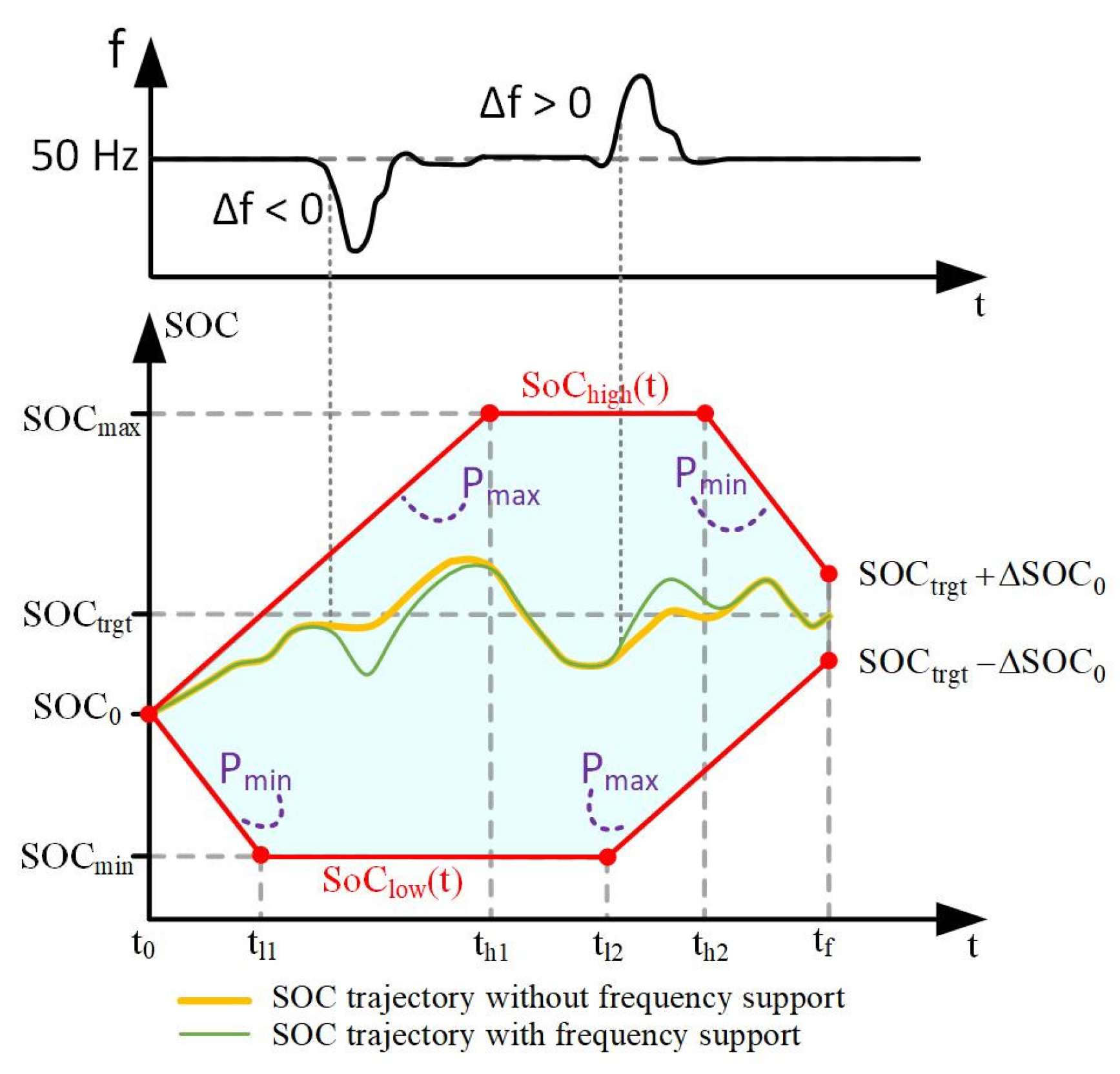
Figure 2.
Droop frequency control scheme.
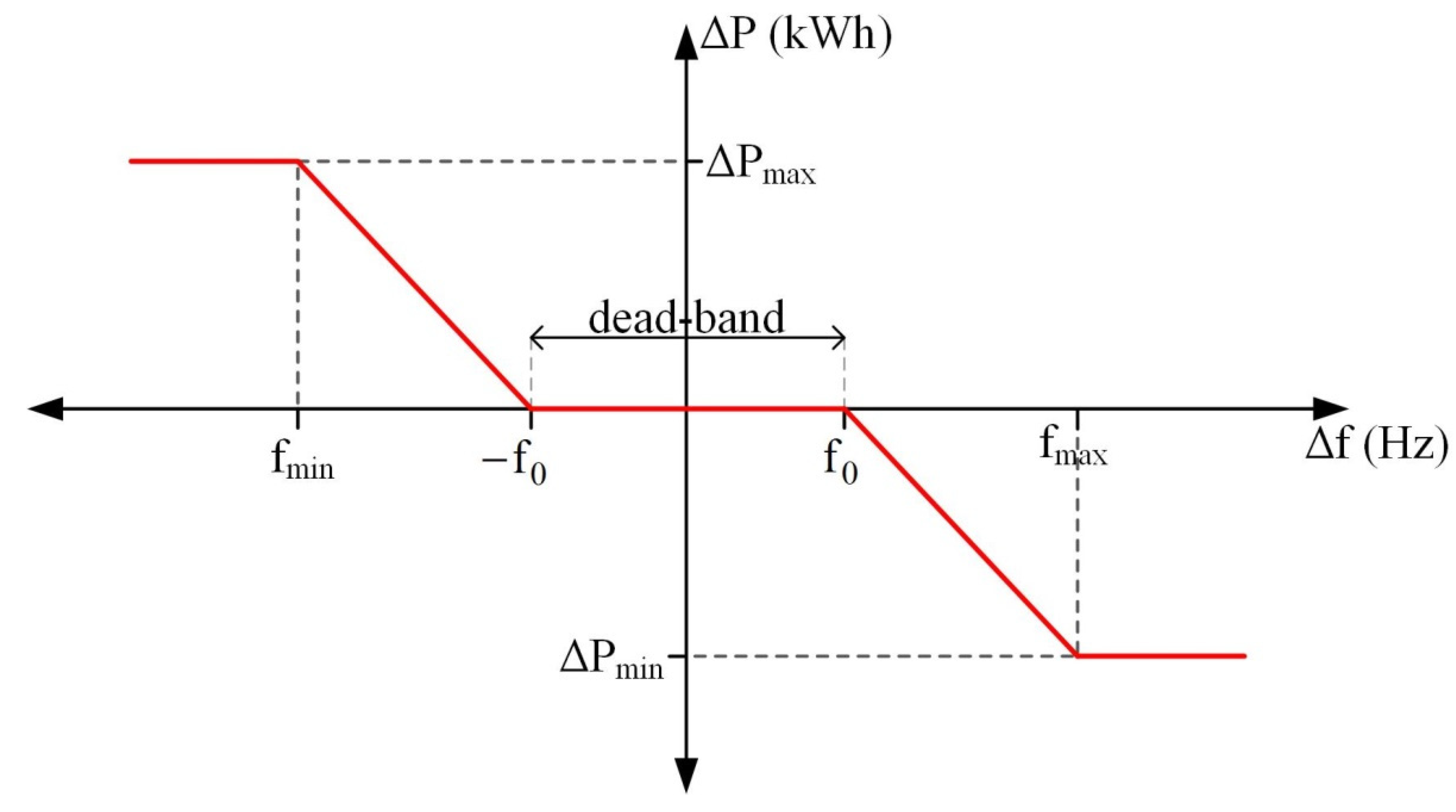
Figure 3.
Membership functions of the fuzzy variables: (a) ; (b) frequency deviation from 50 Hz; (c) power change coefficient .
Figure 3.
Membership functions of the fuzzy variables: (a) ; (b) frequency deviation from 50 Hz; (c) power change coefficient .
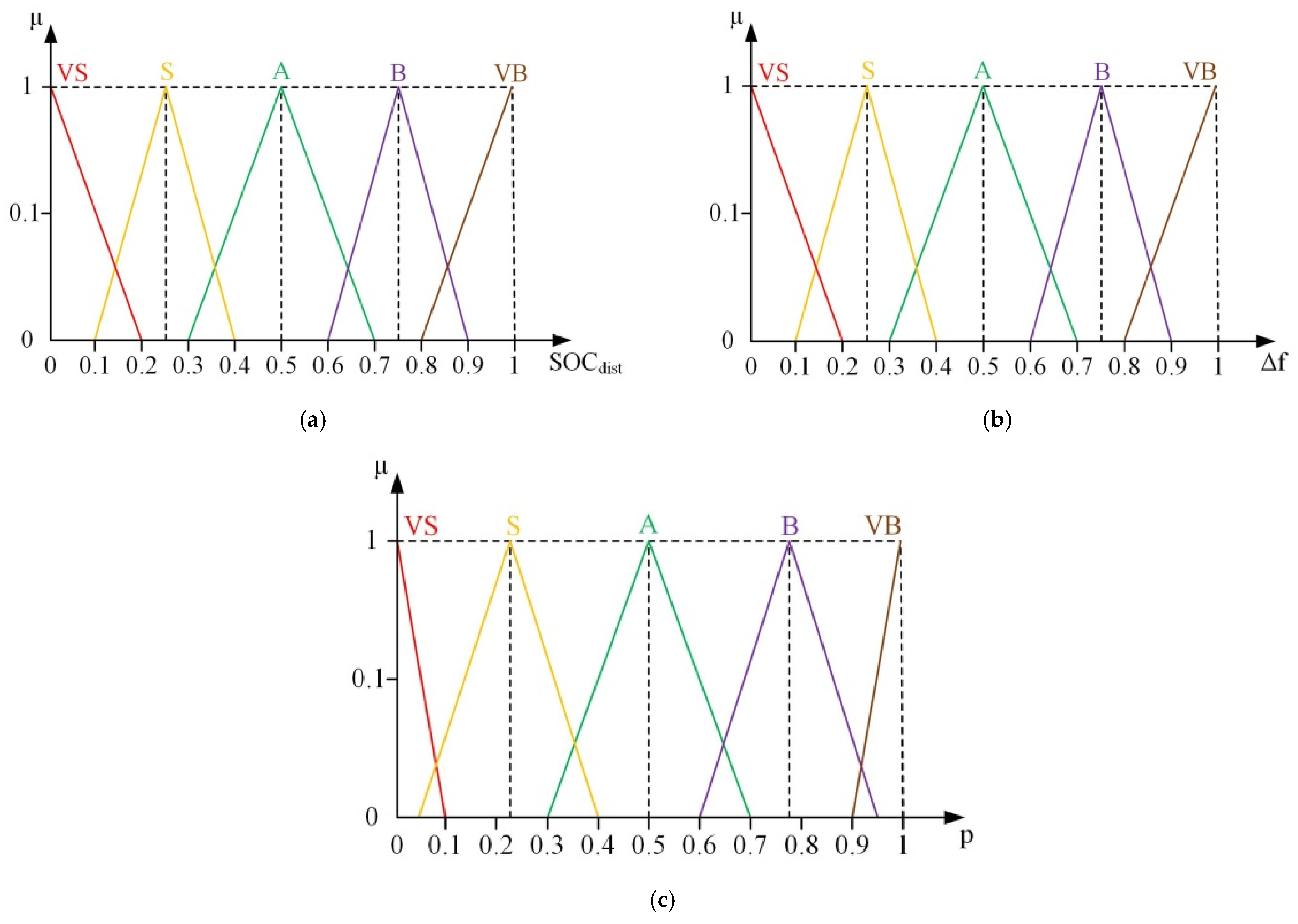
Figure 4.
Simplified diagram of system frequency control supported by the PEV aggregator.

Figure 5.
Calculated equivalent battery capacity with/without frequency support implementation.
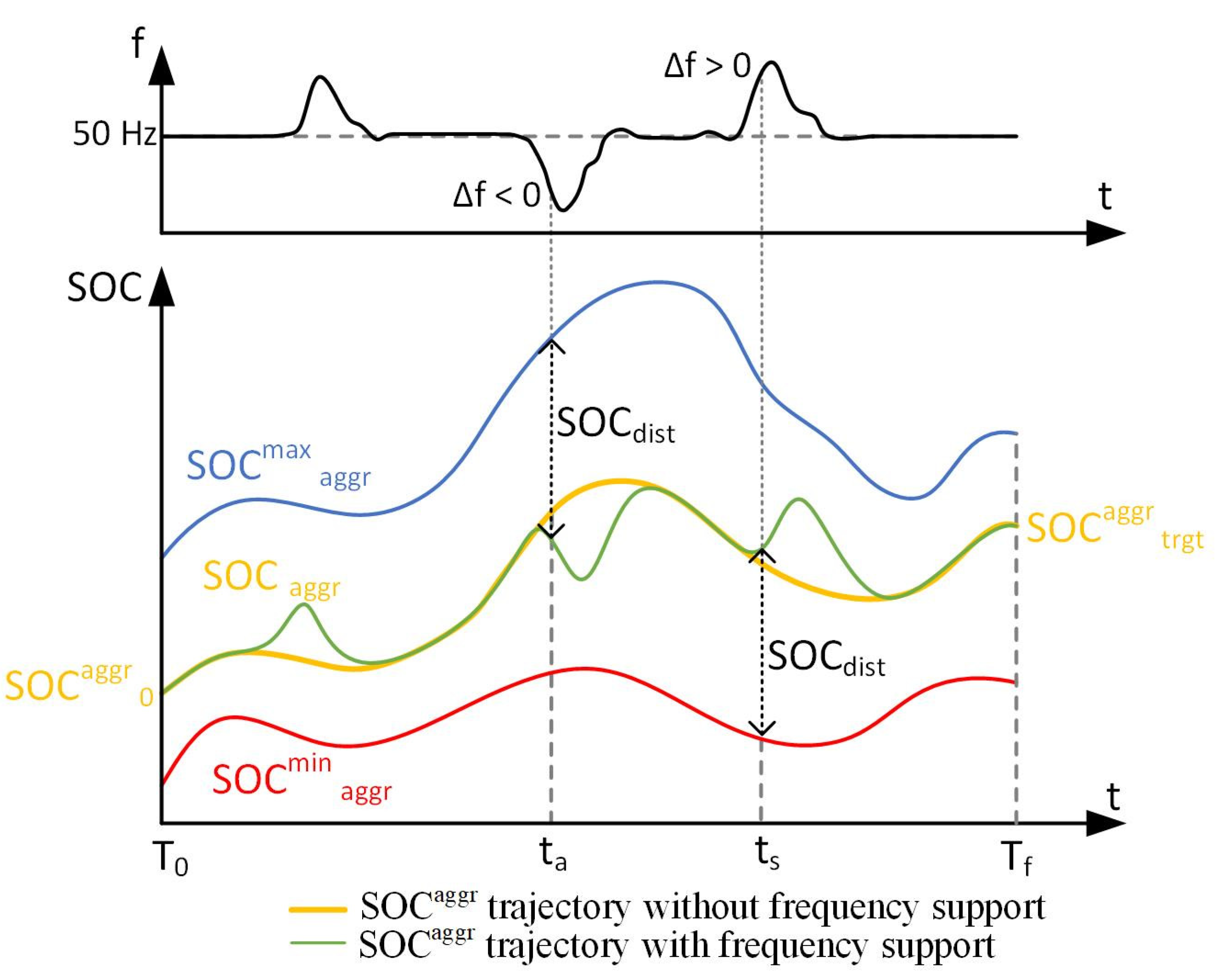
Figure 6.
A 3D graph of fuzzy system output.
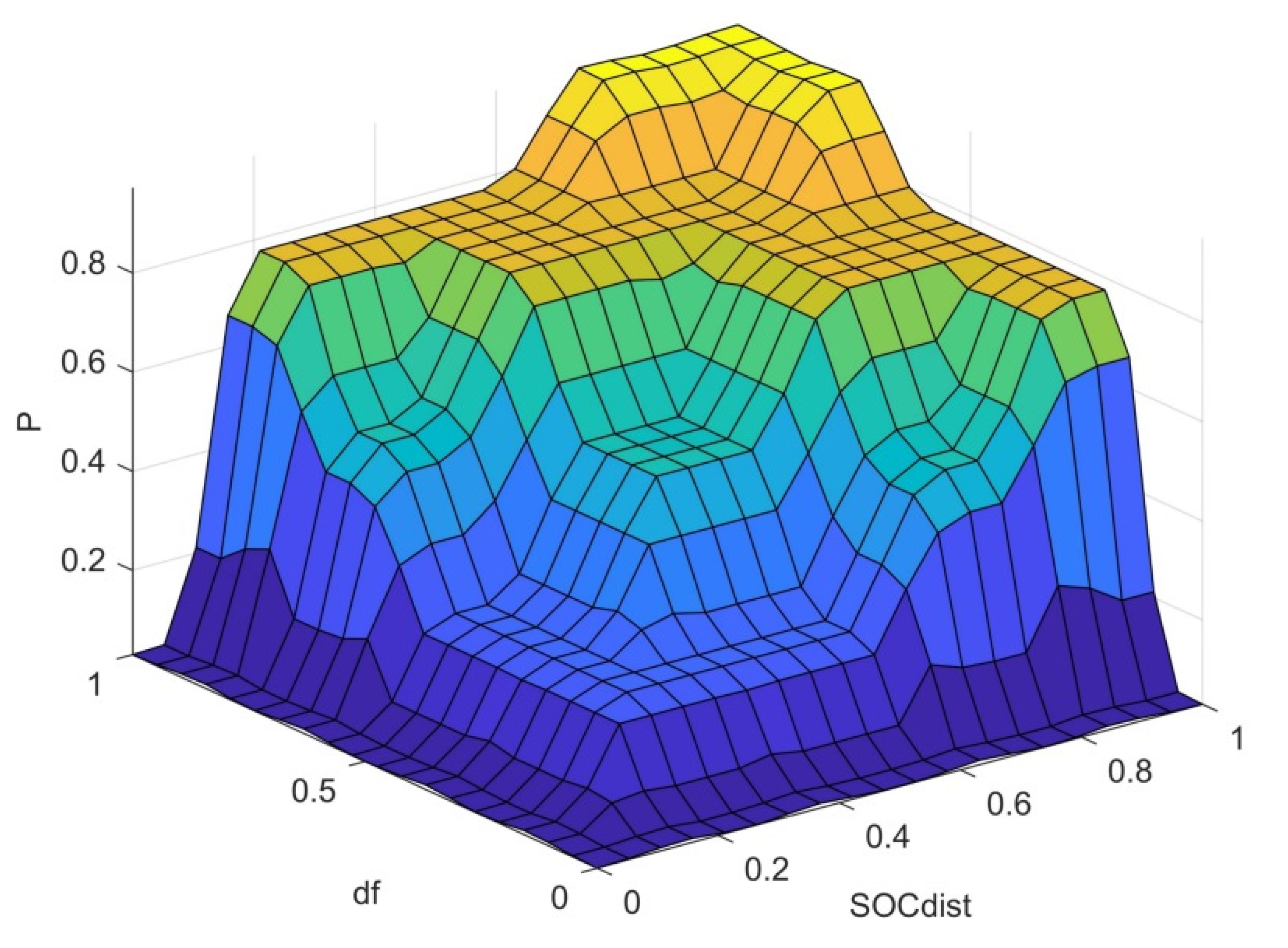
Figure 7.
Transfer function block diagram representation of an isolated system with steam, hydro, diesel, and gas power generation units with their controllers and PEV support.
Figure 7.
Transfer function block diagram representation of an isolated system with steam, hydro, diesel, and gas power generation units with their controllers and PEV support.

Figure 8.
Optimal SOC trajectories of PEVs connected to a charger.
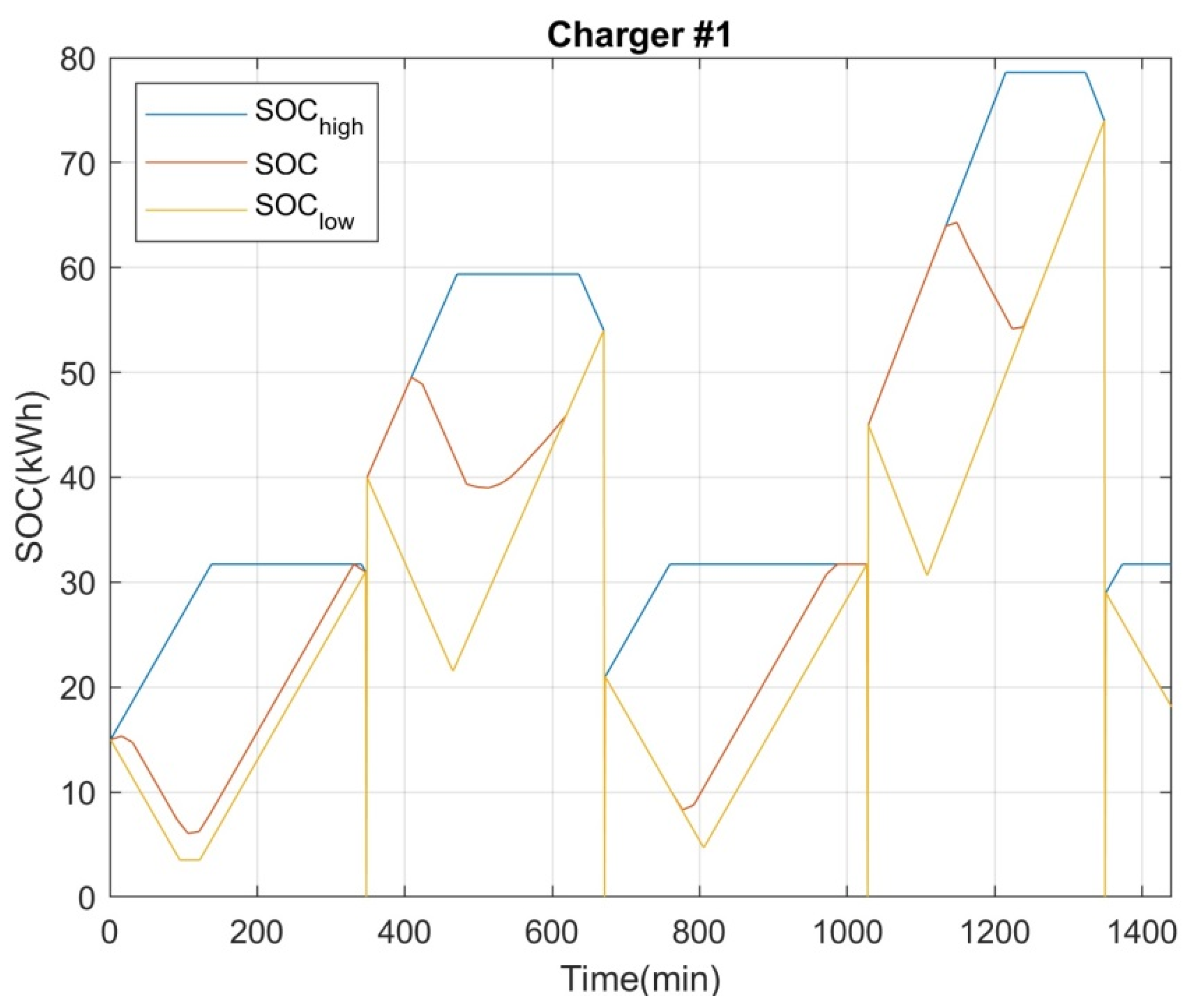
Figure 9.
(a) Capacity for every PEV battery; (b) capacity for equivalent battery.

Figure 10.
(a) A random frequency deviation from nominal value (50 Hz); (b) power generation when fuzzy frequency controller is implemented either separately or in total.
Figure 10.
(a) A random frequency deviation from nominal value (50 Hz); (b) power generation when fuzzy frequency controller is implemented either separately or in total.
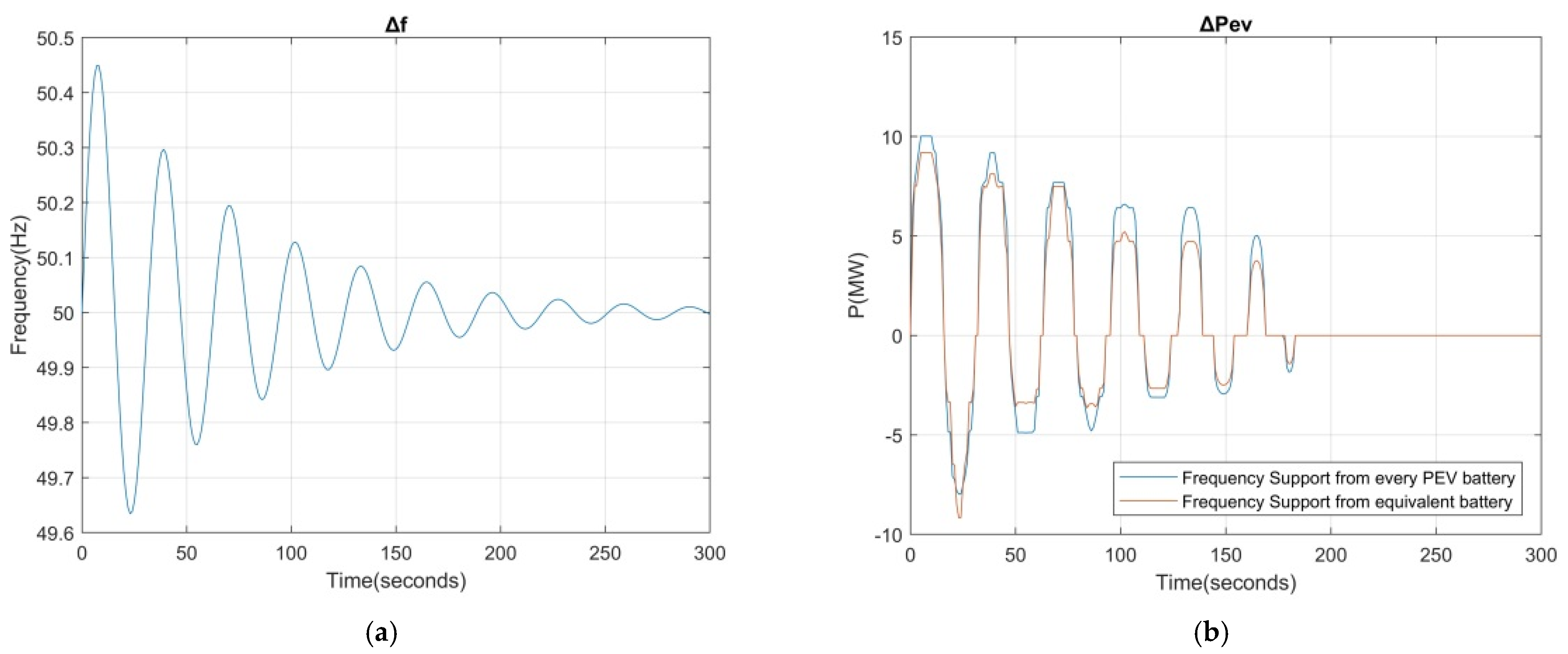
Figure 11.
Frequency support according to the number of connected vehicles.

Figure 12.
PEV power change with respect to their number (load convention).

Figure 13.
Total power generation from a certain number of PEVs with respect to load change.

Figure 14.
Total power generation from a certain number of PEVs depending on SOC level.

Figure 15.
(a) SOC restored to previous values after increasing due to power absorption; (b) SOC trajectory before/after frequency support.
Figure 15.
(a) SOC restored to previous values after increasing due to power absorption; (b) SOC trajectory before/after frequency support.


Table 1.
Fuzzy rules for power change factor estimation.
| VS | S | A | B | VB | ||
| VS | VS | VS | VS | VS | VS | |
| S | VS | S | S | M | B | |
| A | VS | S | M | B | B | |
| B | VS | M | B | B | VB | |
| VB | VS | B | B | VB | VB | |
Table 2.
PEV battery specifications.
| Price | Battery Capacity (kWh) | Nominal Power (kW) |
|---|---|---|
| Low | 35.3 | 7.3 |
| Low–medium | 51.5 | 10.25 |
| Medium | 63.9 | 9.5 |
| High–medium | 83.6 | 10.8 |
| High | 95.6 | 12.8 |
Table 3.
Generation capacity of Crete.
| Power Plant | Gas Turbine | Steam Turbine | Diesel Turbine | Installed Power (MW) |
|---|---|---|---|---|
| Heraklion | 118.47 | 105 | 49.12 | 272.59 |
| Chania | 302.69 | 42.5 | - | 345.19 |
| Lasithi | - | 100 | 102.24 | 202.24 |
| Total (MW) | 421.16 | 205 | 151.36 | 820.02 |
Table 4.
Power system parameters.
| Steam Turbine Parameters | ||
| Steam turbine governor time constant | 0.1 s | |
| Steam turbine time constant | 0.4 s | |
| Coefficient of reheat steam turbine | 0.5 | |
| Reheat time constant | 10.0 s | |
| Steam speed governor regulation parameter | 0.6 p.u. | |
| Steam turbine integral controller gain | 1 p.u. | |
| Hydraulic Turbine Parameters | ||
| Water time constant | 1 s | |
| Main servo time constant | 0.2 s | |
| Speed governor rest time | 5.0 s | |
| Transient droop time constant | 28.75 s | |
| Hydro speed governor regulation parameter | 0.25 p.u. | |
| Hydro turbine integral controller gain | 0.3 p.u. | |
| Diesel Turbine Parameters | ||
| Equivalent speed governor time constant 1 | 1.0 s | |
| Equivalent speed governor time constant 2 | 2.0 s | |
| Equivalent speed governor time constant 3 | 0.025 s | |
| Diesel turbine power generation time constant | 3.0 s | |
| Diesel turbine governor gain | 1.0 | |
| Diesel speed governor regulation parameter | 0.2 p.u. | |
| Diesel turbine integral controller gain | 0.1 p.u. | |
| Gas Turbine Parameters | ||
| Speed governor lead time constant | 0.6 s | |
| Speed governor lag time constant | 1.0 s | |
| Valve positioner constant | 1.0 | |
| Valve positioner constant | 0.05 | |
| Valve positioner constant | 1.0 | |
| Combustion reaction time delay | 0.3 s | |
| Fuel time constant | 0.23 s | |
| Compressor discharge volume time constant | 0.2 s | |
| Gas speed governor regulation parameter | 0.1 p.u. | |
| Gas turbine integral controller gain | 0.2 p.u. | |
| Power System Parameters | ||
| Power system gain | 0.06 p.u. | |
| Power system time constant | 20.0 s | |
Publisher’s Note: MDPI stays neutral with regard to jurisdictional claims in published maps and institutional affiliations. |
© 2021 by the authors. Licensee MDPI, Basel, Switzerland. This article is an open access article distributed under the terms and conditions of the Creative Commons Attribution (CC BY) license (https://creativecommons.org/licenses/by/4.0/).
Share and Cite
MDPI and ACS Style
Dakanalis, M.; Kanellos, F.D. Efficient Model for Accurate Assessment of Frequency Support by Large Populations of Plug-in Electric Vehicles. Inventions 2021, 6, 89. https://doi.org/10.3390/inventions6040089
AMA Style
Dakanalis M, Kanellos FD. Efficient Model for Accurate Assessment of Frequency Support by Large Populations of Plug-in Electric Vehicles. Inventions. 2021; 6(4):89. https://doi.org/10.3390/inventions6040089
Chicago/Turabian StyleDakanalis, Michail, and Fotios D. Kanellos. 2021. "Efficient Model for Accurate Assessment of Frequency Support by Large Populations of Plug-in Electric Vehicles" Inventions 6, no. 4: 89. https://doi.org/10.3390/inventions6040089